


Introduction
The ground-wave is the most important mode of propagation of radio waves in connection with glaciology. For the interaction between the medium and the wave the following facts are often prevalent and of special interest in cold regions:
-
(1) Propagation over non-homogeneous earth,
-
(2) Presence of stratified media,
-
(3) Low values of conductivity and dielectric constant in the upper strata.
A radio wave which propagates along the Earth's surface is, however, also influenced by atmospheric refraction. As the frequency is increased, which generally gives higher accuracy and resolution in remote sensing, this effect becomes more pronounced. At the same time the roughness of the surface must be taken into account.
The seasonal variations to be encountered are thus due to changes in the electrical and topographical properties of the ground, as well as in the propagation conditions in the atmosphere. Even if it were desirable for interpretation or comprehension to separate these various effects, it is in practice very difficult to decide what causes the observed effects. Further, in propagation over non-homogeneous and stratified earth we have to assume that the sections and layers with different electrical properties are individually homogeneous, which often is far from true.
Ground-wave propagation has been dealt with theoretically in many important papers for almost a century. It is not the purpose of this paper to review this progress, nor to give a thorough treatment of the mathematical solution of the various ground-wave problems. The intention is here to consider this type of propagation from the engineering point of view and to emphasize mainly some practical aspects of importance in remote sensing.
Model for ground-wave propagation
In most practical cases of ground-wave propagation in cold regions, the ground-wave field strength can be expressed by
where E s represents the surface wave, f(h1 and f(h2) are height-gain functions.
We begin discussing the conditions for a flat earth and then continue with the influence of the curvature of the earth. The SI system of units is used throughout the discussion and a time factor exp (jwt) is assumed.
Basic relations
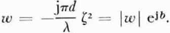
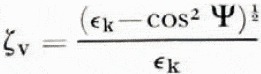
The fundamental part of the surface-wave field Es is the attenuation function A which is mathematically very complicated but reveals many interesting properties concerning the Earth's surface. The attenuation function is given in almost all text-books on radio-wave propagation, but we prefer here to show it graphically (Fig. 1) as a function of the so-called numerical distance, originally introduced by Reference SommerfeldSommerfeld (1909). The numerical distance depends in turn on the wavelength, the distance between transmitter and receiver, and the electrical properties of the ground. Slightly simplified and for vertical polarization it is given by
Here d is the distance, λ the wavelength and ζ the normalized surface impedance. (There is a similar expression for horizontal polarization, which holds for most of the formulas given throughout the paper.)
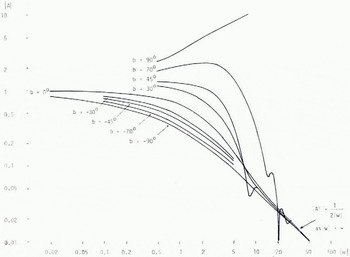
Fig. 1. Attenuation function \A\ versus numerical distance |w|. (Reference NortonNorton, 1936; Reference King and SchlakKing and Schlak, 1967.)
The surface impedance Z is defined as the ratio of the tangential electric field component to the tangential magnetic field component at the interface between air and ground for a plane wave. The properties of the ground-wave are fully determined by the surface impedance, so this is a very useful concept in studying both homogeneous and stratified surfaces.
The two phase angles, b of the numerical distance and a of the surface impedance, are very important for the. behaviour of the surface wave and will be treated seriously in the discussion to follow. They are related by the expression
For a homogeneous surface b ≤ o and the curves in Figure 1 for b-values from o down to —Π/2 are valid. Λ wave which has such an attenuation with regard to w is often called the Norton surface wave due to Reference NortonNorton (1936, 1941) who thoroughly investigated the propagation conditions for a homogeneous Earth and published numerical values of the attenuation function.
In his original work Sommerfeld (1909) touches the question whether there is a connection between the wave propagating along the Earth's surface and a guided wave. It was not until almost 50 years later that epoch-making discovery was made in this field. Several investigators studied propagation over a stratified Earth (Reference Barlow and CullenBarlow and Cullen, 1953; Reference Barlow and KarbowiakBarlow and Karbowiak, 1954; Reference WaitWait, 1953, Reference Wait1957) and threw light on this problem. Reference Wait and LangerWait (1962[b]) suggested that the total surface wave was composed of the Norton surface wave and, in addition, a trapped surface wave or Barlow wave, which occurs under special conditions for which the angle b > o, i.e. over a surface with highly inductive impedance. Such types of surfaces can exist when an ice layer is above the sea, or snow covers the ground, and are thus very interesting for propagation in cold regions. In these cases the upper curves of Figure 1 are valid.
The variations shown for these curves, especially for |w| > 5, are due to interference between the Norton surface wave and the trapped surface wave, which waves have different phase velocities (Reference King, King, Cho, Jaggard, Bruckner and HustigKing and Schlak, 1967). The discovery of the trapped surface wave enables us to explain some interesting experimental results, but at the same time this remarkable behaviour of |A| for b > o is a complicating factor in interpreting results in general. We shall come back to this later.
For large values of |w| when b is negative, it is seen that A varies as (2|w|)-1. This is also true for not too large positive values of b. These facts are evident from a series expansion of the attenuation function (Wait, 1962[b]):
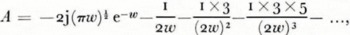
the whole of which is valid for |w| ≫ 1 and o <b < 2π. The first term of Equation (5) represents the trapped surface wave, and for the case — 2π < b < o the same expression, Equation (5), applies, except for this first term. The rest of the series corresponds to the Norton surface wave.
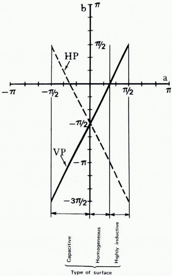
Fig. 2. Schematic classification of surface by the phase angles a and b. VP denotes vertical and HP horizontal polarization.
It is thus true that the nature of the attenuation function depends on the sign of the angle b. For historical reasons, principally this angle has been dealt with in the earlier literature as the surface impedance concept has been commonly used only in recent years. It might, however, be more useful to consider the angle a. It characterizes the properties of the surface more directly while b more or less describes the effect of the polarization of the wave. As can be seen from Figure 2, each type of surface lies within a certain interval of a which is the same for both polarizations. On the other hand the angle b is different for vertical and horizontal polarization.
The amplitude of the attenuation function has been discussed here. It should be mentioned that similar effects do occur for the phase of A.
For a homogeneous surface the normalized surface impedance is
at vertical polarization and
at horizontal polarization, where
€ is the relative dielectric permittivity, σ the conductivity and Ψ the grazing angle. The phase angles a are then, if we assume grazing incidence,
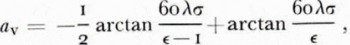
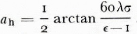
For a perfect dielectric a v = o, while a v = π/4 corresponds to a perfect conductor.
The transition from a homogeneous to a horizontally stratified Earth can be accomplished by multiplying ζ by a correction factor which accounts for the influence of the substrata. Wait (1962[b]) defines this factor
where Z 1 is the surface impedance of the first layer and K1 its intrinsic impedance. Z1, depends on the thickness of the upper layer and on the electrical parameters of the upper and lower layers. An analysis of Q for a two-layer surface shows that if the upper layer is electrically thin and if there is an abrupt change of the intrinsic impedance at the interface, the angle b assumes positive values, which is not possible in the case of a homogeneous surface. (Wait, 1962[b]). The limiting case when b = π/2 is obtained for a surface where the upper medium is a thin dielectric layer and the lower medium is a perfect conductor.
Due to seasonal variations of the electrical properties, the sign of the angle b can thus change, e.g. when the sea is covered with ice.
Attention should be drawn here to the fact that a corrugated surface may also exhibit inductive properties, provided that the irregularities are small compared with the free-space wavelength. This might cause some trouble in measuring the electrical parameters of layered structures.
Simplified ground-wave formula
We have now discussed some of the fundamental properlies of the attenuation function, which is included in Equation (I) for the ground-wave field strength. The next step is to find a formula suitable for the calculation of the field strength.
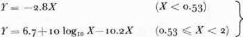
If the effect of the ground conductivity is neglected, Equation (i) can be written in a very simple way (Reference Blomquist, Désirant and MichielsBlomquist, 1960). Such a limitation is amply accurate in non-fertile areas at frequencies above 30 MHz. The conductivity values in Arctic regions are often found to be as low as 10-5 S/m. If we use the propagation factor Ff , which is the actual field strength relative to its value in free space, the flat-Earth formula can be expressed (in dB)
where
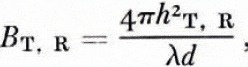
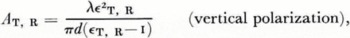
hT and hR are the antenna heights, d the distance, λ the wavelength, and ɛT and ɛR the relative dielectric permittivities. The flat-Earth formula is valid well below the first lobe maximum for distances d < 12 × 103 λ ⅓ with an error of less than 1.5 dB at the distance limit.
The restriction above to low conductivity areas is not too serious. Higher conductivity values could be accounted for by introducing a correction, which enables us to extend the use of Equation (10) even to sea-water (private communication in 1974 from L. Ladell).
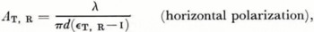
If the ratio h/λ is large, the B-terms in Equation (10) are dominant, which means that the surface wave, represented by the A-terms, has no importance, and we gain no information on the ground properties. We find that F degenerates to the well-known approximate formula
This height is about hλ= 5 for propagation over water. Above this height there is no difference between the fields for vertical and horizontal polarization, and Equation (13) is thus applicable for both polarizations, but, in fact, we are no longer dealing with the actual ground-wave.
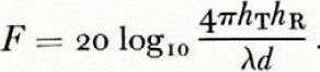
It is very complicated to make a strictly mathematical treatment of the influence of the Earth's curvature. Equation (10) can be extended, however, up to distances where the diffraction field becomes predominant by applying a curvature correction using only simple mathematical expressions (Reference BlomquistBlomquist, 1973). The correction is a function of a normalized distance X
where a is the Earth radius and k the Earth radius factor, which is 4/3 for the standard radio atmosphere. The effect of the troposphere is thus taken into account in the curvature correction, assuming a tropospheric model where the refractive index decreases linearly with increasing height. This is practically true for the lower part of the troposphere.
The curvature correction in dB to be applied to the flat-Earth formula is
It has, however, been found that (he correction can be used for distances up lo X = 4.5 with an error less than 1.5 dB. X = 4.5 corresponds to d = 219 km at λ = 10 m and d = 102 km at λ = 1 m, both for k = 4/3. For distances X > 4.5 the effect of tropospheric scatter must be considered. The correction in Equation (15) can easily be computed by means of a nomogram or a slide-rule. Thus the smooth spherical-Earth propagation factor can simply be written
G. Millington (private communication in 1974) has suggested a similar procedure concerning the effect of the curvature. His method is based on the flat-Earth formula for d<10λ1 and the diffraction curve for d > 4o λ1 which is calculated by using one term only. For the transition region the field is represented as a cubic expansion of a distance variable.
The problem of propagation over non-homogeneous Earth is of great complexity. Analytical studies of such propagation phenomena have been conducted for many years. Of great importance here are mixed paths including sea ice, sea-water, and snow-covered land. As regards the problem of calculating the field strength, Reference MillingtonMillington (1949) has given an excellent semi-empirical solution, which is accurate enough and very suitable for practical use. The method assumes that field-strength curves are available or can be calculated for the different sections of the path, which are assumed to be individually homogeneous. Equation (10) includes the Millington method for a path consisting of two sections. The subscripts T and R denote the terminals of a path, which might be over ground with different dielectric constants. However, the formula given is not valid in the vicinity of the boundary separating the two sections.
In the case of diffraction by obstacles, Equation {16) for a smooth spherical Earth must be supplemented by an obstacle correction. We shall use here the diffraction model due to Epstein and Peterson (1953). This model is chosen for its simplicity and accuracy over very rough terrain. In it the overall propagation factor Fur (in dB) is calculated as the sum of the Fresnel—Kirchhoff diffraction propagation factors for each of the main obstacles along the path.
We have now considered the two limiting propagation eases where the spherical Earth can be regarded as smooth and where it can be represented by a number of knife edges. For a given terrain profile these two cases indicate the low- and high-frequency ends respectively of the range concerned. To solve the problem of finding a model valid for the whole frequency range we have to specify a bridge function or a weighting factor in terms of the propagation factors of these two extreme cases.
An empirical propagation model, denoted F R, will be introduced, which is based on the smooth spherical-Earth field F B and the obstacle diffraction field F E (Reference Blomquist and GudmandsenBlomquist and Ladell, 1975). These two propagation factors are easy to calculate quite accurately and do not need complicated computer technique.
The model F R is the negative square root of the sum of the squares of F B and F EP, expressed in dB,
This square-root field is always less than either of the calculated two components, as is seen in Figure 3. This model has a low-frequency asymptotic value of the propagation factor equal to F B and a high-frequency asymptotic value equal to FEP, which is in accordance with the assumption.
A very difficult case of stratified Earth to treat appears when the upper layer thickness varies along the path. Reference BaharBahar (1972) has considered this problem fundamentally. Though reciprocity is valid between the transmitting and receiving terminals over such a path, the surface impedance might not be the same for both directions of propagation. It is, however, not so easy to test by experiments the validity of such theoretical predictions.
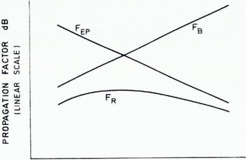
Fig. 3. Sketch of frequency dependence for some propagation models.
Determination of the electrical characteristics of the earth's surface
The ground constants, the dielectric permittivity, and the conductivity, are all but constant at any one time. They vary markedly from time to time due to changes in the surface conditions. Measurements of the electrical parameters may thus provide a means by which interesting information on glaciological media can be achieved.
There are two main methods using the ground-wave for the determination of the ground constants: the ground-wave attenuation method and the wave-till method. Both are based on the properties of the attenuation function discussed earlier, and—contrary to direct measurements on samples, the results of which often are inconclusive as the natural state of the samples has changed—these radio-wave methods give the effective values as weighted averages over a volume of Earth, the size of which depends on the frequency and the penetration depth.
Measurements of the ground-wave attenuation
Measurement of the attenuation with distance along a path makes it possible to deduce the electrical constants by comparison of the results with propagation curves prepared for various sets of the two constants. An advantage of this method is that measurements can be performed continuously for long periods of time over a certain path, or can be made from a moving vehicle or aircraft thus covering large areas. The method has been used for mapping the conductivity by means of LF-waves (Broms, 1970).
The ground-wave method is often said to be unsuitable for detailed measurements of the ground constants over given small areas. This is not quite true. If the frequency is properly chosen this can be accomplished at least for the dielectric permittivity as will be shown later. Λ similar procedure is the measurement of the change of phase with distance. This method has been found to be a more sensitive means of locating discontinuities in the ground than that provided by measurement of attenuation.
Wave-tilt method
This is an in situ method rather than a tool to be used in remote sensing technique, but most of the measurements which have shown variations in the electrical constants, have been carried out by this method (Reference KingKing, 1968; Reference Blomquist, Koch and LjungbergBlomquist, 1961, 1970; Reference McNeill and HoekstraMcNeill and Hoekstra, 1973). The method is based on the fact that the electric field received from a vertically polarized transmitting antenna after propagating along the surface of the Earth also has a horizontal component in the direction of propagation. Thus the field vector is lilted forward.
In general the vertical and horizontal components of the field are out of phase, thus forming an elliptically rotating vector in the plane of propagation. The angle between the major axis of this ellipse and the vertical axis is called the angle of tilt. In the literature the radio wave is often said to be elliptically polarized in this case, but this is improper as, according to the definition, an elliptically polarized wave has the rotating field vector in the plane perpendicular to the direction of propagation. The ground constants are determined by the axial ratio and forward tilt of this ellipse. By means of a rotatable antenna and suitable data acquisition it is possible to study in detail the variation of the electrical constants during different weather conditions.
Size of the “effective volume”
Ground-wave measurements produce values which are averages of the electrical parameters over an “effective volume”. The size of this volume depends on the frequency and also the type of method used. The extent to which sub-strata influence the effective value of the ground constants depends on the pentration depth, while it is more difficult to determine the area along the path over which the measurements are sensitive.
VHF-measurements by means of the wave-till method have indicated that the value obtained is typical of a surface area having the shape of an ellipse, (he major axis of which is coincident with the line joining transmitter and receiver. The receiving antenna is assumed to be at the focus farthest from the transmitter. The sensitive area is thus particularly at the site of the receiving antenna and somewhat—roughly the wavelength times the dielectric constant—in the direction of the transmitter (Blomquist, 1960).
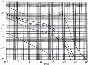
Fig. 4. Penetration depth as a function of frequency. (a) Very dry ground, (b) Fresh water, (c) Average ground, (d) Wet ground.(e) Sea-water.
Using the ground-wave method, account is also taken of the corresponding conditions at the transmitter site. As the wavelength is increased, these two areas surrounding the antennas are thus enlarged and will finally be joined together forming the first Fresnel zone.
The depth of penetration is commonly defined as the depth at which the wave has been attenuated to e-1, i.e. 37% of its value at the surface of the Earth. It depends on the ground constants and the frequency as is illustrated by the examples in Figure 4. The influence is, however, decreasing exponentially with depth, which means that the radio wave is most sensitive to the upper strata.
So by proper choice of the frequency it is possible to obtain results which are averages over either a small area or a large area of the surface of the Earth. For the VHF-region the following expressions can be used as a rough estimate of the size of the ellipse surrounding the antenna (Blomquist, 1960): major axis = λ (+8ɛ5) and minor axis = 4.47ɛ ½ ɛ. Assuming average ground with ɛ = 15 this yields 20λ and 17.3λ, respectively, and the area of the ellipse = 272 λ2.
Thus, the use of very short wavelengths enables us to study the properties of rather small areas. Considering the dependence on height of the ground-wave, which was discussed in connection with Equation (10), the increasing area resolution is, on the other hand, restricted downwards as the value of h\λ must be comparatively small in practice.
Some experimental results
Most of the results reported on ground-wave measurements are not relevant to cold regions, nor do they exhibit seasonal effects. We have therefore only a limited number of experiments (hat can reflect the variations expected from the foregoing analysis of the attenuation function.
Figure 5 shows a comparison between measured and calculated propagation factors as a function of distance for vertical polarization at 40 MHz in slightly irregular terrain. The transmitter sites were located at distances from 5 to 24 km from the receiver, the antenna height of which was 24 m. The antenna height of the transmitter was as low as 1 m. Thus pertinent information is gained mainly on the Earth conditions in the vicinity of the transmitting antenna. The propagation factor is calculated by the FB -model, Equation (16), for three values of the Earth-radius factor k = I, k = 4/3, and k = ∞. The measurements were made in northern Sweden during winter, so the meteorological conditions are likely to be represented by a value of k < 4/3, which is in fair agreement with the measured values. During the measurements, the variations of the relative dielectric permittivity were also separately studied by the wave-tilt method. It was found to vary between 5 and 9 during the period concerned. A value ɛ = 7 has been used in the calculations of FB These measurements give a very good idea of the overall conditions along the path and are very useful for the concept of transmission loss for example.
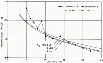
Fig. 5. Comparison between calculated and measured field during a winter period as a function of distance at 40 MHz in slightly irregular terrain.
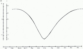
Fig. 6. Average annual variation of dielectric permittivity and field strength at 50 MHz and low vertically polarized antennas.
If we now continue this type of measurements for a long period of time, we obtain information on how the ground properties vary with the season. The curve in Figure 6 shows the annual variation of the ground-wave field strength at 50 MHz, vertical polarization, in central Sweden. This curve is the average over a period often years. The corresponding value of the dielectric constant e has been determined by means of the. FB-model, Equation (16). The rapid changes of ɛ in spring and autumn are mainly due to variations in the moisture content of the upper surface layers. During a rainy summer the, minimum of the curve is of course not so strongly marked.
The situation in winter has been represented by a dashed curve as it is very complicated and needs further discussion. The values of € for snow and ice are very low, which in general reduces the resulting effective dielectric constant for the volume over which averaging occurs. ( Compare the example given in Figure 5.) This would indicate another minimum value in winter for the annual dependence of ɛ in Figure 6. Under special conditions of stratified Earth, which commonly occur in winter, the behaviour of the winter part of the curve in Figure 6 might, however, be quite different. This is apparent from Figure 7, which is based on long-term measurements at 44 MHz vertical polarization over a very short path. The depth of snow in winter was less than 20 cm, but its state changed due to temperature variations both below and above the freezing-point. The measured field strengths have been hopefully arranged in groups with regard to the moisture content.
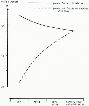
Fig. 7. Average influence of mosure content on ground-wave field strength for frozen and unfrozen ground. 4.4 MHz, vertical polarization.
When the ground was not frozen or covered with snow, the field strength varied in accordance with the solid part of the curve in Figure 6. But for the winter case the result is rather surprising. Having checked the combination of wavelength and distance to the transmitter, we have found that this result might be explained by the high values of the attenuation function which can occur when b > o (Fig. 1).
More-or-less frozen snow-covered ground might guide the radio-wave in a way similar to that in tropospheric duct propagation. So even if the result observed is not a conclusive proof of the existence of a trapped surface wave, it is a clear indication that a wave of the type foreseen by Wait may occur in winter.
It has been stated before that the upper strata are the most important part of the “effective volume”'. This is shown in Figure 8, which gives the correlation between the field strength of the ground-wave and the temperature at different depths of the ground. These measurements are from a period of one year, with the air-temperature varying between — 15°C and + 30° C. The temperature at the depth of 50 cm showed a variation of 17 deg. It is seen that the correlation is very good close to the surface. The influence of temperature on field strength is, however, probably indirect. In fact, moisture content is the major factor, but variation in it is often related to temperature variation.
An example of measurement of the dielectric constant by the wave-tilt method is given in Figure 9, where the conditions at a boundary between clay soil and an asphalt road have been studied at 44 MHz (Blomquist, 1961). The measured values of angle of tilt Θ are indicated by points. The sudden change in the ground properties gives a jump in the Θ curve. Near the boundary the value of Θ is determined by the value of each medium is a complicated way. The fluctuations in the curve for the asphalt road are probably due to inhomogeneities in the layer below the asphalt. This is an example where detailed measurements have been performed over a small area. An effect similar to that in Figure 9 would have occurred if there had been ice instead of the asphalt layer.
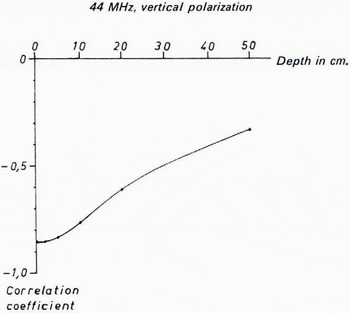
Fig. 8. Correlation between field strength and temperature at various depths in the ground.
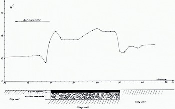
Fig. 9. Measurements of the angle of tilt Θ at a boundary between sections of clay soil and an asphalt road.
Reference Hoekstra, Hoekstra, Delaney, Sellman and InceHoekstra and others (1975) have made measurements of the surface impedance in the range from VLF up to about 700 kHz in the North American Arctic. They have shown that extreme local detail in the Earth geology can be mapped by ground-waves. An example of their study is given in Figure 10. Compare their result with the behaviour of the angle of tilt in Figure 9.
Reference BiggsBiggs (1971) has studied propagation over mixed paths for the HF-range in the Arctic Ocean. He found that the Millington method was valid even if stratified media were involved in mixed paths and that the propagation irregularities obtained over such paths provide a mechanism for identification of sea-ice boundaries.
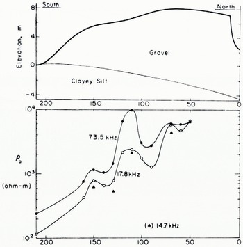
Fig. 10. The geological cross-section and the apparent resistivity measurement on the ground at several frequencies (Hoekstra and others, 1975).
Another way of studying ground-wave propagation is to simulate experiments using modelling techniques. This might be an inexpensive but sometimes also a problematic way of confirming existing theories. In quite a recent paper King and others {1974) have successfully investigated ground-wave propagation over cylindrical homogeneous paths and two-section mixed paths by the use of microwave models. As exemplified in Figure 11 they found a good agreement between calculated and measured values for propagation over two-section mixed paths consisting of “Plexiglas” (polymethylmethacrylate) and water and metal. A frequency of 4.765 GHz was used.
Effect of depolarization
In treating propagation over the surface of the Earth, the depolarization effect must not be overlooked. This effect might overshadow the influence of the variations of the electrical parameters, but polarization discrimination might also provide useful information on the ground properties and aid in understanding of their relationship with various remote-sensing signatures.
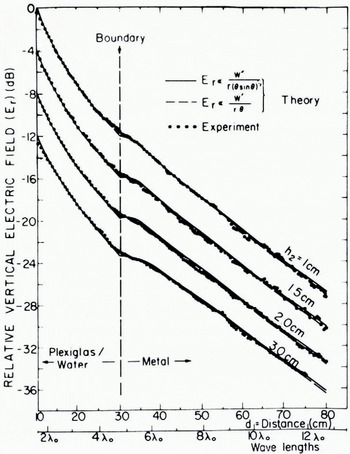
Fig. 11. Dipole excited ground-wave field versus distance d over two-section cylindrical {experimental) and spherical (theory) mixed paths composed of “Plexiglas” (polymethylmethacrylate) over water and metal. Frequency = 4.765 GHz, boundary at di = 30 cm, h1- 1.5 cm, and a = 125 cm (King and others, 1974).
Scattering and absorption are the two main mechanisms causing depolarization of ground-waves. Figure 12 gives the variability with location of the depolarization factor as a function of frequency for measurements made in various types of terrain with low antennas (less than 10 m) (Reference BlomquistBlomquist, 1965). The depolarization factor is here defined as the ratio of the orthogonally polarized field component to the originally polarized component. It should be noticed that for high frequencies and small percentages of locations, the orthogonal component is larger than the transmitted. There is also a variability in time. In a forest, the field is often set up by direct and scattered waves. When the trees move in the wind, a depolarization fading phenomenon occurs, which amounts to several decibels in amplitude at quite moderate wind velocities. On the other hand, there is a slow variation due to the fact that the electrical properties of the ground vary with the season. In interpreting ground-wave field measurements, these rather complicating depolarization phenomena must be kept in mind.
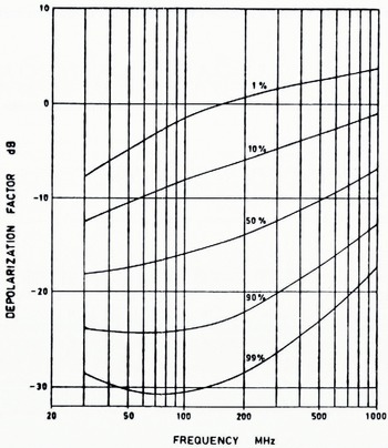
Fig. 12. Depolarization factor not exceeded for given percentages of locations.
On further investigations of the ground-wave
In the previous discussion we have found that the use of ground-wave propagation phenomena might be helpful for several diagnostic purposes. We have also pointed out some cases where problems may arise.
One unfavourable condition, probably the most important, is due to the composite effect of terrain and atmospheric influences on wave propagation. This makes it difficult to treat separately the various effects that contribute to the resulting field. To what degree the ground-wave propagation is affected by other properties than those of the Earth differs from time to time and is more or less easy to determine. As an example of one extreme it might be observed that the field strength over a path is considerably increased for a small percentage of the time. On such occasions the field is probably governed by tropospheric layer propagation mechanisms and not by ground-wave propagation along the path. The occurrence of such phenomena varies with the season without the occurrence of any seasonal effect of the ground-wave.
To facilitate the interpretation in other less evident cases, it might be worth-while to analyse the main characteristics of the wave, i.e. the amplitude, the phase, the wavelength, and the polarization. It is possible but not proved that these characteristics are not all simultaneously coupled together. It has been shown that vertical and horizontal polarization may display different properties of the medium. The phase of the wave has only been mentioned in passing. This must not be interpreted as implying that a study of it would be unimportant, but it is significant that very little attention has been paid to phase studies in the literature. It is clear that a wave propagating along the Earth's surface suffers phase distortion, which in turn may reveal interesting information on the interaction between the wave and the ground, e.g. when a wave crosses boundaries between sections with different electrical properties.
A further study of the relationship between these different characteristics of the wave and their possible independence of each other is needed lo extend the possibilities of using ground-waves in electromagnetic probing applications. An interesting approach in this direction has been given by Wait (1962[a] and in several later papers). He has suggested that the resulting distortion of pulsed signals be utilized as a diagnostic tool. He has also consequently studied the propagation mechanism for transient conditions considering some idealized situations. Among Others, Reference Sivaprasad and StotzSivaprasad and Stotz (1973) have treated layered media theoretically. They have determined the reflection of a normally incident pulse from a three-layered medium, and their calculations indicate that the method may be useful in the detection of the thickness of ice layers. There seems, however, to be no experimental work which confirms these theoretical conclusions. Scattering from the roughness or irregularity of the sub-surface is likely to distort the pulse. So additional investigations are required before it is possible to decide whether the pulse response of the ground-wave can be used for probing purposes.
It should be observed here that pulse distortion may also occur due to the influence of the terrain. Multi-path effects may be a limiting factor in many practical cases, especially in irregular terrain. Propagation over non-uniform layered ground has also to be studied more thoroughly in the future. Experimental verification of the various theories is insufficient. And, conversely, the theoretical models used do not take proper account of the real features and properties of the ground.
Modelling techniques might be interesting for future investigations. In view of their apparent success in explaining some phenomena, it is, however, easy to neglect the difficulties in obtaining meaningful laboratory measurements. One principal problem is how to simulate temporal changes in the refractive index, for example. In this connection it should be mentioned that the use of minicomputers might be very helpful in future attempts to improve models and to explain experimental results.
In addition to propagation formulas it is often useful to have curves. The most comprehensive curves on ground-wave propagation are published by the C.C.I.R. (Comité Consultatif International des Radiocommunications); they include frequencies from 10 kHz up to 10 GHz except for a gap between 10 MHz and 30 MHz. The atlas of curves for frequencies above 30 MHz, is, however, out-of-print and unobtainable. The C.C.I.R. intends to prepare new curves in the near future, when the existing frequency gap will also be filled in. As regards the curves below 10 MHz, the C.C.I.R. has recently, as a temporary measure pending the new curves, added some new curves for very low conductivities (Comité Consultatif International des Radiocommunications (C.C.I.R.), 1974). This was to meet a specific need from people dealing with propagation in cold regions.
Concluding remarks
The main objectives have been to present the current state of knowledge concerning theory and experimental results on ground-wave propagation bearing on matters of glaciological interest. Although the propagation of the ground-wave has been dealt with for almost a century, some of the most valuable information of major importance in cold regions has been achieved during recent years. The new theoretical work on propagation over stratified Earth offers an explanation of the variations of the ground-wave field which have been observed, as well as implying new methods to be tested as possible aids in solving glaciological problems.
The possibility of using characteristic effects of the ground-wave as a diagnostic tool is, however, limited due to the fact that it is sometimes difficult to separate the composite effects of various propagation mechanisms which contribute to the resulting field. Further investigations of the mutual independence of the fundamental characteristics of the radio wave might overcome such difficulties.
Though excellent work has been performed for years, much research remains to be carried out before a full understanding is obtained of the complicated mechanisms connected with the interaction between the wave and the surface of the Earth, so an attempt has been made to suggest some additional investigations as suitable.
Discussion
R. T. LOWRY: You mentioned that ice looked like dry ground; what types of ice were you referring to, first-year sea ice or fresh-water ice?
A. BLOMQUIST: When I referred to a set of curves showing the penetration depth for various types of ground I said that the curve for very dry ground corresponds quite well to the situation for ice. That curve has been calculated assuming frequency-dependent values of the ground constants, which are about ɛ = 3 and σ = 10-4 S/m at 50 MHz, for example. Average ice has similar values.
W. F. WEEKS: Dr Hoekstra of CRREL has attempted to use VLF wave-tilt methods to measure the thickness of sea ice. However he has encountered severe difficulties because of pronounced lateral variations in the electrical properties of what would on the surface appear to be laterally homogeneous ice. Have you any experience in these problems and, if so, would you care to comment on them?
BLOMQUIST: I have used the wave-tilt method to study the electrical properties mainly of lake ice and in the VHF region. At these frequencies the volume over which averaging of the electrical parameters occurs is quite small compared with the situation in the VLF band, which reduces the possibility of including unexpected variations. As I have no experience myself of VLF measurements, I can only guess that varying salinity and also varying thickness of the ice layer might have contributed to the difficulties you mentioned.


