


1. Introduction
The use of acoustics to investigate snow is complicated by the fact that sometimes lower wave velocities can be observed with increasing density of snow (Reference OuraOura, 1952). This observation is at odds with elastic or viscoelastic wave propagation theory, for which higher velocities are expected for the considerably higher bulk and shear moduli of denser snow. Yet the observed wave velocities can be explained with wave propagation theory for porous materials, where a second compressional wave, also known as the ‘slow’ wave, is predicted (Reference JohnsonJohnson, 1982; Reference SmeuldersSmeulders, 2005). Even though the word ‘slow’ suggests that it is the velocity of the wave that leads to its name it can actually be shown that ‘the fast wave travels in the skeleton and the slow wave in the fluid’ (Reference CarcioneCarcione, 2007, p. 275).
Acoustic waves have been used in snow for a variety of applications. Reference OuraOura (1952), Reference SmithSmith (1969) and Reference Yamada, Hasemi, Izumi and SatoYamada and others (1974) measured acoustic wave velocities and attenuation in field and laboratory environments. Reference GublerGubler (1977) measured acceleration in the snowpack and air pressure above the snowpack for explosives used in avalanche mitigation operations. Reference JohnsonJohnson (1982) successfully used Biot’s model for wave propagation in porous materials to predict wave velocities in snow. Reference Sommerfeld and GublerSommerfeld and Gubler (1983) observed increased acoustic emissions from unstable snowpacks compared to acoustic emissions of stable snowpacks. Reference MellorMellor (1975) and Reference Shapiro, Johnson, Sturm and BlaisdellShapiro and others (1997) published extensive reviews on snow mechanics including acoustic wave propagation and proposed wave velocity as a potential index property for snow. Amongst others, Reference BuserBuser (1986), Reference Attenborough and BuserAttenborough and Buser (1988), Reference Marco, Buser and VillemainMarco and others (1996, Reference Marco, Buser, Villemain, Touvier and Revol1998) and Reference Maysenhölder, Heggli, Zhou, Zhang, Frei and SchneebeliMaysenhölder and others (2012) investigated acoustic impedance and attenuation of snow based on the so-called ‘rigid-frame’ model (Reference TerzaghiTerzaghi, 1923; Reference Zwikker and KostenZwikker and Kosten, 1947) in which the wave traveling in the pore space is completely decoupled from the wave traveling in the frame of the porous material. Recently, acoustic methods have been used to monitor and spatially locate avalanches (Reference Surinach, Sabot, Furdada and VilaplanaSurinach and others, 2000; Reference Van Herwijnen and SchweizerVan Herwijnen and Schweizer, 2011; Reference LacroixLacroix and others, 2012), to estimate the height and sound absorption of snow covering ground (Reference AlbertAlbert, 2001; Reference Albert, Decato and PerronAlbert and others, 2009, Reference Albert, Taherzadeh, Attenborough, Boulanger and Decato2013) and to estimate the snow water equivalent of dry snowpacks (Reference Kinar and PomeroyKinar and Pomeroy, 2009). Reference Kapil, Datt, Kumar, Singh, Kumar and SatyawaliKapil and others (2014) used metallic waveguides to measure acoustic emissions from deforming snowpacks. The advantage of the rigid-frame model over Biot’s model is that it is relatively straightforward to extract tortuosity of the pore space and pore fluid properties from the phase velocities of the slow wave. Applications are widespread and range from non-destructive testing, medical applications and soil characterization to sound absorption (Reference Fellah, Chapelon, Berger, Lauriks and DepollierFellah and others, 2004; Reference Jocker and SmeuldersJocker and Smeulders, 2009; Reference Attenborough, Bashir and TaherzadehAttenborough and others, 2013; Reference Shin, Taherzadeh, Attenborough, Whalley and WattsShin and others, 2013).
The rigid-frame model can be deduced from Biot’s (1956a, 1962) theory under the assumption that the stiffness of the porous frame is considerably higher than the stiffness of the pore fluid. The rigid-frame model does not account for the interaction between the pore fluid and the porous frame as does Biot’s theory. The viscous effects of the pore fluid are approximated with complex moduli in the rigid-frame model. Consequently the rigid-frame model is a phenomenological model. Biot’s model, where the viscous friction of the fluid moving relative to the solid frame is causing the observed attenuation, is a physical model instead. Under exclusion of phenomenological attenuation (e.g. complex bulk and shear moduli) the rigid-frame model is not frequency-dependent while Biot’s model, due to its explicit treatment of relative fluid motion, is. Especially in light snow and in wet snow, where the frame and the stiffness of the pore fluid are of a comparable order of magnitude, Biot theory is expected to provide better results than the rigid-frame model (Reference Hoffman, Nelson, Holland and MillerHoffman and others, 2012). Also a physical model is to be preferred over a phenomenological model as the results can be compared to complementary measurements and consequently have more predictive power. However, a disadvantage of the application of Biot’s model is the large number of properties that have to be known to solve the differential equations.
While phase velocities obtained with plane wave solutions for Biot’s theory tend to correspond relatively well with its measured counterparts, generally the plane wave attenuation cannot be readily compared. The wave attenuation is complicated by the superposition of effects that all lead to a decrease in wave amplitude and are difficult to separate. Plane wave attenuation does not, for example, account for geometrical spreading, that strongly depends on the geometry of the experiment and is present in virtually all physical measurements.
Here I propose a porous snow model as a function of porosity and use it to estimate wave velocities and attenuation of compressional and shear wave modes using plane wave solutions for Biot’s (1956a) differential equation of wave propagation in porous materials. I compare the results to measurements from the literature and investigate the sensitivity of the fast and slow compressional waves to individual snow properties, such as specific surface area (SSA).
2. Methods
2.1. Porous material properties for snow
An inherent problem when working with Biot-type porous models is the large number of material properties involved. To address this problem, empirical relationships and a priori information are gathered in this subsection to express the porous material as a function of porosity.
Ten properties have to be known to solve Biot’s (1956a) differential equations of wave propagation in porous materials, with porosity arguably being the most significant. For the stress–strain relations the fluid bulk modulus K
f, the bulk modulus of the frame material K
s, the bulk modulus of the matrix K
m and the shear modulus μ
s have to be known. The equations of motion require the densities of the solid and fluid materials ρ
i and ρ
f, respectively, the porosity φ and the tortuosity ![]() . The energy dissipation due to the motion of the fluid relative to that of the solid is based on Darcy’s (1856) law and requires knowledge of the permeability and viscosity η of the pore fluid.
. The energy dissipation due to the motion of the fluid relative to that of the solid is based on Darcy’s (1856) law and requires knowledge of the permeability and viscosity η of the pore fluid.
Typical values for Young’s modulus of ice, the frame material of snow, are 9.0–9.5 GPa with a Poisson’s ratio of ±0.3 (Reference HobbsHobbs, 1974; Reference MellorMellor, 1983; Reference SchulsonSchulson, 1999). The Young’s modulus E can be converted to bulk modulus K as (Reference Mavko, Mukerji and DvorkinMavko and others, 2009)
where ν is the Poisson’s ratio. The resulting frame bulk modulus K s for snow is 10 ∼GPa.
For the snow matrix bulk modulus K m, the Krief equation (Reference Garat, Krief, Stellingwerff and VentreGarat and others, 1990)
can be parameterized as
and values for a = 30.85 and b = 7.76 can be obtained by a least-square fit on the measurements presented by Reference JohnsonJohnson (1982). The fit has a relative mean square error of 6%. The relative mean square error towards the complete dataset shown here is 19%. The data of Reference Reuter, Proksch, Loewe, Van Herwijnen and SchweizerReuter and others (2013), especially, show a higher variation towards the fit.
Most porous materials have a so-called critical porosity φ c that separates their acoustic behavior into two distinct domains (Reference Mavko, Mukerji and DvorkinMavko and others, 2009). For porosities lower than φ c the solid frame is load-bearing while for porosities higher than φ c the porous material acts more like a suspension. The Krief equation is often used in rock physics as it combines the two porosity ranges (e.g. Reference Carcione and PicottiCarcione and Picotti, 2006). Krief’s equation in the form of Eqn (2) is empirically fitted to shaley sand where the critical porosity is φ c ≈ 0.4. For snow the critical porosity is considerably higher at about φ c ≈ 0.8, which corresponds to highly porous materials like pumice or porous glass. It is therefore not surprising that the values for a and b differ substantially between Krief’s equation and its corresponding fit to snow.
In Figure 1 the Young’s moduli resulting from Eqn (3) are shown in comparison with measured and theoretical estimates of Young’s moduli (Reference SmithSmith, 1969; Reference JohnsonJohnson, 1982; Reference SchneebeliSchneebeli, 2004; Reference Reuter, Proksch, Loewe, Van Herwijnen and SchweizerReuter and others, 2013).
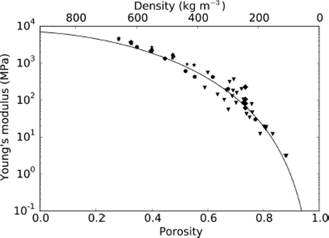
Fig. 1. Krief equation (solid line) fitted and compared to dynamic measurements of Young’s moduli (circles) from Reference JohnsonJohnson (1982). Additional measurements from Reference SmithSmith (1969) are indicated with stars. Theoretical values obtained from numerical modeling of microtomography snow structures are indicated with diamonds and triangles for Reference SchneebeliSchneebeli (2004) and Reference Reuter, Proksch, Loewe, Van Herwijnen and SchweizerReuter and others (2013), respectively.
As data are presented for Young’s moduli rather than bulk modulus in the literature, the bulk moduli resulting from Eqn (3) are converted to Young’s moduli using Eqn (1) and the linear relationship
to express the Poisson’s ratio, ν, of snow as a function of porosity. Figure 2 shows how this function relates to measurements of Poisson’s ratio from Reference BaderBader (1952), Reference RochRoch (1948) and Reference SmithSmith (1969).

Fig. 2. Poisson’s ratio as a function of porosity (solid line) according to Eqn (4) compared to measurements from Reference BaderBader (1952) (dashed lines), Reference RochRoch (1948) (dotted lines) and Reference SmithSmith (1969) (circles).
In combination with the Poisson’s ratio, Eqn (3) can also be used to estimate shear moduli of snow, μ s, as a function of porosity by using the relationship (Reference Mavko, Mukerji and DvorkinMavko and others, 2009)
The shear moduli resulting from Eqns (3–5) are shown in Figure 3 and compared to measurements from Reference JohnsonJohnson (1982) and Reference SmithSmith (1969).

Fig. 3. The shear modulus of snow as a function of porosity (solid line) calculated using Eqns (3–5). Measurements presented by Reference JohnsonJohnson (1982) and Reference SmithSmith (1969) are indicated with diamonds and stars, respectively.
The tortuosity ![]() describing the ‘twisting’ of the actual flow path of the pore fluid compared to a straight line can be estimated based on geometrical considerations as
describing the ‘twisting’ of the actual flow path of the pore fluid compared to a straight line can be estimated based on geometrical considerations as

where s is the so-called shape factor (Reference BerrymanBerryman, 1980). For a packing of equally sized spheres the shape factor is 0.5 and Eqn (6) reduces to

The permeability κ is estimated using the Kozeny–Carman relation

where C is an empirical constant and depends on the material under consideration (Reference Mavko, Mukerji and DvorkinMavko and others, 2009). For sediments the constant is C sediment = 0.003 (Reference Mavko and NurMavko and Nur, 1997; Reference Carcione and PicottiCarcione and Picotti, 2006), but for snow it is an order of magnitude larger, C snow = 0.022 (Reference BearBear, 1972; Reference CalonneCalonne and others, 2012). The grain diameter r can be related to the SSA of snow with the relation
where ρ i is the density of ice. Substituting Eqn Eqn (8) leads to

Due to the compaction and metamorphosis processes inherent to snow it can be assumed that the SSA by itself is a function of porosity (Reference Legagneux, Cabanes and DominéLegagneux and others, 2002; Reference HerbertHerbert and others, 2005). Reference Domine, Taillandier and SimpsonDomine and others (2007) use

where ρ w is the density of water, to relate SSA to snow density. For dry snow, density ρ can be obtained from snow with porosity φ as
Equation (11) yields negative values for the SSA for porosities φ ≤ 0.44. Therefore the relationship is used here only for porosities φ ≥ 0.65. A constant value for SSA of 15 m2 kg−1 is used for lower porosities. In this study, Eqn (11) is intended only to reflect an average trend. Where SSA has significant influence on the analysis, high and low end-member values for SSA are also considered.
The density ρ f, viscosity η and bulk modulus K f of air as the pore fluid of snow are assumed to be constant, i.e. independent of temperature and altitude, and are given in Table 1 (Reference LideLide, 2005).
Table 1. Pore fluid properties of air (Reference LideLide, 2005)

2.2. Phase velocities and plane wave attenuation
A convenient way to obtain closed form solutions for Biot’s (1956b) differential equations is to assume plane wave solutions and substitute these into the differential equations. The complex plane wave modulus is then obtained by solving the resulting dispersion relation (Reference JohnsonJohnson, 1982; Reference PridePride, 2005; Reference CarcioneCarcione, 2007). As, in the poroelastic case, the dispersion relation is a quadratic equation, there are two roots that correspond to the first and second compressional waves. The phase velocity V and the dimensionless quality factor Q, describing the amount of attenuation, can then be obtained from the complex plane wave modulus V c as (Reference O’Connell and BudianskyO’Connell and Budiansky, 1978)

where ω is the angular frequency.
In this study, the solutions of the dispersion relation resulting from Biot’s equations are computed for individual frequencies and porosities. However, if any dissipative effects are ignored and the bulk modulus of the fluid is much smaller than the bulk modulus of the solid matrix it can be shown that the first compressional wave velocity V ∞1 can be expressed as

and the second compressional wave velocity V ∞2 as

where E m = K m + (4/3)μ s is the ice matrix P-wave modulus (Reference Bourbié, Coussy and ZinsznerBourbié and others, 1987, p. 81). Equations (15) and (16) are related to the rigid-frame model and not to Biot’s equations considered in this study. These equations are shown here only to illustrate that the first compressional wave travels mainly in the skeleton and the second compressional wave travels mainly in the fluid. Moreover, these expressions also illustrate that the first compressional wave is most sensitive to the properties of the ice matrix, whereas the second compressional wave is sensitive mostly to properties of the pore space and the pore fluid. Note that the compressional wave velocities for the rigid-frame model, Eqns (15) and (16), are not frequency-dependent.
2.3. Dynamic viscous effects
The fluid flow in the pores of the material has a different character for lower and higher frequencies (Reference BiotBiot, 1956b). For lower frequencies the flow is of Poisson type where the flow is fastest in the center of a pore and reduces gradually in a parabolic shape towards the outside of the pores. For higher frequencies the importance of inertial forces increases. The fluid in the center of the pores flows all with the same velocity like an ideal fluid, while the fluid at the outside of the pores remains attached to the pore walls. In between the two, the so-called viscous boundary layer forms (Reference PridePride, 2005). The transition between low- and high-frequency flow behavior occurs when the viscous boundary layers are smaller than the pore diameter. The frequency at which this transition occurs is called the Biot frequency f Biot and can be computed as (Reference CarcioneCarcione, 2007, p. 270)
Biot’s (1956a) theory is considered valid for frequencies up to the Biot frequency. For higher frequencies Reference Johnson, Koplik and DashenJohnson and others (1987) introduced a frequency-dependent permeability that accounts for the different flow behavior in the low- and high-frequency limit and is often referred to as a frequency correction or the JDK model. Figure 4 shows the Biot frequency for snow based on the relationships between porosity and the involved material properties as presented in Section 2.1, where the permeability further depends on the SSA. To illustrate the variability of Biot’s frequency due to SSA, the Biot frequency is plotted for Eqn (11) which depends on porosity, and for constant end-member values of SSA = 15 m2 kg−1 and SSA = 90 m2 kg−1.

Fig. 4. Biot’s characteristic frequency for snow as a function of porosity based on the relations presented in Section 2.1. The solid line corresponds to SSA as a function of porosity (Eqn (11)). The dashed and dotted lines correspond to the end-member values SSA = 15 m2 kg−1 and SSA = 90 m2 kg−1, respectively.
The results shown in this study are evaluated using the frequency correction (Reference Johnson, Koplik and DashenJohnson and others, 1987). However, for the first compressional wave there are virtually no differences when the frequency correction is neglected. For the second compressional wave the differences are rather low, except for frequencies in the range of the Biot frequency, where moderate differences can be observed.
3. Results
In this section, phase velocities and plane wave attenuation for snow are presented as a function of porosity based on the relationships presented in Section 2.1. Figure 5 shows the predicted phase velocity for the first compressional wave and a frequency of 1 kHz as a function of porosity. The predicted phase velocities are compared to measurements from Reference SmithSmith (1969) and Reference JohnsonJohnson (1982). In addition, the predicted velocity for an individual and a combined variation of 25% in bulk and shear modulus is shown. The velocity strongly decreases with increasing porosity, and the variation of bulk and shear modulus for snow of the same porosity is small compared to the change of velocity over the porosity range.

Fig. 5. Predicted phase velocities for the first compressional wave (solid line) at 1 kHz. Measurements from Reference JohnsonJohnson (1982) and Reference SmithSmith (1969) are indicated with diamonds and crosses, respectively. The dashed and dotted lines are predicted velocities for a 25% variation of matrix bulk modulus and shear modulus, respectively. The dash-dot line corresponds to a 25% variation in both.
The predicted shear velocities at 1 kHz are compared in Figure 6 to measurements by Reference JohnsonJohnson (1982) and Reference Yamada, Hasemi, Izumi and SatoYamada and others (1974). Similar to the first compressional wave, the shear velocity strongly decreases with increasing porosity.

Fig. 6. Predicted shear velocities (solid line) at 1 kHz. Squares and crosses correspond to shear wave velocity measurements from Reference JohnsonJohnson (1982) and Reference Yamada, Hasemi, Izumi and SatoYamada and others (1974), respectively.
The predicted phase velocities of the second compressional wave at 500 Hz as a function of porosity are shown in Figure 7 and are compared to measurements from Reference OuraOura (1952) and Reference JohnsonJohnson (1982). As the pore fluid properties are assumed constant, the phase velocity of the second compressional wave depends almost exclusively on variations in permeability and tortuosity. Variations in frame bulk modulus and shear modulus have virtually no influence on phase velocity and attenuation of the second compressional wave. The tortuosity has a stronger lever on the phase velocity than the permeability, and 30% variation in tortuosity leads to larger changes in phase velocity than a 50% variation in permeability. The phase velocity of the second compressional wave shows little variation with porosity and is mainly sensitive to the geometrical structure of the pore space.

Fig. 7. Predicted phase velocity for the second compressional wave (solid line) at 500 Hz. The dashed and dotted lines correspond to the phase velocities for 30% variation in tortuosity and 50% variation in permeability, respectively. Squares represent velocity measurements from Reference JohnsonJohnson (1982). Crosses correspond to measurements from Reference OuraOura (1952). Note that an increasing tortuosity decreases the velocity while an increase in permeability increases the velocity of the second compressional wave.
The plane wave attenuation for the first compressional wave as a function of porosity is shown for three different frequencies in Figure 8a. It is striking that the attenuation is orders of magnitude higher for light snow with a porosity φ ⪞ 0.8 than for denser snow, such that the variations in the porosity range between φ = 0.55 and φ = 0.8 cannot be resolved and are therefore shown in Figure 8b.

Fig. 8. Predicted attenuation for the first compressional wave as a function of porosity. (b) shows a fragment of (a) for porosities φ < 0.8. The attenuation of the first compressional wave is orders of magnitude higher for light snow than for denser snow.
Homogeneous Biot-type porous materials are known to have a characteristic peak of attenuation (Reference Geertsma and SmitGeertsma and Smit, 1961; Reference Carcione and PicottiCarcione and Picotti, 2006). In Figure 9 these attenuation peaks are shown for snow of different densities. As in Figure 8, the figure is split into two panels to account for the significant difference of attenuation levels for light and dense snow. Peak attenuation shifts towards lower frequencies, and the attenuation level increases with increasing porosity. The same is true for light snow but with considerably higher attenuation levels. Also the peak attenuation frequencies overlap for a porosity range around φ = 0.8.

Fig. 9. Frequency-dependent attenuation for the first compressional wave in (a) medium to dense and (b) light snow. The peak of the attenuation shifts toward higher frequencies for denser snow. Note that the amplitude of the attenuation is orders of magnitude larger for light snow with porosity φ ⪞ 0.8.
Phase velocity and attenuation for the second compressional wave obtained with and without using the frequency correction discussed in Section 2.3 are shown in Figure 10. The dynamic viscous effects are relatively small except in the range of Biot’s frequency, where the phase velocity shows a moderate difference between the solutions including and neglecting a frequency correction (Reference Johnson, Koplik and DashenJohnson and others, 1987). In contrast to the first compressional wave, there is no distinctive difference in attenuation for dense and light snow for the second compressional wave. The sharp bend in phase velocity and attenuation is due to the relationship between porosity and the SSA that was chosen to be constant for φ < 0.65 to avoid the negative values resulting from Eqn (11).

Fig. 10. Phase velocity (a) and attenuation (b) for the second compressional wave for 100 Hz, 1 kHz and 10 kHz. The black lines correspond to solutions including dynamic viscous effects considered by Reference Johnson, Koplik and DashenJohnson and others (1987) while the red lines correspond to solutions of Biot’s (1956a) differential equations without correcting these effects. The symbols denote velocity measurements from Reference OuraOura (1952) and Reference JohnsonJohnson (1982).
The variation of the phase velocity of the second compressional wave due to changes in SSA is shown in Figure 11. For fixed end-member values of SSA = 15 m2 kg−1 and SSA = 90 m2 kg−1 the phase velocity at 500 Hz is plotted with dashed and dotted lines, respectively. The solid line represents the phase velocities resulting from Eqn (11). The variation is larger for denser snow than for light snow, where permeability is less affected by SSA.
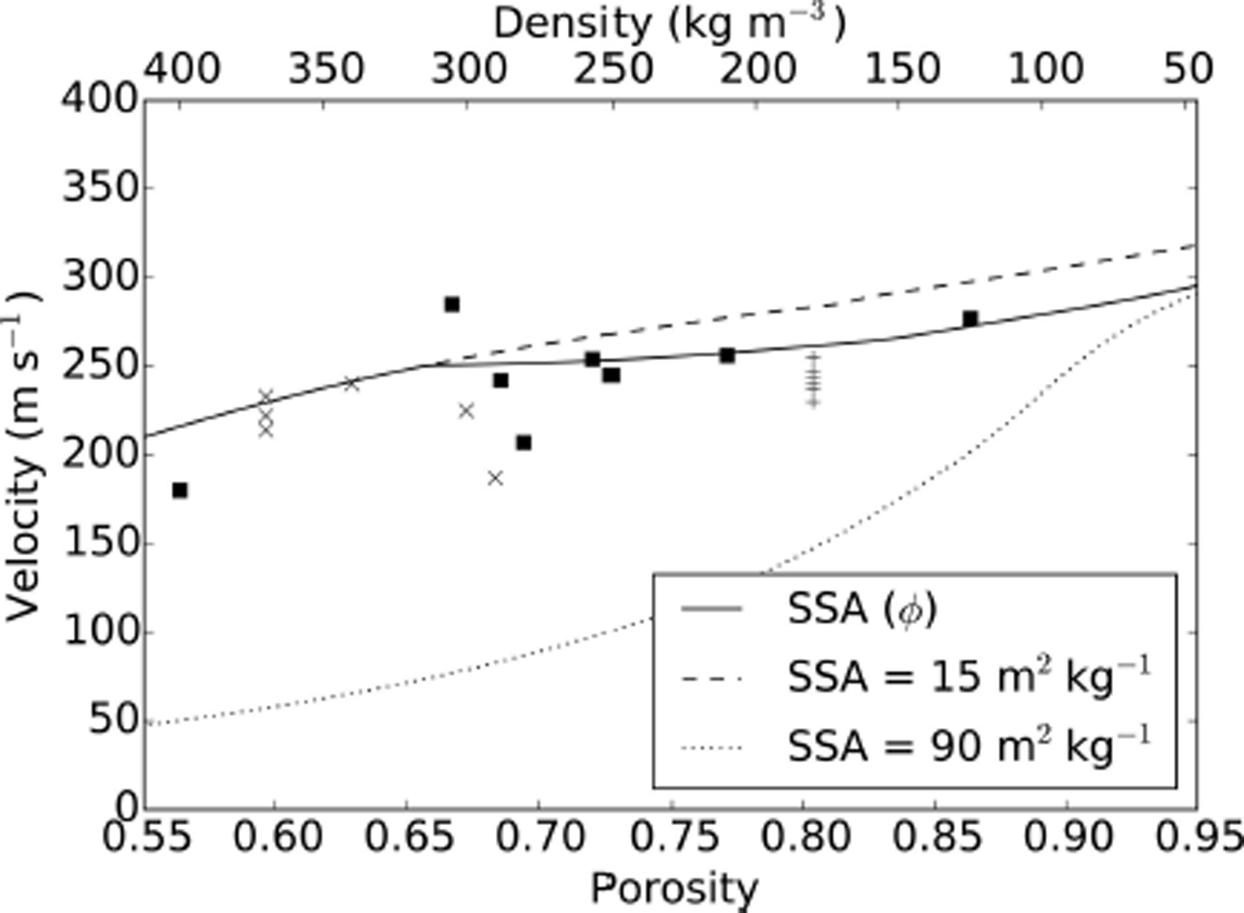
Fig. 11. Predicted phase velocities for the second compressional wave at 500 Hz for a SSA as a function of porosity (solid line) and constant values of SSA = 15 m2 kg−1 (dashed line) and SSA = 90 m2 kg−1 (dotted line). Squares and crosses correspond to measurements from Reference JohnsonJohnson (1982) and Reference OuraOura (1952), respectively.
In Figure 12, attenuation for both compressional waves is shown for constant values of SSA = 15 m2 kg−1 and SSA = 90 m2 kg−1. Also shown is the attenuation for SSA as a function of porosity according to Eqn (11). The attenuation levels of both compressional waves increase with an increase of SSA.

Fig. 12. Predicted attenuation at 500 Hz for the first (a) and second (b) compressional wave as a function of porosity. The dashed and dotted lines correspond to end-member values of SSA = 15 m2 kg−1 and SSA = 90 m2 kg−1, respectively. The solid line corresponds to Eqn (11) and a constant value of SSA = 15 m2 kg−1 for densities above 315 kg m−3.
4. Discussion
4.1. Slow first compressional phase velocity
Compressional phase velocities as a function of porosity compared to measurements presented by Reference JohnsonJohnson (1982) and Reference SommerfeldSommerfeld (1982) are shown in Figure 13. The relations between porosity and the properties of the porous material, especially the strong decrease of matrix bulk modulus with increasing porosity, lead to the peculiarity that the predicted first compressional wave becomes slower than the second compressional wave for light snow with porosity φ ⪞ 0.8. In most materials, the second compressional wave is considerably slower than the first and is therefore sometimes also called the ‘slow’ wave. No measurements of the first compressional wave with a lower phase velocity than the second compressional wave have been reported for snow. However, a first compressional wave with lower phase velocity than the second compressional wave has been observed in high-porosity reticulated foam (Reference Attenborough, Bashir, Shin and TaherzadehAttenborough and others, 2012).

Fig. 13. Predicted velocities for the first (solid line) and second (dashed line) compressional waves as a function of porosity based on empirical relationships for frame bulk and shear modulus, tortuosity and permeability in snow. The dashed lines identify measurements of first compressional waves compiled by Reference SommerfeldSommerfeld (1982), and diamonds and squares represent wave velocity measurements compiled by Reference JohnsonJohnson (1982) for compressional waves of the first and second kind, respectively.
From the plane wave solutions it is not immediately clear that the lower compressional velocity in light snow corresponds to the first compressional wave mode as there are no explicit rules to choose the signs of the square roots. To illustrate that it is indeed the velocity of the first compressional wave that is slower than the phase velocity of the second compressional wave, two numerical simulations solving Biot’s equations of wave propagation in poroelastic materials were performed. In the first simulation the homogeneous poroelastic material corresponds to snow with porosity φ = 0.7, where the first compressional wave is expected to be faster than the second compressional wave. In the second simulation the porosity of the snow is chosen to be φ = 0.9 and the first compressional wave is expected to be slower than the second compressional wave. The relations from Section 2.1 are used to characterize the remaining porous material properties.
For the simulation a pseudo-spectral modeling code was used that solves the acoustic equations in a domain that is located above a second domain where Biot’s (1962) equations are solved. Special care is taken to correctly account for the interface between these two domains, and the code was successfully tested against analytical solutions (Reference Sidler, Carcione and HolligerSidler and others, 2010). To avoid disagreement of the simulations due to varying parameterization of the source characteristics, which is cumbersome in poroelastic materials, the source was placed at 6.9 m from the left boundary and 1.46 m above the air/snow interface at zero vertical distance. The pressure source has a waveform of a Ricker wavelet with a central frequency of 500 Hz. The boundary conditions between the acoustic and the poroelastic domain, which correspond to air and snow, respectively, are assumed to be of the ‘open pore’ type (Reference Deresiewicz and SkalakDeresiewicz and Skalak, 1963). The field variables of the simulation are the velocity of the solid frame, the velocity of the pore fluid relative to that of the solid frame, the stress tensor and the pore pressure. Note that these are particle velocities and should not be confused with the phase velocities discussed before. The first compressional wave has its strongest amplitude in the solid frame velocity field variable, while the second compressional wave has its strongest amplitude in the field variable of the relative fluid velocity.
In Figure 14, snapshots are shown for the two simulations 15.6 ms after triggering the acoustic source. In the acoustic domain, indicated by positive vertical coordinates, the air pressure is shown in all four panels. For the poroelastic domain, indicated by negative vertical coordinates, Figure 14a and c show the horizontal component of the solid frame velocity field that corresponds to the first compressional wave, and Figure 14b and d show the horizontal component of the relative fluid velocity field that corresponds to the second compressional wave. The simulation for snow with porosity φ = 0.7 corresponds to Figure 14a and b, and the simulation for snow with porosity φ = 0.9 corresponds to Figure 14c and d.

Fig. 14. Snapshots after 15.6 ms of a numerical simulation of a pressure source in the air over snowpacks with a porosity (a, b) φ= 0.7 and (c, d) = 0.9. The horizontal components of (a, c) the velocity of the porous frame and (b, d) the velocity of the pore fluid relative to the porous frame are shown. It can be seen that in the highly porous material (φ= 0.9), the first compressional wave (c) is slower than the second compressional wave (d).
In the snapshots, the waves will propagate as rings away from the source. Red and blue indicate positive and negative amplitudes, respectively. The stronger the color, the higher the amplitude. For this example the absolute value of the amplitude of the individual wave fields is only of subordinate relevance; no color bars are indicated. Higher wave velocities of the material will result in larger rings in the snapshots shown for a fixed elapsed time. At the air/snow interface the air-pressure wave will be converted into a reflected air-pressure wave, transmitted first and second compressional waves, as well as a transmitted shear wave. The shear wave is not of interest here and cannot be seen in the presented snapshots. The first and second compressional waves will travel in the poroelastic material with its characteristic velocities. If this velocity is higher than that of the incident wave, the ring in the lower domain will be larger than that in the upper domain (Fig. 14a). If the velocity is less than the speed of sound in the air, the ring in the lower domain will be elliptic with a shorter vertical axis (Fig. 14b–d). Note the particularly short vertical axis in Figure 14c, which indicates an especially low velocity.
Due to the interaction between pore fluid and skeleton, a propagating wave mode will also have an amplitude in field variables that are not its main field variable. For light snow this interaction is relatively strong. Therefore in Figure 14c not only the strong amplitude of the slower first compressional wave with its short vertical axis can be seen, but also a ‘shadow’ of the faster second compressional wave that almost completes the circle of the air pressure wave in the upper domain. From Figure 14 it becomes clear that in the simulation of light snow the second compressional wave is faster than the first compressional wave.
4.2. Increased sound absorption of light snow
The attenuation levels of the first compressional wave differ significantly for light snow with a porosity φ ⪞ 0.8 and snow with a lower porosity. This separation corresponds roughly to a separation between freshly fallen and aged snow (Reference Judson and DoeskenJudson and Doesken, 2000). Between the two porosity ranges, the attenuation vanishes completely as the two wave modes have the same velocity and the viscous effects leading to attenuation are not in effect. The sound absorption above ground is a complex combination of effects involving, amongst others, the interference of incident and reflected waves, the reflection coefficient, geometrical spreading, as well as surface and non-geometrical waves (Reference EmbletonEmbleton, 1996). However, it is clear that if the reflection coefficient of the ground decreases, the sound level above the ground also decreases (Reference WatsonWatson, 1948; Reference Nicolas, Berry and DaigleNicolas and others, 1985). Due to the high porosity of snow and the open pore boundary conditions, the pressure of the air above the snowpack interacts mainly with the air in the pore space and little energy is transmitted into the ice frame. As the velocity of the second compressional wave is almost equal to the velocity of the air above the snow, there is almost no impedance contrast that would lead to a reflection. The low velocity of the first compressional wave in snow with porosity φ > 0.8 and the corresponding higher attenuation further decreases the impedance contrast and also reduces the contribution of refracted waves.
5. Conclusions
A method to predict phase velocities and plane wave attenuation of acoustic waves as a function of snow porosity has been presented. It is based on Biot’s (1956a) model of wave propagation in porous materials and uses empirical relationships to assess tortuosity, permeability, bulk and shear moduli as a function of porosity. The properties of the ice frame of the snow and air as the pore fluid are assumed constant. The method is not restricted to porosity, as a single degree of freedom and additional information on SSA or any of the other properties characterizing a Biot-type porous material can be readily incorporated.
For light snow with a porosity φ ⪞ 0.8 the peculiarity is found that the velocities of the first compressional wave are slower than the phase velocities of the second compressional wave which is commonly referred to as the ‘slow’ wave. Such a reversal of the velocities of the compressional waves has been observed in reticulated foam before and is due to the weak structure of the ice matrix in fresh and light snow. The wave velocity reversal is a relatively sharp boundary for the attenuation level of the first compressional wave, which is orders of magnitude larger for highly porous snow. This finding is in accordance with the well-known observation that freshly fallen snow absorbs most of the ambient noise, while after a relatively short time this absorbing behavior vanishes.
The first compressional wave is sensitive mainly to matrix and shear bulk moduli. A variation of ∼25% in both shear and matrix bulk moduli can characterize the variability in measured velocities. The attenuation of the second compressional wave decreases with increasing porosity and is considerably higher than for the first compressional wave. Also frequency dependence of the attenuation is considerably more distinct for the second compressional wave. The velocity of the second compressional wave depends strongly on tortuosity, permeability and the related SSA. The variation of measured wave velocities for the second compressional wave can be obtained by altering the tortuosity by ∼30% or by altering the permeability by ∼50%.
This method is a basic requirement for numerical modeling of acoustic wave propagation in snow, which makes it possible, for example, to assess the design of acoustic experiments to probe for snow properties or to assess the role of acoustic wave propagation in artificial or skier-triggered snow avalanche releases.
Further research will address the presence of liquid water in the pore space, a more complete analysis of sound absorption above snow of varying porosity, and numerical simulations of explosive avalanche mitigation experiments.
Acknowledgements
This research was founded by a fellowship of the Swiss National Science Foundation. I thank editors John Glen, Perry Bartelt, chief editor Jo Jacka, reviewer Henning Löwe and two anonymous reviewers for constructive comments and suggestions that helped to improve the manuscript.


