


1. Introduction
Glacier inventories exist for most regions of the world (e.g. Bajracharya and Shrestha, Reference Bajracharya and Shrestha2011; Pfeffer and others, Reference Pfeffer2014; Nuimura and others, Reference Nuimura2015; Mölg and others, Reference Mölg, Bolch, Rastner, Strozzi and Paul2018; Scherler and others, Reference Scherler, Wulf and Gorelick2018; Herreid and Pellicciotti, Reference Herreid and Pellicciotti2020). These are generally based upon satellite imagery (Racoviteanu and others, Reference Racoviteanu, Paul, Raup, Khalsa and Armstrong2009; Shukla and others, Reference Shukla, Arora and Gupta2010). Clean ice can be mapped relatively easily, notably using thermal bands, though the threshold used to define ice cover needs calibration as they can vary both spatially and temporally (Veettil and others, Reference Veettil, Bremer, Grondona and De Souza2014; Robson and others, Reference Robson2015; Haireti and others, Reference Haireti, Tateishi, Alsaaideh and Gharechelou2016). However, mapping debris covered ice remains a challenge (Bolch and Kamp, Reference Bolch and Kamp2005; Raup and others, Reference Raup2007; Racoviteanu and others, Reference Racoviteanu, Paul, Raup, Khalsa and Armstrong2009; Mölg and others, Reference Mölg, Bolch, Rastner, Strozzi and Paul2018). Mountain glaciers can develop significant debris cover that can substantially modify glacier melt processes and response to climate warming (Nicholson and Benn, Reference Nicholson and Benn2006; Jouvet and others, Reference Jouvet, Huss, Funk and Blatter2011; Scherler and others, Reference Scherler, Bookhagen and Strecker2011; Zhang and others, Reference Zhang, Fujita, Liu, Liu and Nuimura2011; Pratap and others, Reference Pratap, Dobhal, Mehta and Bhambri2015; Rowan and others, Reference Rowan, Egholm, Quincey and Glasser2015; Vincent and others, Reference Vincent2016; Nicholson and others, Reference Nicholson, McCarthy, Pritchard and Willis2018; Ferguson and Vieli, Reference Ferguson and Vieli2021).
Mapping debris covered ice from satellite imagery has made use of two primary approaches. The first is geomorphometric (e.g. Paul, Reference Paul2003; Paul and others, Reference Paul, Huggel and Kääb2004; Bolch and Kamp, Reference Bolch and Kamp2006; Shukla and others, Reference Shukla, Arora and Gupta2010; Bhardwaj and others, Reference Bhardwaj, Joshi, Singh, Sam and Gupta2014; Veettil and others, Reference Veettil, Bremer, Grondona and De Souza2014) where debris in ice marginal zones is classified as ice cored if local slope is below a certain threshold (the critical slope angle for debris movement). This may be problematic in some regions, such as where the transition from a glacier margin to an unglaciated region is gentle but still relatively debris free (Paul, Reference Paul2003; Bolch and Kamp, Reference Bolch and Kamp2006). In addition, no detectable change in surface slope may occur at the interface between clean-ice and debris-cover (Bhambri and others, Reference Bhambri, Bolch and Chaujar2011); post-depositional sedimentation by mass movement, a commonly found process in the polygenetic environment of the Himalaya (Benn and Owen, Reference Benn and Owen2002; Bhambri and others, Reference Bhambri, Bolch and Chaujar2011), may cause confusion (Bhambri and others, Reference Bhambri, Bolch and Chaujar2011); and the available topographic data may not have the right resolution (Bolch and Kamp, Reference Bolch and Kamp2006; Racoviteanu and others, Reference Racoviteanu, Paul, Raup, Khalsa and Armstrong2009).
One alternative is to use differences in temperature between debris-covered ice and the temperature of the surrounding ice-free zones. Taschner and Ranzi (Reference Taschner and Ranzi2002) analyzed the surface temperature and physical properties of both debris layers on glaciers and non ice containing zones (debris, rocks, grass) using ground measurements obtained for temperature and heat flux. They found significant temperature differences between debris-covered ice and other land surfaces with higher temperatures on average for surfaces without underlying ice. Amschwand and others (Reference Amschwand2021) recorded such differences to a debris thickness of 5 m. Subsequent studies have exploited this observation in satellite data. Scherler and others (Reference Scherler, Wulf and Gorelick2018), Herreid and Pellicciotti (Reference Herreid and Pellicciotti2020) and Fleischer and others (Reference Fleischer, Otto, Junker and Hölbling2021) have used the proportion of near infrared (NIR) and shortwave infrared (SWIR) to map debris cover on glaciers. Stewart and others (Reference Stewart2021) attempted to estimate debris thickness on glaciers using 60 m × 60 m Landsat Enhanced Thematic Mapper + data resampled to 30 m by 30 m. Herreid (Reference Herreid2021) used ASTER data processed to give surface kinetic temperature at a 90 m resolution and then used an unmixing approach to estimate the extent of debris-covered ice within a pixel, emphasizing the need for downscaling of the generally coarse thermal bands especially for mountain glaciers.
There are three issues that follow from these thermal band satellite based approaches. First, with very thick debris cover, the signal of ice temperature will diminish (Racoviteanu and others, Reference Racoviteanu, Paul, Raup, Khalsa and Armstrong2009; Shukla and others, Reference Shukla, Arora and Gupta2010) resulting in zones of debris-covered ice being classed as nonglacier. We assume that the importance of this problem is likely to increase with rapid glacier retreat, leading to potentially extensive areas of debris-covered ice that may be patchy and/or disconnected from the glacier itself. It emphasizes the need for further research to identify the limits of satellite-based estimation of debris-cover thickness. Second, following from the typical resolutions reported above, satellite-based studies have struggled to map small glaciers. Herreid and Pellicciotti (Reference Herreid and Pellicciotti2020), for instance, excluded glaciers <1 km2 even if for some mountainous regions a large proportion of glaciers fall in this class (Maharjan and others, Reference Maharjan2018). One solution could be to downscale coarser thermal using higher resolution panchromatic bands as has been done in other applications (Choi, Reference Choi2006; Aiazzi and others, Reference Aiazzi, Baronti and Selva2007; Choi and others, Reference Choi, Yu and Kim2010; Jung and Park, Reference Jung and Park2014; Rai and Mukherjee, Reference Rai and Mukherjee2021). Third, it is not yet clear whether or not a single index can map ice-covered debris regardless of the geological composition of such debris. If weathering processes lead to significant accumulation of fine-grained sediments on debris-covered glaciers then the debris cover will have small void spaces. This may result in greater capacity for water retention leading to wet surfaces (Juen and others, Reference Juen, Mayer, Lambrecht, Wirbel and Kueppers2013; Blum and others, Reference Blum, Nortcliff and Schad2018) with different thermal properties to dry ones. As water and ice affect the thermal properties of a debris layer (Giese and others, Reference Giese, Boone, Wagnon and Hawley2020) more than one index may be needed to capture the spatial extent of debris-covered ice fully.
Given that debris cover remains a major cause of uncertainty in quantifying the retreat of glaciers in mountain regions (Scherler and others, Reference Scherler, Bookhagen and Strecker2011), there is a need for further development and testing of indices that can be used to map debris-covered ice in mountain regions, notably ones that can address the three issues identified above. Thus, the primary aim of this paper is to develop indices for mapping ice and debris-covered ice extent for mountainous regions that; (a) yield sufficient spatial resolution for mapping of valley-confined glaciers, including those < 1 km2 in size; (b) are sensitive to geological controls on the caliber of accumulated sediment; (c) are suitable for long-term analyses so as to quantify change; and (d) use freely-available datasets.
The focus is on Afghanistan in the western part of Hindu Kush Himalaya where there remains only a poorly-developed understanding of the cryosphere despite its impact on both water resources and environmental hazards (Shokory and others, Reference Shokory, Schaefli and Lane2023). Most glaciological studies in Afghanistan are for the period 1965 to 1980 and are in Russian, Dutch and very occasionally English, and most are not available online (Shroder and Bishop, Reference Shroder, Bishop, Williams and Ferrigno2010). In 1980, Shroder initiated a glacier inventory for Afghanistan supported by the U.S. Geological Survey using Landsat-3 satellite imagery (40 m ground resolution), and field observations (Shroder and Bishop, Reference Shroder, Bishop, Williams and Ferrigno2010). This research identified about. 3000 separate glaciers in Afghanistan with an estimated area of about 2700 km2 (Shroder, Reference Shroder1980; Shroder and Bishop, Reference Shroder, Bishop, Williams and Ferrigno2010; Shroder and Ahmadzai, Reference Shroder and Ahmadzai2016). A glacier inventory of Afghanistan was published by the Afghanistan Ministry of Energy and Water and International Centre for Integrated Mountain Development using satellite Landsat imagery (Maharjan and others, Reference Maharjan2018). Glaciers were mapped using semi-automatic object-based image analysis methods and debris-covered ice was mapped using slope thresholds (0–24°). Maharjan and others (Reference Maharjan2018) identified 3782 glaciers, covering a total area of about. 2540 km2 (excluding glaciers with an area of less than 0.01 km2) concentrated at elevations between 3200 and 6900 m a.s.l. Thus, a subsidiary aim of the work is to produce a new glacier inventory for Afghanistan. As our method leads to one of the first inventories that can map very small (<1 km2) glaciers, we seek to identify the regional-scale, systematic controls that explain spatial variation in debris-covered ice extent for Afghanistan using our inventory.
2. Study area
Afghanistan is a mountainous country located in the subtropics, extending from 29°21′N to 38°30′N latitude and from 60°31′E to 75°E longitude (Gopalakrishnan, Reference Gopalakrishnan1982) (Fig. 1). It has an arid and semi-arid continental climate, characterized by temperature and precipitation regimes characteristic of deserts, steppe and highland environments (Humlum and others, Reference Humlum, Køie and Ferdinand1959; Shroder, Reference Shroder2014). It has four main glacier regions (Fig. 1). We aim to produce a glacier inventory for all of Afghanistan. To support this work, we looked at two cases within Afghanistan in greater detail.

Fig. 1. Afghanistan showing the four glacier regions and their climatic zones (inset) based on the Köppen–Geiger climate classification (Peel and others, Reference Peel, Finlayson and McMahon2007) modified to include Dsa - M (Monsoonal influence) following Shroder (Reference Shroder2014).
We undertook field data collection at the Mir Samir Glacier (Fig. 1) for index calibration and validation, which is the only glacier monitored by the Ministry of Energy and Water (MEW) of Afghanistan. This glacier is located at 70.171°N longitude and 35.596°E latitude (Fig. 1). Its highest altitude is 5060 m and it extends over a distance of 2.9 km to 4200 m altitude. The Mir Samir Glacier was mostly debris-covered in its snout zone, with some large boulders present. The proglacial margin also contains debris-covered ice. The geology around and under the glacier varies from slightly metamorphosed sedimentary rocks to hard gneisses and schists (Gilbert and others, Reference Gilbert, Jamieson, Lister and Pendlington1969). This glacier was the primary focus of the first index we develop for mapping debris cover.
A second case, the Noshaq glacier range (Fig. 1) was also studied more intensively, albeit without a field visit. This glacier range was identified during the study as having debris-covered ice that was not being detected using our first index and so became the focus of the second index we developed. The Noshaq glacier range was studied in detail by Shroder (Reference Shroder1978) (Fig. 1, Fig. S1, Supplementary Material). It contains one of the longest and largest glaciers in Afghanistan, starting from Noshaq peak, the highest peak in Afghanistan (7492 m) and extending for 14 km to an elevation of about 3580 m (Shroder, Reference Shroder1978) (location 36° 25′ N, 71° 47′ E).
3. Methodology
The approach makes use of freely available imagery from the Landsat 8 Operational Land Imager. The spatial resolution of its thermal bands is 90–120 m which creates particular uncertainty where clean ice and debris-covered ice are in juxtaposition (Bhambri and others, Reference Bhambri, Bolch and Chaujar2011; Kääb and others, Reference Kääb2014) or glaciers are small in size (<1 km2). Thus, the two indices developed herein aim to improve the spatial resolution of thermal-based mapping and to resolve debris-covered ice where there is only a weak thermal signal.
3.1 Datasets
Data were obtained for ten L8 image tiles for the end of the 2016 ablation season (primarily in September) from http://earthexplorer.usgs.gov/ (Fig. S2, Supplementary Material), and on dates with no seasonal snow or cloud cover present in the scenes. The indices we developed used bands directly provided by Landsat 8; blue-B2, near infrared (NIR)-B5, shortwave infrared (SWIR)-B6, panchromatic (PAN)-B8 and thermal (TIR)-B10. The B2, B5 and B6 bands have 30 m resolution, the B8 band 15 m resolution and the B10 band 100 m resolution that supplied already downscaled to 30 m. To correct for top of atmosphere reflectance, before all further analyses, we applied the radiometric rescaling coefficients provided in the associated metadata files delivered with the Landsat Level-1 NIR and SWIR products. We address the correction of PAN and TIR bands below.
Digital elevation models (DEMs) with resolutions of 5 m or 10 m (according to region) were provided by the Department of Statistics, Ministry of Agriculture Irrigation and Livestock of Afghanistan (MAIL, 2020). In areas where no Afghan DEMs were available we used 30 m resolution DEMs downloaded from the ALOS global digital surface model (ALOS, 2022). The Russian geological vector map of Afghanistan and high resolution (0.29 m) 2016-RGB images were obtained from Ministry of Mines and Petroleum of Afghanistan (MoMP, 2020).
3.2 Indices for mapping ice and debris cover
To map bare ice, we used the NIR to SWIR band ratio (Paul and others, Reference Paul, Kääb, Maisch, Kellenberger and Haeberli2002; Reference Paul, Huggel and Kääb2004; Taschner and Ranzi, Reference Taschner and Ranzi2002; Paul, Reference Paul2003; Bolch and Kamp, Reference Bolch and Kamp2005; Shukla and others, Reference Shukla, Arora and Gupta2010; Bhardwaj and others, Reference Bhardwaj, Joshi, Singh, Sam and Gupta2014; Veettil and others, Reference Veettil, Bremer, Grondona and De Souza2014). While methods for mapping debris-covered ice are available (see Supplementary Material), we develop a new index based upon a combination of L8 TIR and PAN bands. The principle behind this combination is that the TIR band is the one most likely to contain the thermal signal that allows identification of thicker debris layers. However, the L8 supplied TIR band is coarser (30 m). The PAN band is 15 m and, while theoretically less sensitive to thermal properties, it provides a means of downscaling the coarser TIR band to the resolution needed for mountain valley glaciers. This was done by assigning to each PAN value the nearest TIR value. The structural characteristics of debris-covered ice lead to a unique texture and panchromatic data have the potential to detect it (Bishop and others, Reference Bishop, Shroder and Ward1995).
The PAN band has a reversed reflectance value (lower to higher) over debris to ice compared to TIR (higher to lower) (Fig. S3, Supplementary Material). On this basis we define a Normalized Difference Supraglacial Debris Index (NDSDIc1):
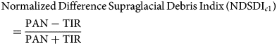
During application we noted for a small number of glaciers in certain geological regions where the NDSDIC1 suggested no debris-covered ice when there was likely to be ice present. Looking at the Russian geological map of Afghanistan (MoMP, 2020), we noted such regions were associated with detrital sedimentary rocks (mainly sandstone, siltstone, argillite, shale) (Shroder, Reference Shroder1980; Shroder and Bishop, Reference Shroder, Bishop, Williams and Ferrigno2010) which are highly erodible and result in smaller grain-size debris and likely wetter sediment. As the visible to near infrared single band ratio has been used previously to detect moist surfaces (Lobell and Asner, Reference Lobell and Asner2002; Amani and others, Reference Amani, Parsian, MirMazloumi and Aieneh2016), we use this to define a second index to capture ice covered by small-grained and moist debris:

3.3 Application of the indices
The indices were applied using the eCognition software (Trimble ©). Figure 2 shows the workflow for applying the indices and key steps are illustrated in Supplementary Material, Figure S4.

Fig. 2. Methodological steps used in the study. The letters shown link to Supplementary Material Figures S4a to S3i, DEMs used for each image tiles are showed in Supplementary Material Figure S2.
As an initial step, radiometric calibration was performed to convert digital numbers (DNs) for NIR and SWIR bands to reflectance values to map bare ice. Radiometric calibration and atmospheric correction was necessary for the NIR and SWIR bands (Fig. S4b, Supplementary Material). Radiometric calibration decreased the numerical range of NDSDI values during debris-covered ice mapping and also caused loss of resolution (Fig. S5, Supplementary Material). Thus, we used the original band DNs in (1) and (2).
Research has shown that misclassifications of pixels as debris-covered ice (e.g. Supplementary Material, Fig. S4d) can occur where there are steep debris-free slopes (Zollinger, Reference Zollinger2003) and cold-water bodies. Following others (e.g. Bolch and others, Reference Bolch, Buchroithner, Kunert and Kamp2007; Bhambri and others, Reference Bhambri, Bolch and Chaujar2011; Bhardwaj and others, Reference Bhardwaj, Joshi, Singh, Sam and Gupta2014; Veettil and others, Reference Veettil, Bremer, Grondona and De Souza2014), we first applied a local slope threshold of 37° on a pixel basis to remove bare rock surfaces but this did not eliminate the problem. Hence, we merged pixels into zones (clean ice, debris-covered ice, ice-free) and then calculated the mean slope of each debris-covered ice zone. The average value of slope was calculated by zone and those zones with slopes >24° were reclassified as ice-free.
Even with these thresholds, some areas of supposed debris-covered ice remained that were unlikely to be correct as they were too low in altitude compared with known glacier snout margins (Fig. S4e, Supplementary Material). For this we identified a minimum altitude threshold that differs based on each region (3500–4000 m a.s.l). Shadowed snow patches and bedrock misclassified as debris-covered were identified by using a minimum area (<0.01 km2) of debris cover (following Tielidze and others, Reference Tielidze2020). Lastly, some snow cover area was mapped as ice (e.g. Fig. S4i, Supplementary Material) and more recent imagery was used to identify and to remove such errors.
In summary, the following parameters need to be calculated and calibrated in our analyses: (1) a threshold for the NIR/SWIR ratio to identify clean ice; (2) threshold ranges for the two new indices of debris cover ice NDSDIc1 and NDSDIC2; (3) a slope threshold applied to merged debris-covered glacier zones to remove those erroneously identified as debris-covered ice; (4) a minimum altitude threshold; and (5) a minimum area threshold.
3.4 Calibration, validation and inventory comparison
Our approach to calibration and validation had six steps. First, we visually identified plausible parameter values and ranges by looking across a set of glaciers using the high resolution RGB image. For all parameters except the two NDSDI indices, the result was a set of plausible parameter values. For the two NDSDI indices it was plausible parameter ranges.
Second, we formally acquired field data for the Mir Samir glacier (Fig. 1) in September 2020, and randomly-selected a subset of this dataset to calibrate the ranges for the NDSDIc1 index (Eqn (1)). Security issues meant we could only map one glacier, and even then we had to undertake field data collection with the support of armed guards. The Mir Samir Glacier is mostly debris-covered at its snout, with bigger boulders and potentially ice-cored debris in the proglacial margin. A total of 219 GPS points were collected under a stratified-random sampling approach using a Garmin GPSMAP 64s GPS (±3 meter positional uncertainty) from three ground types; clean ice zones, zones of debris-covered ice and nonice zones (Fig. S6, Supplementary Material). Thin and partially debris-covered ice was determined visually. Thicker debris-covered ice was identified by the presence of ice under large boulders. The full dataset was randomly divided in half for calibration and validation.
Third, as the field validation site for NDSDIc1 did not include fine-grained sedimentary debris-cover, and required to validate NDSDIc2 debris-cover classifications, we turned to the Noshaq range (Fig. 1). High resolution MoMP (2020) imagery was used to visually identify debris-covered ice by the presence of supraglacial ponds and crevasses (Bodin and others, Reference Bodin, Rojas and Brenning2010; Mölg and others, Reference Mölg, Bolch, Rastner, Strozzi and Paul2018). We then randomly selected points from ice-covered, debris-covered ice and nonice zones, which were also randomly separated into calibration and validation datasets.
Fourth, in order to assess the transferability of our approach, we manually mapped four other debris-covered glaciers in Afghanistan from the high resolution RGB imagery. We also tested our approach at the Santopath Glacier in the central Himalaya, India and the Khumbu Glacier in Nepal (Miles and others, Reference Miles2018). Both sites have reliable published maps of debris-covered-ice. We applied our methodology (Fig. 2) to these glaciers.
Finally, we compared the glacier outlines of our study with datasets published by (1) Maharjan and others (Reference Maharjan2018) that used only a slope threshold >24o to identify debris-covered ice and the NDSI index for clean ice; (2) Scherler and others (Reference Scherler, Wulf and Gorelick2018) who used the Randolph Glacier Inventory (RGI) version 6.0 outline and then used 2013–2017 Landsat and 2015–2017 Sentinel optical satellite images to map where glaciers were debris-covered; and (3) Herreid and Pellicciotti (Reference Herreid and Pellicciotti2020) who used the NIR/SWIR satellite band ratio to map debris cover and clean ice using Landsat data for 2013–2015. The outlines provided by Herreid and Pellicciotti (Reference Herreid and Pellicciotti2020) came with on-line available datasets and so we also assessed their approach quantitatively for our 8 glaciers (two Afghan glacier used for calibration and validation; four additional glaciers in Afghanistan used for validation; and the Satopanth and Khumbu glaciers) where the datasets were available.
For both calibration and validation we used an error matrix approach (Congalton and Green, Reference Congalton and Green2019) as used to evaluate land-cover classifications based on reference data (Foody, Reference Foody2002; Congalton and Green, Reference Congalton and Green2019). We calculated classical error statistics (total, user and producer accuracies) but also the Kappa statistic as the latter corrects accuracy assessments for chance agreement between classes (Lillesand and others, Reference Lillesand, Kiefer and Chipman2015). The commission errors define the user accuracy (i.e. the reliability of information derived from the classification; Story and Congalton, Reference Story and Congalton1986) and so they can be used as proportional uncertainties to calculate uncertainty in mapped areas.
3.5 Inventory and exploration of controls on debris cover
We applied our methodology (Fig. 2) to all glaciers in Afghanistan to produce a new inventory. We then explored controls on debris cover percentage using Principal Components Analysis (PCA; Table 1). Catchments were identified using watershed delineation in ArcGIS at the outlet of each glacier. Catchment boundaries were then used to determine catchment area (1), and mean slope (2). Glacier length (3) was calculated following the Machguth and Huss (Reference Machguth and Huss2014) method that determines and measures the centerline of the glaciers. However, for smaller glaciers (<0.07 km2) we found that the method miscalculated glacier length as such glaciers often had their long axis tangential to the glacier surface slope rather than along it. For such glaciers, we used ArcGIS to calculate the longest distance between upper and lower points of the glacier. Herreid and Pellicciotti (Reference Herreid and Pellicciotti2020) suggested determining glacier width as the linear distance orthogonal to glacier flow at the widest location of the main centerline. However, considering the complexity of glaciers in Afghanistan (Fig. 3) this method may not represent glacier width correctly. Thus, we calculated an effective glacier width (4) for individual glaciers by dividing glacier area to the glacier length. The debris influence area (5) was determined by intersecting each glacier outline with the glacier catchment outline (using the intersect toolbox in ArcGIS) and defining the influence area as that having altitudes higher than the lowest altitude of debris-covered ice. The DEM was used with the glacier boundaries to calculate glacier mean elevation (6), glacier elevation range (7) and glacier mean slope (8) using the zonal statistic tool in ArcGIS. The geological information for each glacier (9) was extracted from the geological map of Afghanistan provided by the Ministry of Mines and Petroleum of Afghanistan (MoMP, 2020). The geological information consists of 27 geological type grouped into 6 geological categories. In addition, the Köppen-Geiger climate classification (Peel and others, Reference Peel, Finlayson and McMahon2007) was used to represent the climate characteristics of the glaciers.

Fig. 3. Comparison of the index results for Afghanistan glaciers 1 to 4 and the Satopanth and Khumbu glaciers with those using other indices. Blue and red outlines used as reference outlines.
Table 1. Glacier parameters derived for the multivariate analysis

Due to potential inter-correlation between these variables, PCA was used to reduce this dataset to a set of linearly independent principal components (PCs) that were then used to explain the statistical controls on debris cover (Gupta and others, Reference Gupta, Tiwari, Saini and Srivastava2013; Ghosh and others, Reference Ghosh, Pandey and Nathawat2014). First, we standardized the data by dividing each variable by its standard deviation. Second, the PCA was applied and the variance and factor loadings were calculated (Jensen, Reference Jensen1996; Ghosh and others, Reference Ghosh, Pandey and Nathawat2014). Orthogonal rotation (orthomax) that maximizes a criterion based on the variance of the loadings was used to simplify the interpretation of the resulting factors, and to ensure that the components remained pairwise uncorrelated for subsequent linear modeling. We used a 5% contribution to the original data variance as the cut off for retaining a component. We then interpreted each component with respect to its loadings.
Finally, we established relationships between percentage of debris cover and the new PCs. For this purpose, we used an optimizing stepwise regression where components were added to the model in order of decreasing importance provided that their individual contribution to the total explanation of the model was significant at p < 0.05. We undertook this modeling for both the entire dataset, but also the dataset divided in two ways: by climatic zones and by geological classes.
4. Results
4.1 Index calibration, validation and comparison
For the clean ice NIR/SWIR threshold, visual comparison of results with the imagery suggested that a value of NIR/SWIR ⩾3 appeared to map clean ice effectively. The mean zonal slope for the removal of zones (not pixels) misclassified as debris-covered ice was 24o. We found that an elevation threshold altitude of <3500 m for regions 2, 3 and 4 and altitude <4000 m for region 1 (Fig. 1) was appropriate for the minimum altitude condition (Supplementary Material, Fig. S4 e,h). Finally, we removed zones classified as glacier or debris-covered glacier <0.01 km2 if detached from ice and/or debris-covered ice (Supplementary Material, Fig. S4 e,i). The visual analysis suggested the following two parameter ranges for debris covered ice 0 > NDSDIC1 ⩾−0.32; and 0.88 ⩾ NDSDIC2 ⩾ 0.70.
Based on the ground observations from glacier, pixels with NDSDIC1⩾−0.37 were classified as debris-covered and was optimal, therefore adopted for this study. The calibration accuracy assessment (Table 2) gave very encouraging results; the overall accuracy was 0.98 and the Kappa coefficient was 0.91. For the second index, a range of 0.92 ⩾ NDSDIC2 ⩾ 0.70 was chosen to maximize the accuracy of the approach. The overall accuracy for the Noshaq glacier range was 0.92 and the Kappa coefficient for both clean ice and debris-covered ice was 0.91 (Table 2).
Table 2. Calibration results for the Mir Samir and Noshaq glaciers
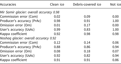
Table 3 shows the validation results for the Mir Samir and the Noshaq glaciers and also for the four other glaciers considered in Afghanistan and the two outside of Afghanistan (Fig. S7 Supplementary Material). The results are encouraging as there is only a very slight degradation in the overall accuracy and the Kappa coefficient in transferring the calibrated index both within and between glaciers.
Table 3. Validation results and comparison with the Herreid and Pellicciotti (Reference Herreid and Pellicciotti2020) index
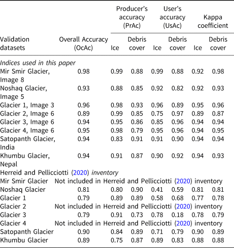
For the Afghan glaciers 1–4 (Fig. 3) the extent of debris-covered ice in the glacier marginal zone is revealed by supraglacial ponds and crevasses and these zones tend to be missed in part by other inventories as compared with our method (Fig. 3, Glacier 2). Compared with the Herreid and Pellicciotti (Reference Herreid and Pellicciotti2020) approach, we obtained higher Kappa coefficient accuracy with our method for Glacier 1 (0.95 and 0.96 for clean ice and debris-covered ice respectively as compared to 0.77 and 0.78 respectively) mainly due to better estimation of ice presence in the margin of the glacier (Fig. 3, Glacier 1). Similarly, for Glacier 3, debris cover ice was missed around the terminus and margins by the Herreid and Pellicciotti (Reference Herreid and Pellicciotti2020) index resulting also in lower accuracies and Kappa coefficients (Table 3).
Our method also shows higher accuracies level for those glaciers outside of Afghanistan in the Himalaya (Table 3). We obtained 0.94 Kappa accuracy for clean ice and debris cover ice for both glaciers using our method. The Herreid and Pellicciotti (Reference Herreid and Pellicciotti2020) index gives lower values for both the Satopanth glacier and the Khumbu glacier.
4.2 Glacier inventory
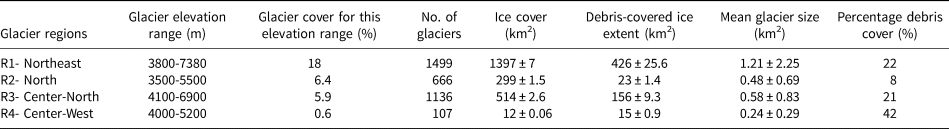
We identified (Table 4) 3408 glaciers which, considering those ⩾0.01 km2, sums to 2,222 ± 11 km2 of ice cover, 619 ± 40 km2 of debris-covered ice and glacier surface areas up to 21.2 km2. Differences in the number of glaciers by region varied reflecting different climatic, elevation and geological zones. Region 1 has the highest number of glaciers, with a larger mean and variability of glacier area (1.21 ± 2.25 km2). The percentage of debris-covered ice is highest in Region 4 (42%) where there are also fewer and smaller glaciers. Regions 1, 2, 3 and 4 have 69%, 4%, 25% and 2% of the total debris cover. The glaciers differ markedly in altitudinal range (Table 4).
Table 4. Summarize the glacier inventory of Afghanistan for 2016
There is a clear regional association in both size and debris cover (Fig. 4) and these associations were significant (Kruskal–Wallis H, p < 0.05).

Fig. 4. Box plots of glacier ice cover size a) and percentage debris cover b) at four regions. The upper and lower box margins mark the 75th (Q75) and the 25th (Q25) quartiles respectively, with the mid box line showing the median. The whiskers show the extremes of the data (maximum and minimum) except for situations where outliers are present, defined as either Q75 + 1.5(Q75−Q25) for the maximum and Q25−1.5(Q75−Q25) for the minimum.
Hypsometric distributions (Fig. 5) suggest that glaciers are distributed between 3500 and 7380 m a.s.l, but that debris-covered ice is limited to altitudes below 5500 m. There is between region-variability. Glaciers in Region 1 and 3 concentrate on 5000 m a.s.l altitude and Region 2 and 4 on 4500 m a.s.l. Comparing glacier elevation ranges, Region 1 and 3 are at higher elevations than Region 2 and 4 (Table 4). This shows a clear signal of altitudinal effects on glacier distribution in Afghanistan.

Fig. 5. Hypsometric distribution curve of glaciers (a) and debris cover (b) in percentage grouped in bins of 100 m and by region.
Regions 1 and 3 tend to have larger glaciers than 2 and 4 (Fig. 6). The percentage debris-covered ice shows significant correlation with glacier size; smaller glaciers have more debris-covered ice than larger glaciers, notably for Regions 1, 2 and 3. The relation is nonlinear to varying degrees and heteroscedastic (Fig. 5), small glaciers in Region 2 and 3 in particular having disproportionately higher percentage debris cover but also a greater range of debris cover.
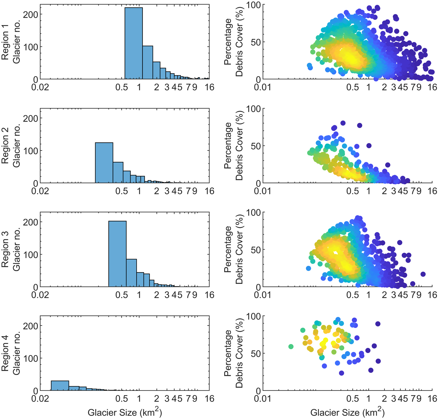
Fig. 6. Description of glacier number by glacier area and plots of percentage debris-covered ice against glacier size for each geographical region show in Figure 1.
The median aspect ratio of glaciers at four sub glacier regions in Afghanistan was oriented towards the northeast and northwest (Fig. S8, Supplementary Material).
4.3 Drivers of debris cover based on PCA-based analysis
The initial attempt to identify controls on debris cover fractions considers the complete glacier database. The PCA identified five PCs that represented 72% of the original dataset (Table 5). Only components with significance loadings were included in the stepwise regression. The latter used percentage debris-covered ice as the dependent variable (Table 5) which had a resultant R 2 of 43.7%.
Table 5. Loadings of each original variables (all dataset) on each principal component with more than 5% contribution to the variance of the original data. Important variables are flagged in bold (correlations >0.7 or <−0.7)

Note: Data in bold typeface are identified with correlations >0.7 or <−0.7. (/) indicates variable is not entered into the stepwise regression.
There are six variables that contribute to the PCs (Table 5) and each PC is then labeled based on these contributions (Table 6). The first most important component identified in the regression was PC2 which is associated with variables that describe glacier length and elevation range. It explained 19.1% of the original data and was negatively associated with percentage debris cover. Thus, larger glaciers with greater elevation ranges tend to have lower percentage debris-covered ice. The second most important component ranked was PC4, which represented glacier width and which explained 12% of total variability in original data (Table 6). This suggests that wider glaciers have lower percentage debris-covered ice. The third most important component ranked was PC3, which represented glacier/catchment slope parameters and which explained 16% of the total variability in the original data (Table 6). The sign of association suggests that steeper glaciers are more prone to higher percentage debris-covered ice. PC1 that corresponds to catchment size explained 22% of total variability in the original data but was not included in the stepwise regression.
Table 6. PCA results based on the complete dataset

Rows are sorted vertically by importance of contribution to the stepwise regression model. N indicates no PC identified with this interpretation. / indicates not added to the stepwise regression.
Given the possibility of strong spatial dependence in these analyses associated with broad-scale regional controls (e.g. climate, geology), it is possible that analysis of the entire dataset masks underlying drivers of debris cover. Thus, we undertook the same analysis but by climate zone and geological region. The Tables S2 and S3 in Supplementary Material contain the full results and we only present summary tables here.
A consistency and coherence in terms of the sign of the association of individual PCs and debris cover was found in general for all datasets whether classified by climate or geology; although there were some differences, such as in the details of the variables that contributed to each component.
For all climate zones, the PC that is associated with glacier length and elevation range is ranked as the most or second most important component (Table 7). PCs associated with glacier width are ranked as the second or third most important component. They are negatively associated with percentage debris cover through all climate zones and suggest that longer and wider glaciers have less debris-covered ice. Glacier altitude is ranked as the most important in climate zones 2 and 4 and the fourth most important component in climate zone 1, but is not significant in zones 3 and 5. Glacier altitude is negatively associated with percentage debris cover, suggesting higher altitude glaciers have proportionately less debris-covered ice. The glacier/catchment slope component is positively associated with debris cover in all climate zones, ranked as the second most important component in zone 3, the third most important component in zones 1, 4 and 5 and the fourth in zone 2. The sign suggests that steeper ice and catchment slopes lead to greater percentage debris cover. Catchment size in zones 2, 3 and 4 was not included in the stepwise regression. However in zone 1 it was ranked the fifth most important component with a positive association; and in zone 5 it was ranked as the fourth most important component with a negative association. The positive sign of association suggests that bigger catchment areas have higher percentage debris cover. However, the negative sign of association may be due to the fact that catchment size is also related to glacier length, width and elevation range parameters. This indicates that longer and wider glaciers are associated with larger catchments, and therefore negatively associated with percentage debris-covered ice.
Table 7. PCA results based on climatic zone classifications

C Z1: Climate zone 1 (Arid, desert, cold).
C Z2: Climate zone 2 (Arid, steppe, cold).
C Z3: Climate zone 3 (Cold, dry summer, hot summer).
C Z4: Climate zone 4 (Cold, dry summer, hot summer, Monsoonal Influence).
C Z5: Climate zone 5 (Temperate, dry summer, hot summer).
N indicates no PC identified with this interpretation. / indicates not added to the stepwise regression.
Table 8 shows the results when glaciers are classified into the six geological categories. This classification leads to higher levels of explanation (R 2) for some classes as compared with modeling using the full dataset or divided into climatic zones. It suggests that the assumed linear ranking of resistance to erosion used for the full dataset does not represent geological effects well and that once divided into geological zones, geological controls on debris production are represented more effectively. As with the significant majority of the preceding analyses the principal component that represents glacier length and elevation range is ranked as the first most important in zones 2, 3, 5 and also first but combined with catchment size in zone 6. It is ranked the second most important in zones 1 and 4. The associations with debris cover remain negative. The component representing the glacier width ranked the most important in zone 1 and second in zones 2 and 3, whereas it combined with the variables glacier length and elevation range for other zones and with negative associations.
Table 8. PCA results based on glacier geological zones
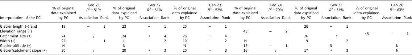
Geo Z1: Geological zone 1 (Chemical organic).
Geo Z2: Geological zone 2 (Detrital sedimentary).
Geo Z3: Geological zone 3 (Igneous).
Geo Z4: Geological zone 4 (Igneous and detrital sedimentary).
Geo Z5: Geological zone 5 (Metamorphic).
Geo Z6: Geological zone 6 (Metamorphic and igneous).
N indicates no PC identified with this interpretation. / indicates not added to the stepwise regression.
Components representing catchment size were the fourth most important in zones 2 and 3. In zone 4 the debris influence area in the catchment was ranked as the third most important component. In these three cases there was positive association. In zone 6 and zone 4 (catchment area only) combined with glacier length, width and elevation range and there were negative association signs. These indicate that glaciers with bigger debris influence areas also tend to have higher percentage ice-covered debris while larger catchments do not necessarily have bigger debris influence areas and are more influenced by glacier length, width and elevation range. The principal component that represents variables relating to glacier/catchment slope is ranked third in geological zones 2, 3 and 5 but is not identified for other zones. The positive association with debris cover suggests that glaciers, and their catchments, with steeper slopes tend to have higher percentage ice-covered debris in certain geological zones. The principal component associated with glacier altitude appears only for geological zone 4, and is the most important component and with a negative sign of association.
5. Discussion
5.1 Indices of glacier debris cover
Glaciers in the Himalaya are commonly associated with debris-laden ice avalanches and rockfall onto glacier surfaces from steep surrounding slopes (Shroder and others, Reference Shroder, Bishop, Copland and Sloan2000; Kaushik and others, Reference Kaushik, Joshi and Singh2019). Thus, mapping glacier extent and its change through time needs to take into account debris-covered ice. Paul and others (Reference Paul2015) have reported that errors involved in mapping glaciers can be significant when glaciers are heavily debris-covered and that this is a major challenge for glaciological studies (Shukla and others, Reference Shukla, Arora and Gupta2010; Paul and others, Reference Paul2015). The complex physical characteristics of debris-covered ice make it difficult to map with optical remote sensing (Holobâcă and others, Reference Holobâcă2021). Most studies are limited to small geographical regions and where only a small number of glaciers (<5) are analyzed (Robson and others, Reference Robson2015; Kaushik and others, Reference Kaushik, Joshi and Singh2019). Inventories also exist with more specific region-based calibration but these have tended to focus on glaciers >1 km2 in size (e.g. Scherler and others, Reference Scherler, Wulf and Gorelick2018; Herreid and Pellicciotti, Reference Herreid and Pellicciotti2020; Fleischer and others, Reference Fleischer, Otto, Junker and Hölbling2021). In this study, a combination of two thermal indices showed encouraging results for remote sensing of debris-covered ice over a spatially extensive zone. While Lougeay (Reference Lougeay1974) argued that thicker layers of debris may weaken TIR signals, field data for the Mir Samir Glacier clearly show that signals could be captured under thicker debris cover, even if the maximum depth that can be measured was not established in this study. It emphasizes the value of continued research with thermal infrared data and necessary downscaling methods.
As is standard practice, our NIR and SWIR datasets were corrected for top of the atmosphere effects. However, such correction introduced more noise into the thermal based debris cover index and coarsened the resolution of the outputs (Fig. S5, Supplementary Materials). Thus, we did not correct the thermal band used in (1) for TOA effects. We can justify the lack of correction in three ways. First, we note that converting TIR DNs to TOA is a linear correction process that should not make much difference and which is also undertaken because it is dependent on local meteorological data that are themselves highly uncertain especially in remote regions (USGS, 2022). Second, using non atmospheric corrected imagery at high altitudes appears to have minimal influences on mapping (Bishop and others, Reference Bishop2000) and other researchers have obtained better results and transferability using DNs for mapping glaciers (Bhambri and others, Reference Bhambri, Bolch and Chaujar2011; Haireti and others, Reference Haireti, Tateishi, Alsaaideh and Gharechelou2016). Third, we undertook checks by comparing the DN-TOA relationships for different images (Supplementary Material). These showed very little variation in the range of ToA values used for image thresholding, suggesting our index is likely less sensitive to ToA variations and the index thresholds should be transferable. By extending validation to multiple glaciers within Afghanistan and beyond might require ToA correction due to use of images obtained at different times/dates. However, even without ToA correction we did not find a clear pattern of degradation in accuracy statistics (Table 3), and the threshold for identifying debris-covered ice seemed to transfer without further calibration. We nonetheless suggest that this conclusion is checked if this index is applied elsewhere.
Most of the TIR signals suggesting debris-covered ice were associated with igneous rocks (mainly granite and granodiorite) less prone to weathering and leading to coarser and likely drier surface debris. In our case, we identified a second situation where the TIR signal was absent but it was clear that there was debris-covered ice. The second index (2) was crucial for glaciers whose geology was associated with detrital sedimentary rocks, more readily weathered and leading to smaller grain-sizes and a wetter surface. This is an important finding for debris-covered ice mapping from remote sensing, but one that needs further testing.
As with other studies (e.g. Herreid, Reference Herreid2021; Stewart and others, Reference Stewart2021), the real challenge with developing new indices such as ours is obtaining data for calibration and/or validation and calibration suggested that the classification thresholds were important. We found that using a relatively low threshold for the debris cover indices increased the commission error, but using a relatively high threshold increased the omission error (Wang and others, Reference Wang, Gao, Zhang, Wang and Yang2020). Therefore, selecting an optimal threshold is still a challenging task. A weakness of this study is having field observations from only one glacier; but the remoteness of glaciers in Afghanistan combined with on-going security problems makes this a challenge. That said, the transferability of the threshold we optimized from field-based calibration to other glaciers (Table 3) is reassuring.
The combination of TIR with panchromatic imagery was central to allowing us to map glaciers much smaller than those typically mapped by others using remote sensing. For instance, Herreid and Pellicciotti (Reference Herreid and Pellicciotti2020) set a minimum glacier size as 1 km2 and Scherler and others (Reference Scherler, Wulf and Gorelick2018) obtained poorer mapping accuracies for glaciers less than 1 km2. Figure 6 shows that Afghanistan's glaciers are mainly smaller than 1 km2. Figure 3 also shows that our indices produce greater extents of debris-covered ice than in published inventories. The presence of crevasses and ponds in these zones confirms that these enlarged zones are indeed ice-cored. The zones tend to be somewhat irregular and also contain holes, commonly where glacier retreat has left exposed bedrock patches, rather than debris-covered ice. This corresponds to the fact that debris-covered ice in High Mountain Asia tends to have a complex morphology and hummocky, rugged topography (Miles and others, Reference Miles2020).
The identification of more extensive zones of debris-covered ice in our index largely explains why our accuracy statistics are better (Table 3) but these also emphasize a key point. Our goal was to map debris-covered ice, and not simply debris-cover on glaciers. Rapid glacier retreat is likely leading to extensive debris-covered ice that may become progressively disconnected from the glacier. Whether such zones are included as ‘glacier’ or not is a debatable point. In our case, with a long-term goal of understanding glacier retreat for Afghan water resources, our interest is in debris-covered ice whether or not it remains connected to the glaciers. Thus, we do not argue that our approach is better, rather that it is more appropriate if the scientific goal is mapping debris-covered ice rather than debris cover on glaciers.
5.2 The glacier inventory
We identified 3408 glaciers (⩾0.01 km2) covering 2,841 ± 51.1 km2 in area using datasets for 2016. Maharjan and others (Reference Maharjan2018) identified 3782 glaciers (⩾0.01 km2) with 2539 km2 of area for 2015. One year is not enough for these differences to be real and we think that they arise because Maharjan and others (Reference Maharjan2018) used the normalized difference snow index (NDSI) for glacier mapping and a single slope threshold for mapping debris-covered ice. The larger number of glaciers then relates to the fact that they considered glaciers with size ⩾ 0.01 km2; and underestimation of glacier area corresponds to the fact that the NDSI could not detect zones of glaciers under shadow as well as ice covered by thicker debris. In addition, the slope threshold of <24°, used by Maharjan and others (Reference Maharjan2018), may not detect debris cover when the glacier tongue transition to the unglaciated zone is gentle (Paul, Reference Paul2003; Bolch and Kamp, Reference Bolch and Kamp2005; Frey and others, Reference Frey, Paul and Strozzi2012).
This study estimated 619 ± 40 km2 of debris-covered ice for Afghanistan and a total debris cover as a percentage of glacier area of ~ 22%. This is higher than for south-west Asia as a whole (Herreid and Pellicciotti, Reference Herreid and Pellicciotti2020) but it also masks substantial within-region variation (Table 4) of between 8 and 42% debris cover. It also reflects the fact that we consider debris-covered ice and not just debris-covered glacier.
5.3 Controls on debris cover
Assessment of debris-cover development on Afghan glaciers by principal component analysis showed that considering all glaciers in a single analysis masked sensitivity to certain drivers. Dividing the dataset into two classes based on climate zones and geological zones produced more clear findings. Components that represented variables related to glacier length, width and elevation range were uniformly found to be highly important, with bigger glaciers (in terms of length/width) inevitably having a higher range and less debris-covered ice.
Components associated with glacier mean altitude were only found to be important for certain climate zones, notably zones 2 and 5 (Table 7), for geological zone 4 (Table 8). The importance of altitude no doubt reflects the fact that the lower glaciers are more ablation prone and so more prone to accumulating debris, as others observed (e.g. Fleischer and others, Reference Fleischer, Otto, Junker and Hölbling2021). However, the relative lack of importance of altitude-related as compared with size-related components, and the relatively low correlation of altitude with width (r = 0.281) and length (r = 0.233) emphasizes that altitude is not a primary driver of the extent of debris cover in Afghanistan.
Geology was rarely correlated with significant PCs for the full dataset. However, separating by geological zones resulted in sets of PCs that explained higher proportions of debris cover (Table 8) and clearer and consistent results across zones in terms of the association between components their most correlated variables and debris cover. Few studies have investigated lithological controls on rockfalls and glacier debris cover at regional scales, and data are usually not available for larger areas (Marquinez and others, Reference Marquinez, Duarte, Farias and Sanchez2003; Messenzehl and others, Reference Messenzehl, Meyer, Otto, Hoffmann and Dikau2017; Fleischer and others, Reference Fleischer, Otto, Junker and Hölbling2021). Geological drivers of differences in debris-cover development on glaciers merit further work.
Globally, the relative percentage of debris cover areas systematically decreases from 14% to 0% as glacier size increases although this pattern is not the same for all the regions (Scherler and others, Reference Scherler, Wulf and Gorelick2018). We found a similar association, albeit with a higher percentage debris cover variation (between 0 and 80%) (Fig. 6). Huang and others (Reference Huang, Li, Zhou and Zhang2021) suggested a latitudinal variation with the regional percentage of debris cover a negative exponential function of distance from the equator, implying that warmer climatic zones are more dynamic and conducive to supraglacial debris production. However, orographic factors such as mountain-range, age, relief and lithology may cause regional-scale exceptions to this relation (Herreid and Pellicciotti, Reference Herreid and Pellicciotti2020).
Chowdhury and others (Reference Chowdhury, Sharma, Kumar and Debnath2021) observed that a relatively gentle slope with lower elevations in ablation areas could be favorable for the abundant accumulation of supraglacial debris. However, for all climate zones and geological zones (Tables 7 and 8) while it is clear that low slopes encourage debris accumulation, our results suggest that steep slopes can also lead to high debris cover likely because of their impacts on sediment production.
6. Conclusion
Using field observations and manual glacier maps, we developed two new indices to map glaciers and debris-covered ice in Afghanistan with promising results. During the mapping process, we were able to distinguish between different debris-covered ice in terms of their geological formations and thermal characteristics. The result of the mapping was a new glacier inventory for Afghanistan. Our analysis, based on 3408 glaciers, showed that Afghan glaciers are highly debris-covered, at 21.7 ± 1.4% of total glacier area, although this varies regionally; regions with smaller glaciers tend to have higher percentage debris cover. The characteristics of glaciers in Afghanistan, and their debris cover, are dependent on climate and geology. Debris cover is predominantly affected by measures of glacier length, width and elevation range; higher values of these measures tend to be associated with glaciers with less debris cover. Catchment size effects are complex and vary by region. The proportion of non glacier area in a catchment appears to an important influence on debris cover development. Drier climates tend to produce higher debris cover as do glaciers in geological zones with more readily-weathered sediment.
Supplementary material
The supplementary material for this article can be found at https://doi.org/10.1017/jog.2023.14.
Acknowledgements
We greatly appreciate and thank Afghanistan government offices that supported this research, special thanks to the Ministry of Energy and Water (MEW) of Afghanistan for facilitating our fieldwork, Ministry of Mines and Petroleum of Afghanistan and Ministry of Agriculture Irrigation and Livestock of Afghanistan for providing us high-resolution spatial datasets. We acknowledge and appreciate Prof. Horst Machguth's contribution for calculating the glacier length for our dataset with his method. This research was supported by Swiss Government Excellence Scholarship Program, we thank them for their continued support. We finally would like to thank three anonymous reviewers and the Scientific Editor Prof. Joseph Shea for having contributed to the improvement of the manuscript.


 Open access