


1. INTRODUCTION
Ice shelves play an important role in inhibiting sea-level rise as they buttress glaciers on land and restrain ice discharge to the circum-Antarctica seas that merge with the Southern Ocean (MacAyeal, Reference MacAyeal, Van der Veen and Oerlemans1987; Rignot and others, Reference Rignot2004; Scambos and others, Reference Scambos, Bohlander, Shuman and Skvarca2004). Volume loss of Antarctic ice shelves (Paolo and others, Reference Paolo, Fricker and Padman2015) reduces buttressing, which raises concerns of consequent acceleration of glacier discharge, raising sea level. Ice shelf volume loss results from ice shelf thinning due to enhanced ocean-driven melting and iceberg calving (Pritchard and others, Reference Pritchard2012; Paolo and others, Reference Paolo, Fricker and Padman2015). Numerical modeling (Sergienko, Reference Sergienko2010; Lipovsky, Reference Lipovsky2018) and observations (MacAyeal and others, Reference MacAyeal2006; Brunt and others, Reference Brunt, Okal and MacAyeal2011) indicate that ocean gravity wave impacts can expand existing crevasses and fractures, leading to calving events and/or contributing to a reduction of ice shelf integrity. Seasonal loss of sea-ice leaves the outer ice shelf margin directly impacted by swell, which may have contributed to the collapse of the Larsen A and B and Wilkins ice shelves (Massom and others, Reference Massom2018). However, modeling suggests that swell alone may not provide sufficient forcing to induce ice shelf disruption (Lipovsky, Reference Lipovsky2018).
Considering the persistent strong Southern Ocean storm activity and the associated intense ocean wave climate that continuously impacts ice shelves (Trenberth, Reference Trenberth1991; Tolman, Reference Tolman2009; Chapman and others, Reference Chapman, Hogg, Kiss and Rintoul2015), ocean wave impacts likely play a role in ice shelf evolution. Thus, it is important to quantify the spatial and temporal response of ice shelves to ocean gravity waves with in-situ measurements. This will improve modeling of ice shelf/ice-sheet response to climate change and consequently reduce the uncertainty in ice-sheet mass loss projections over the coming decades.
To better understand the response of ice shelves to ocean-gravity-wave impacts, we deployed a broadband seismic array on the Ross Ice Shelf (RIS) from October 2014 to November 2016 (Bromirski and others, Reference Bromirski2015; Diez and others, Reference Diez2016). The seismic network consisted of two linear transects in a cross-like configuration that were approximately parallel and orthogonal to the shelf front (Fig. 1a) and included a dense subarray at the intersection of the two transects. Station separations within the transects were typically 80–90 km, while separations in the center subarray were ~5–10 km. The large array aperture and multi-year deployment allowed the spatial, seasonal and interannual variations of the ice shelf response to ocean forcing to be quantified and provided baseline observations to identify the magnitude of change in future studies.
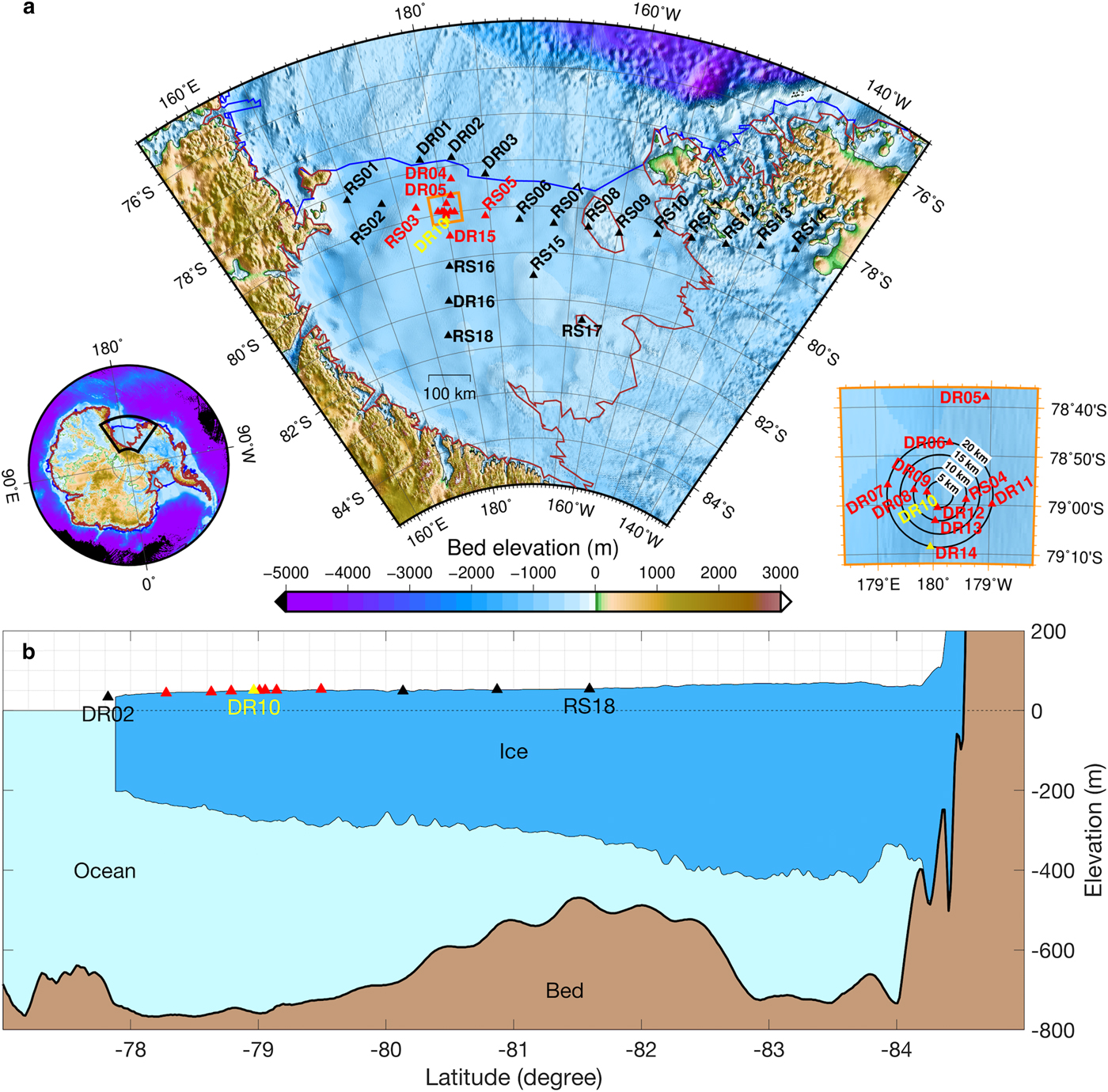
Fig. 1. (a) The RIS seismic stations (triangles) superimposed on the bed elevation map (Fretwell and others, Reference Fretwell2013), with the center station DR10 (yellow), extended center subarray (red) and other stations (black) indicated. The RIS is bounded by the grounding line (brown line) and the ice front (blue line). An expanded view of the dense center subarray (orange box) is shown in the right inset, where the contours of distance to DR10 are shown (black circles). (b) Cross-section along the 180° meridian (Fretwell and others, Reference Fretwell2013). DR02 is off the ice front because the ice front has moved northward, but the ice thickness model has not been updated.
In addition to the RIS array, data from a 5-station broadband seismic array deployed on the Pine Island Glacier (PIG) ice shelf from January 2012 to December 2013 (Christianson and others, Reference Christianson2016) were used for comparative analyses. This seismic array was ~20 km from the PIG front, with station separation ~2 km. These data allow comparison of the response of a large ‘stable’ ice shelf (the RIS) to the much smaller less ‘stable’ PIG ice shelf. There are significant differences in size, ice flow speed and thinning rate of RIS and PIG. Seismic comparisons between the two shelves will show whether they have a different response to gravity-wave forcing, which can be used to estimate and compare their properties. The smaller station separation of the PIG array presented the possibility of detecting higher-frequency shorter wavelength signals than the RIS array. However, the few stations and a small aperture of the PIG array preclude a detailed comparison with the RIS array results.
In this paper, we first introduce the geometry of the RIS and the PIG ice shelf. Then we introduce plate wave theory and discuss the generation mechanism. A swell event impacting the RIS during austral summer when sea ice was absent is then analyzed from both observational and theoretical perspectives. Beamforming and cross-correlation techniques are employed to obtain the signal propagation direction and the dispersion relation, which indicate the wave types and ice shelf elastic properties. Principal component analysis quantifies particle motion characteristics, which assist in the identification of the wave types. Finally, plate waves observed on the PIG ice shelf are discussed and compared with RIS observations.
2. STUDY REGIONS
2.1. RIS
RIS ice thicknesses are 240–340 m at the ice front, and increase up to 700–800 m near the grounding zone (Fretwell and others, Reference Fretwell2013). The geometry of a cross-section roughly along the north-south array transect shows the variation of the ice thickness and the bathymetry (Fig. 1b). Along the cross-section, the ice thickness is ~240 m at the ice front and gradually increases to ~330 m under DR10 (the center of the dense subarray, ~130 km from ice-front station DR02). Under RS18 (the southern most station, ~380 km from the ice front), the ice thickness is ~370 m. The seafloor depth varies between 600 and 800 m near the ice front, with the sub-shelf water thickness decreasing from ~500 m near the ice front to ~480 m below DR10 and ~160 m below RS18, which sits above a basement high.
2.2. PIG ice shelf
The PIG ice shelf (~3000 km2, Bindschadler and others, Reference Bindschadler, Vaughan and Vornberger2011) is much smaller than the RIS (472 960 km2, Scambos and others, Reference Scambos, Haran, Fahnestock, Painter and Bohlander2007). However, it is the largest regional contributor to sea-level rise (Medley and others, Reference Medley2014). The ice flow speed near the ice shelf front increased from ~2.3 km a−1 to ~4.0 km a−1 from 1974 to 2008 (Joughin and others, Reference Joughin, Rignot, Rosanova, Lucchitta and Bohlander2003, Reference Joughin, Smith and Holland2010), while the ice flow speed at the RIS is generally <1.2 km a−1. The increased flow rate at the PIG ice shelf suggests that it is less stable than RIS. In contrast to RIS, rapid melting occurs beneath the PIG ice shelf due to the warm Circumpolar Deep Water (CDW) intruding the Amundsen Sea coast (Jacobs and others, Reference Jacobs, Hellmer and Jenkins1996; Thoma and others, Reference Thoma, Jenkins, Holland and Jacobs2008; Joughin and others, Reference Joughin, Smith and Holland2010; Bindschadler and others, Reference Bindschadler, Vaughan and Vornberger2011), with enhanced thinning potentially weakening PIG.
The PIG ice shelf is over 1 km thick at its grounding line and thins to ~300 m at the ice front (Bindschadler and others, Reference Bindschadler, Vaughan and Vornberger2011). The average thicknesses of the PIG seismic array sector (~460 m) and the RIS beamformed subarray sector (~300 m) are comparable. The water layer thickness at the PIG ice front is ~500 m and decreases to ~200 m over a distance of 35–40 km away from the ice front (Bindschadler and others, Reference Bindschadler, Vaughan and Vornberger2011). There are no bathymetry data more than 40 km inland from the shelf front.
3. PLATE WAVE THEORY
Ice shelves can be viewed as floating plates of ice formed by glacier outflows. Ocean surface gravity waves impact ice shelves, couple wave energy with the ice and excite seismic plate waves. Propagation characteristics of gravity-wave-excited plate waves provide information on the elastic properties of the ice, which can be related to ice shelf integrity, i.e. weaker, more fractured ice (PIG) will behave differently than more competent (RIS) ice.
There are three types of ocean surface gravity waves below 100 mHz that excite plate waves in ice shelves: (1) very-long-period (VLP) gravity waves (<3 mHz): tsunami and meteorologically-forced waves, (2) infragravity (IG) waves (3–20 mHz), generated by nonlinear wave interactions along coastlines (Herbers and others, Reference Herbers, Elgar and Guza1995; Bromirski and others, Reference Bromirski, Sergienko and MacAyeal2010) and under mid-ocean storms (Uchiyama and McWilliams, Reference Uchiyama and McWilliams2008) and (3) swell (30–100 mHz), generated by cyclonic storm systems where wind energy couples into ocean swell. At lower frequencies (<20 mHz for the RIS), gravity provides a restoring force that is significant in ocean/ice shelf coupling, generating flexural-gravity waves (Fox and Squire, Reference Fox and Squire1990). At higher frequencies (>20 mHz for the RIS), where the gravity restoring force is negligible, Lamb waves, with both symmetric (extensional) and anti-symmetric (flexural) modes, are excited (Lamb, Reference Lamb1917).
3.1. Lamb waves
3.1.1. Dispersion relation
Lamb waves have multiple modes, described by the dispersion relations first developed by Rayleigh (Reference Rayleigh1888) and Lamb (Reference Lamb1889), with a more systematic analysis by Lamb (Reference Lamb1917). To implement the system of equations, we construct a 3-dimensional x-y-z coordinate system, with the horizontal x−y plane coinciding with an infinite-extent ice plate of 2 h-thickness. This coordinate system assumes that plane waves propagate in the x direction with plane strain in the y direction. Let k P, k S and k L be the wavenumbers of the P wave, S wave and Lamb waves, respectively. For stress-free boundaries, the frequency equations are obtained as modified from Graff (Reference Graff1991),
 $$\displaystyle{{\tanh k_2h} \over {\tanh k_1h}} = \left[ {\displaystyle{{4k_1k_2k_L^2 } \over {{(k_L^2 + k_2^2 )}^2}}} \right]^{ \pm 1},$$
where k 1 and k 2 are defined as
 $$\eqalign{& k_1^2 = k_L^2 - k_P^2 , \cr & k_2^2 = k_L^2 - k_S^2 .} $$
The superscript on the right-hand side of Eqn (1) corresponds to symmetric (extensional) mode (+ 1) or anti-symmetric (flexural) mode (−1), identified by the particle motion symmetry with respect to the mid-plane of the plate.
The dispersion relation, i.e. Eqn (1), is numerically solved. Dispersion curves for both symmetric and anti-symmetric modes (Fig. 2a) have multiple higher-frequency sub-modes that depend on the vertical wavelength, represented by S n and A n for nth-order symmetric and anti-symmetric mode, respectively. These modes approach the Rayleigh wave speed (~0.92c S, where c S is S-wave speed) asymptotically at the high-frequency end. Only the very low-frequency end of the curves (k Sh < 0.12) applies to the response of the RIS (Fig. 2b). Specifically, Lamb waves are observed below 100 mHz with array methods, above which the coherence between stations drops to an unobservable level due to a combination of higher attenuation, and/or lower source power and/or seismic station spacing. In addition, the ice shelf thickness 2 h is <620 m over the seismic array (except land stations) (Fig. 1b). Assuming the S-wave speed of glacial ice c S = 1.58 km s−1 (Table 1), at frequencies f < 100 mHz, we have
 $$k_Sh = \displaystyle{{2\pi f} \over {c_S}}h < \displaystyle{{2\pi \times 100\;{\rm mHz}} \over {1.58\;{\rm km}{\mkern 1mu} {\rm s}^{ - 1}}} \times \displaystyle{{620\;{\rm m}} \over 2} \approx 0.12,$$
which indicates that only fundamental symmetric and anti-symmetric modes (S 0 and A 0) are observable on the RIS (Fig. 2a). Theoretical free-space Lamb wave dispersion curves (Fig. 2b) of a vacuum-ice-vacuum (VIV) model (Fig. 3) are given as a rough approximation for the RIS.
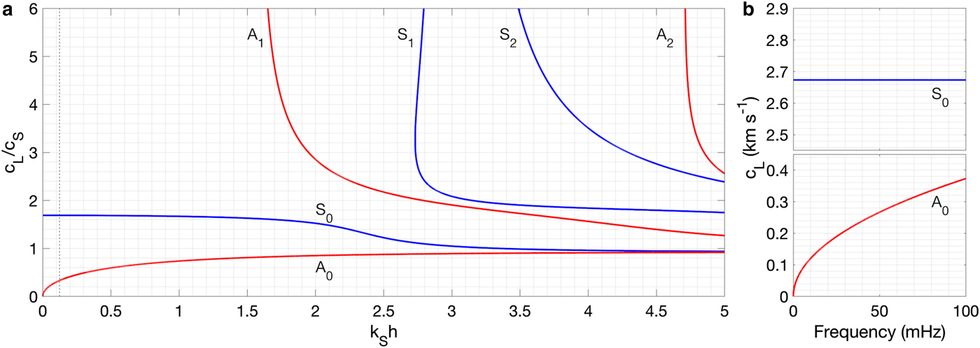
Fig. 2. (a) Dispersions curves of free-space Lamb waves for Poisson's ratio ν = 0.3. The horizontal axis is the product of the S-wave wavenumber k S and the half plate thickness h, with the vertical axis the Lamb-wave phase speed c L normalized by S-wave speed c S. The low-frequency part of the curves (k Sh < 0.12, left of the black dashed line) resulting from low-frequency gravity-wave forcing applies to the RIS observations. (b) Dispersion curves of free-space Lamb waves in the vacuum-ice-vacuum (VIV) model (see Fig. 3).
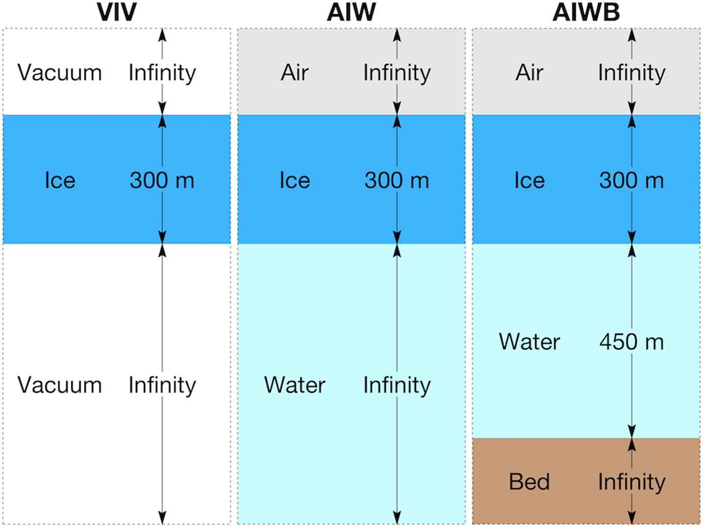
Fig. 3. Model geometry for vacuum-ice-vacuum (VIV), air-ice-water (AIW), and air-ice-water-bed (AIWB) cases. The layer properties are given in Table 1.
Table 1. Model parameters. The parameters c P, c S, and ρ denote the P-wave speed, S-wave speed and density of each layer. Parameters for air are for dry air at 15 °C at sea level. The c P and c S values of (intact) ice are calculated from Young's modulus E = 6 GPa and Poisson's ratio ν = 0.3. Parameters for water are the approximate values for sea water. The bed properties for modeling  $S_0^\ast $ and $A_0^\ast $ with OASES are those of the uppermost solid layer of PREM (Dziewonski and Anderson, Reference Dziewonski and Anderson1981). The bed is assumed rigid to obtain a simpler analytical solution of flexural-gravity waves (Fox and Squire, Reference Fox and Squire1990)

3.1.2. Particle motion
For Lamb waves under stress-free boundary conditions, or free-space Lamb waves, the horizontal (U) and vertical (W) particle motions of S 0 and A 0 modes are determined from the modified solutions of Viktorov (Reference Viktorov1967, Eqn (II.21) and (II.22)) as
 $$\eqalign{& U_{S_0} = Ak_S\displaystyle{{k_{LS_0}^2 - k_2^2 } \over {k_{LS_0}^2 + k_2^2 }}\displaystyle{1 \over {k_Sh}}\sin (k_{LS_0}x - \omega t), \cr & W_{S_0} = Ak_S\displaystyle{{k_{LS_0}^2 - k_2^2 } \over {k_{LS_0}^2 + k_2^2 }}\displaystyle{{k_1z} \over {k_Sh}}\cos (k_{LS_0}x - \omega t),} $$
and
 $$\eqalign{& U_{A_0} = Bk_S\displaystyle{{k_Sz} \over 2}\sin (k_{LA_0}x - \omega t), \cr & W_{A_0} = Bk_S\displaystyle{{k_S} \over {2k_{LA_0}}}\cos (k_{LA_0}x - \omega t),} $$
where  $k_{LS_0}$ and $k_{LA_0}$ are the wavenumbers of the fundamental S 0 and A 0 modes of the Lamb waves. The parameters A and B are constants that are determined by the particle motion amplitude, while ω is the angular frequency.
According to Eqns (4) and (5), for a thin plate (k Sh ≪ 1), horizontal displacements (extensional motions) are dominant for the S 0 mode, while vertical displacements (flexural motions) are dominant for the A 0 mode. In addition, the particle motions of S 0 and A 0 modes are both retrograde. But these retrograde motions are difficult to observe since the ellipticity is very high, and thus background noise may overwhelm displacements along the minor axis.
For ice shelves, where flexural motions of the ice are coupled to motions of the water layer, the dispersion curves are different from the free-space Lamb wave dispersion curves. The extensional motions of the RIS have small vertical displacements and are minimally affected by the ice-water coupling, thus should be close to the free-space S 0 mode, represented by  $S_0^\ast $. In contrast, the flexural motions in the RIS might be appreciably different than the free-space A 0 mode, represented by $A_0^\ast $. Synthetic modeling is necessary to assess the coupling effects on the flexural motions.
3.1.3. Synthetic modeling
To explore the effects of the components of the air-ice-water (AIW) system representative of seismic wave propagation on the RIS, synthetic seismograms were computed for VIV and AIW models (Fig. 3). The modeling was implemented using OASES, a seismo-acoustic package (Schmidt, Reference Schmidt2004), with ice properties given in Table 1. The source function is a Ricker wavelet centred at 50 mHz, representing 20 s period ocean swell impacting the RIS. Since we are dealing with long-wavelength seismic waves (>3 km), the small-scale structure should not have a significant effect on seismic wave propagation in the frequency bands studied. For example, the surface firn layer thickness is of the order of 50 m (Diez and others, Reference Diez2016), which will have minimal effect in the frequency bands investigated. However, as has been shown by variable ice shelf responses in observations (Bromirski and others, Reference Bromirski2017) and modeling (Sergienko, Reference Sergienko2017), ice shelf and sub-shelf water layer thicknesses can have a significant effect.
For the VIV model, non-dispersive fundamental extensional Lamb waves S 0 traveling at 2.67 km s−1 can be identified (Fig. 4a), consistent with the theoretical dispersion curve of the S 0 mode (Fig. 2b). The wave amplitude decreases with the range due to geometrical spreading. Fundamental flexural Lamb waves A 0 are highly dispersive near the 50 mHz source frequency selected (Fig. 4c), with phase speed of 0.27 km s−1 that is roughly consistent with the theoretical value for the A 0 mode (Fig. 2a).
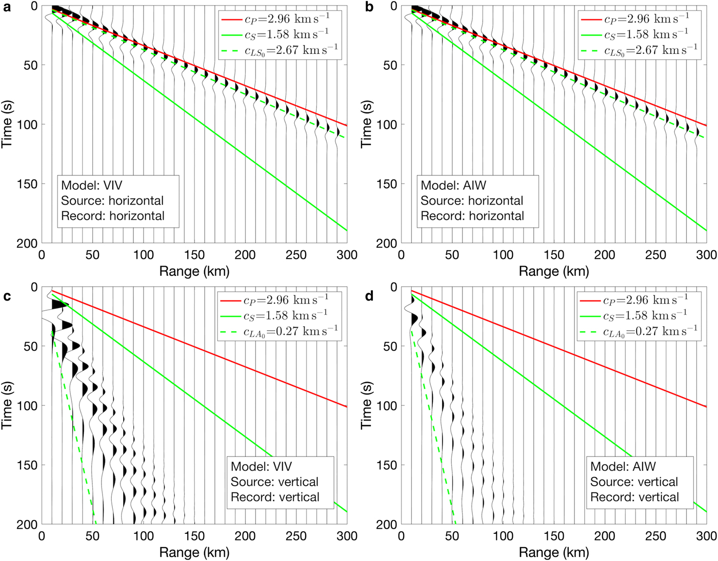
Fig. 4. Synthetic seismograms of the (a,b) horizontal (radial) component and (c,d) vertical component on the ice layer surface in model VIV (a,c) and AIW (b,d). The source function is a Ricker wavelet centered at 50 mHz, with a horizontal point force in (a,b) and vertical point force in (c,d). The normalizations for horizontal motions in (c) and (d) are 10 times those of (a) and (b). P-wave speed (c P, red solid), S-wave speed (c S, green solid) and fundamental free-space Lamb-wave phase speeds ( $c_{LS_0}$ and $c_{LA_0}$, green dashed) at 50 mHz are indicated.
For the AIW model, the extensional Lamb waves,  $S_0^\ast $, are observed for the AIW model with the same phase and group speeds and similar attenuation as S 0 for VIV (Fig. 4a,b; green dashed lines), showing that the water layer has little effect on extensional motions. The flexural Lamb waves, $A_0^\ast $, are observed for AIW but have lower amplitude than A 0 for VIV due to energy coupled into the water layer (Fig. 4c,d). The phase speed of $A_0^\ast $ cannot be identified due to dispersion and low amplitude.
3.2. Flexural-gravity waves and Flexural waves
At lower frequencies (<20 mHz), the gravity restoring-force effect is non-negligible, making it an inappropriate problem for OASES, as the effect of gravity is not included in OASES. However, an analytical solution for low-frequency flexural motions can be obtained by assuming a rigid bed below the water layer, i.e. the air-ice-water-bed (AIWB) model (Fig. 3), and a thin-plate model (plate thickness ≪ flexural-gravity-wave wavelength). Equations of the velocity potential field in water are constructed with ice-water boundary conditions on top and no vertical displacement at the bottom, yielding flexural-gravity waves excited at the ice/water interface. There are two traveling modes, four damped traveling modes and an infinite number of evanescent modes (Fox and Squire, Reference Fox and Squire1991). Traveling modes can be extracted by array coherence analysis. Because of the rapid attenuation of damped and evanescent modes with distance from the ice front, these modes contribute to relatively stronger vibrations only at the ice front. Although evanescent modes do not propagate efficiently, they are important in gravity-wave energy reflection and transmission. At higher frequencies (>20 mHz), the gravity restoring-force effect vanishes and the flexural-gravity-wave phase speeds approach flexural Lamb wave ( $A_0^\ast $) speeds, making them indistinguishable in this band. To differentiate these higher-frequency flexural motions from those where the effect of gravity is important, we term them flexural waves.
3.3. Dispersion comparison
To understand propagation characteristics of plate waves generated by ocean wave impacts at the RIS, we compared theoretical dispersion curves of A 0 for the VIV model, flexural waves, flexural-gravity waves and ocean surface gravity waves for the AIWB model (Fig. 5a) prior to determining the wave types from dispersion curves obtained with array processing of the observations. Note that the bed is assumed rigid for flexural-gravity waves and ocean surface gravity waves to simplify analytical solution, but is non-rigid when modeling flexural waves using crustal properties of the uppermost solid layer in PREM (Dziewonski and Anderson, Reference Dziewonski and Anderson1981). For flexural-gravity waves, the ice thickness of the RIS (mostly 200 to 400 m) is much smaller than plate-wave wavelengths (>3000 m) for frequencies below 100 mHz. Thus the thin-plate assumption is valid.
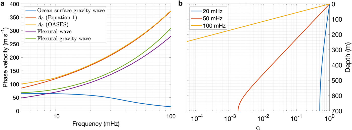
Fig. 5. (a) Dispersion curve comparison. The A 0 dispersion curve for the free-space ice plate in the VIV model is calculated by solving Eqn (1) (red), and by numerical modeling using OASES (yellow). The flexural wave dispersion curve of the floating ice plate in the AIWB model (purple) is calculated from numerical modeling with OASES. The dispersion curves from OASES modeling are smoothed using a moving average 15 mHz window. The thin-plate flexural-gravity-wave dispersion curve of the floating ice plate in the AIWB model (green) is based on Fox and Squire (Reference Fox and Squire1990). The ocean-surface-gravity-wave dispersion curve (blue) of a water layer of 450 m depth is given for reference. (b) The ratio between gravity-wave pressure perturbation amplitude at depth z and at the surface, or α(z), in a water layer of depth H = 700 m, according to Eqn (6).
The dispersion curve of A 0 in VIV calculated by OASES coincides with the analytical solution (Viktorov, Reference Viktorov1967) above 5 mHz, indicating good numerical stability except at very low frequencies. The  $A_0^\ast $ mode travels much slower in AIWB than A 0 does in VIV in the 10–100 mHz band, but closer to flexural-gravity wave speeds in AIWB, demonstrating the importance of water-layer coupling on plate-wave propagation. Below 10 mHz, the flexural-gravity-wave phase speed approaches the shallow-water gravity-wave phase speed (~70 m s−1), while the $A_0^\ast $ phase speed drops below the gravity-wave phase speed. This confirms that the gravity restoring-force effect is more significant at low frequencies. Hence, the flexural-gravity-wave formulation gives a better approximation of the flexural motions below 10 mHz than the $A_0^\ast $ dispersion.
3.4. Wave forcing mechanism
Excitation of flexural-gravity waves requires coupling of gravity-wave energy at the base of the ice shelf. Consequently, because pressure perturbations from surface gravity waves decrease exponentially with depth, ice shelf thickness is an important parameter in the coupling mechanism. The ratio between gravity-wave pressure perturbation amplitude at depth z and at surface is given by
 $$\alpha = \displaystyle{{\cosh [k_G(z + H)]} \over {\cosh (k_GH)}},$$
where H is total water depth (Kundu and others, Reference Kundu, Cohen and Dowling2011). The wavenumber k G at frequency f is determined by the gravity-wave dispersion relation
 $$c_G = \displaystyle{{2\pi f} \over {k_G}} = \sqrt {\displaystyle{g \over {k_G}}\tanh (k_GH)} ,$$
where c G is gravity-wave phase speed. The gravitational acceleration  $g=9.8\ {\rm m}\,{\rm s}^{-2}$. Combining Eqns (6) and (7), the relation between α and z is determined given H and f. Therefore, the geometry of the RIS is an important factor in determining the response ofthe gravity-wave forcing of the ice shelf.
The pressure perturbation decay curve at the RIS front (H ≈ 700 m) is determined at 20, 50 and 100 mHz (Fig. 5b). Lower-frequency gravity-wave pressure perturbations reach greater depths, illustrated by frequency-dependent α values at 206 m depth (base of the ice shelf front). At 50 mHz (corresponding to 20 s period swell), α = 0.13, only ~13% of pressure perturbation at 50 mHz signal reaching the base of the ice shelf front at 200 m depth. Furthermore, at 100 mHz, α = 2.5 × 10⁻⁴, resulting in little energy from wave-induced pressure perturbations above 100 mHz reaching the base of the ice shelf. In contrast, at 20 mHz, α = 0.73, indicating most of the low-frequency wave energy penetrates into the sub-shelf cavity. Pressure perturbations beneath the ice shelf couple with the ice and excite flexural-gravity waves.
Gravity-wave-induced pressure perturbations at the ice front can also excite extensional deformation. Since most of the wave energy below 20 mHz penetrates into the sub-shelf cavity, coupling with the ice shelf will occur at the ice/water interface. In contrast, because little higher-frequency (swell band) wave energy reaches the shelf base, energy exchange between swell and the ice shelf will occur primarily at the shelf front. Therefore, flexural-gravity waves and flexural waves are expected to be low-frequency dominant, while extensional Lamb waves are expected to be high-frequency dominant.
In summary, there are three wave types that are predicted to be observed at frequencies below 100 mHz:
(1) Extensional Lamb waves, $S_0^\ast $, are observed at higher frequencies (>20 mHz) and are generated by swell impacts at the ice shelf front.
(2) Flexural waves also observed at higher frequencies (> 20 mHz) where the gravity restoring force is weak, are generated by coupling of gravity-wave energy in the sub-shelf cavity with the ice shelf. Because the pressure from gravity waves decreases exponentially with depth, the wave energy penetrating the sub-shelf cavity is low at higher frequencies and the flexural-wave amplitudes are expected to be weak, if observable.
(3) Flexural-gravity waves, in the frequency band where the gravity restoring force has a significant effect, are generated by coupling of long-period gravity-wave energy in the ice-water system at the ice shelf base. These are expected to have greater amplitudes at lower frequencies (<20 mHz).

The 20 mHz cutoff is based on the RIS observations at the extended center subarray (Fig. 1a).
4. METHODS
4.1. Frequency-domain beamforming
Beamforming is an array processing method that combines elements of an array to reduce incoherent signals, utilizing constructive interference at particular azimuths and phase slownesses so that the azimuths and phase slownesses of coherent signals can be determined (Johnson and Dudgeon, Reference Johnson and Dudgeon1993; Van Trees, Reference Van Trees2002). The ice-shelf beamforming response depends on array geometry and signal wavelength. With the same station separation, a larger array aperture improves the slowness resolution if the signals at all stations are coherent.
The data matrix  $\bm {\bi d}$, for either vertical (Z), north (N), or east (E) component, is an m × n matrix, where m is the number of stations, while n is the number of data samples. For each azimuth θ to be checked, the horizontal components are transformed to radial (R) and transverse (T) directions with
 $$\eqalign{& {\bi d}_R = {\bi d}_N\cos \theta + {\bi d}_E\sin \theta \cr & {\bi d}_T = {\bi d}_N\sin \theta - {\bi d}_E\cos \theta ,} $$
where  $\bm {e}_i\ (i=N,\, E,\, R,\, T)$ represents the corresponding direction vector.
Let  $\bm {\bi D}$ be the element-wise phase of the Fourier transform of $\bm {\bi d}$. For each frequency bin centered at f, $\bm {\bi D}(f)$ is an m × 1 vector. The steering vector $\bm {\bi q}$ for a plane wave coming from the azimuth θ with wavenumber $\bm {\bi k}$, representing the phase delay at each station, is given by
 $${\bi q} = \left[ {\matrix{ {\exp ( - j{\bi k} \cdot {\bi r}_1)} \cr {\exp ( - j{\bi k} \cdot {\bi r}_2)} \cr \vdots \cr {\exp ( - j{\bi k} \cdot {\bi r}_m)} \cr } } \right],$$
where  $j = \sqrt {-1}$, while $\bm {r}_i$ is the position of the ith station. Then, the phase-only frequency-domain beamforming response is obtained by
 $$b = (\bm{\bi D}^H\bm{\bi q})^H\bm{\bi D}^H\bm{\bi q} = \bm{\bi q}^H\bm{\bi M}\bm{\bi q}, $$
where  $\bm {\bi M}=\bm {\bi D}\bm {\bi D}^H$; the superscript ‘H’ denotes the Hermitian.
For the RIS geometry, the ice-front source location is so close to the array that a large aperture makes the plane-wave assumption questionable. In addition, aliasing, the artifact in beamforming output is another array-geometry-related problem that affects beamforming quality. The main signal can be difficult to identify with beamforming at a particular frequency because of aliasing in the azimuth-slowness domain. Tests showed that the least aliased results were obtained by restricting the stations used in beamforming to the center subarray (DR06, DR07, DR08, DR09, DR10, DR11, DR12, DR13, DR14 and RS04) with five neighboring stations (DR04, DR05, DR15, RS03 and RS05), together called the extended center subarray (Fig. 1a, 15 stations in total, with ~150-km aperture). This array has an aperture about 3 and 30 times of the S 0 and A 0 wavelengths at 50 mHz, respectively.
4.2. Time-domain cross-correlation
Cross-correlation is used to characterize signal similarity and time delay between two stations with applications in many scientific fields, including glaciology (e.g. Scambos and others, Reference Scambos, Dutkiewicz, Wilson and Bindschadler1992), seismology (e.g. Chen and others, Reference Chen, Gerstoft and Bromirski2016) and acoustics (e.g. Sabra and others, Reference Sabra, Roux and Kuperman2005). The time-domain cross-correlation function (CCF) f cc(t) of two real-valued functions s 1(t) and s 2(t) is defined as
 $$f_{\rm cc}(t) = \int_{-\infty}^{\infty}s_1(\tau-t)s_2(\tau){\rm d}\tau.$$
If s 1(t) and s 2(t) represent the records of a propagating signal at different receivers, the t value at the f cc(t) envelope peak, or  $\mathop {{\rm argmax}}\limits_t {\rm envelope}[f_{{\rm cc}}(t)]{\rm }$, indicates the time delay between s 1(t) and s 2(t). Assuming a signal propagating along a linear array, the time delay between two receivers depends on the receiver separation, with a plot of the separation between each receiver pair versus their respective time delay forming a straight line whose slope gives the group speed of the signal.
4.3. Frequency-domain particle motion analysis
Particle motion analysis follows Vidale (Reference Vidale1986), Jurkevics (Reference Jurkevics1988) and Diez and others (Reference Diez2016) in this paper. For each time segment, the data matrix  $\bm {\bi p}$ is a 3 × n p matrix, where the three rows denote the three components (vertical, north and east), while n p is the number of data samples for each component. Let $\bm {\bi P}$ be the frequency-domain transformation of $\bm {\bi p}$. For each frequency bin centered at f, $\bm {\bi P}(f)$ is a 3 × 1 vector. The cross-spectral density matrix $\bm {\bi C}(f)$ for each data segment is obtained by
 $$\bm{\bi C}(\,f)=\bm{\bi P}(\,f)\bm{\bi P}^H(\,f). $$
Then  $\bm {\bi C}(f)$ is averaged over three neighboring time segments to get a more reliable value. The frequency-dependent maximum polarization is determined by the eigenvector $\bm {\bi e}_0(f)$ associated with the largest eigenvalue of $\bm {\bi C}(f)$. For each frequency bin, the direction of maximum polarization $\bm {\bi e}_0'$ is obtained by
 $${\bm {\bi e}_0'} = {\rm }{\bi e}_0{\rm e}^{i{\psi }^{\prime}},\quad {\rm with}\quad {\psi }^{\prime} = \mathop {{\rm argmax}}\limits_\psi {\rm \Vert }\Re ({\bi e}_0{\rm e}^{i\psi }){\rm \Vert },$$
where  $\Re (\cdot )$ denotes the real part and ‖ · ‖ the L2 norm. The azimuth and incident angle of $\bm {\bi e}_0'$ are defined as for $\Re (\bm {e}_0')$, giving the maximum polarization direction. Specifically, azimuth θ is the clockwise angle between the horizontal component of the maximum polarization and true north (strike), or
 $$\theta = \tan ^{ - 1}\displaystyle{{\Re (e'_{0E})} \over {\Re (e'_{0N})}},$$
where e′0E and e′0N are the east and north components of  $\bm {e}_{0}'$, respectively. Incident angle ϕ is the angle between the maximum polarization and the vertical downward direction, or
 $$\phi = \left \vert {{\tan }^{ - 1}\displaystyle{{\sqrt {{[\Re (e'_{0E})]}^2 + {[\Re (e'_{0N})]}^2} } \over {\Re (e'_{0Z})}}} \right \vert.$$
where e′0Z is the vertical component of  $\bm {e}_{0}'$. With $\Im (\cdot )$ denoting the imaginary part, ellipticity ε is defined as
 $${\rm \epsilon } = \displaystyle{{{\rm \Vert }\Im ({\bi e}_0{\rm e}^{i{\psi }^{\prime}}){\rm \Vert }} \over {{\rm \Vert }\Re ({\bi e}_0{\rm e}^{i{\psi }^{\prime}}){\rm \Vert }}},$$
indicating linear polarization (ε = 0), elliptical polarization (0 < ε < 1), or circular polarization (ε = 1).
In addition, particle motion polarization is also reflected in the phase delay between vertical and horizontal components. Assuming a signal is propagating southward, the phase difference between the vertical component and the north component is an indicator of whether the particle motion is prograde (negative), linear (0), or retrograde (positive) (Fig. S1).
5. RESULTS
5.1. Observed plate waves excited by swell
5.1.1. Background
The responses of the RIS to ocean swell were recorded by the RIS stations with significant seasonal variation. Ten to 20 swell events per month were recorded in austral summer. A typical strong swell event was recorded during the 2015 austral summer from 19 February 02:00 to 21 February 10:00, which had high amplitude and a clear dispersion trend, and did not overlap other swell events (Fig. 6). Assuming deep water (k GH ≫ 1), a stationary source region and simultaneous generation of the waves over the entire swell band, the source distance d can be estimated from
 $${\rm d}f/{\rm d}t = g/4\pi d, $$
where f is center frequency of swell, t is time (Munk and others, Reference Munk, Miller, Snodgrass and Barber1963). Since df/dt ≈ 31 mHz/22 h, as shown in Fig. 6c, we have d ≈ 2000 km, which is about the distance to a modeled regional significant wave height storm event in the Southern Ocean between the RIS and New Zealand (Fig. S2), the likely source location of the waves for this swell event.
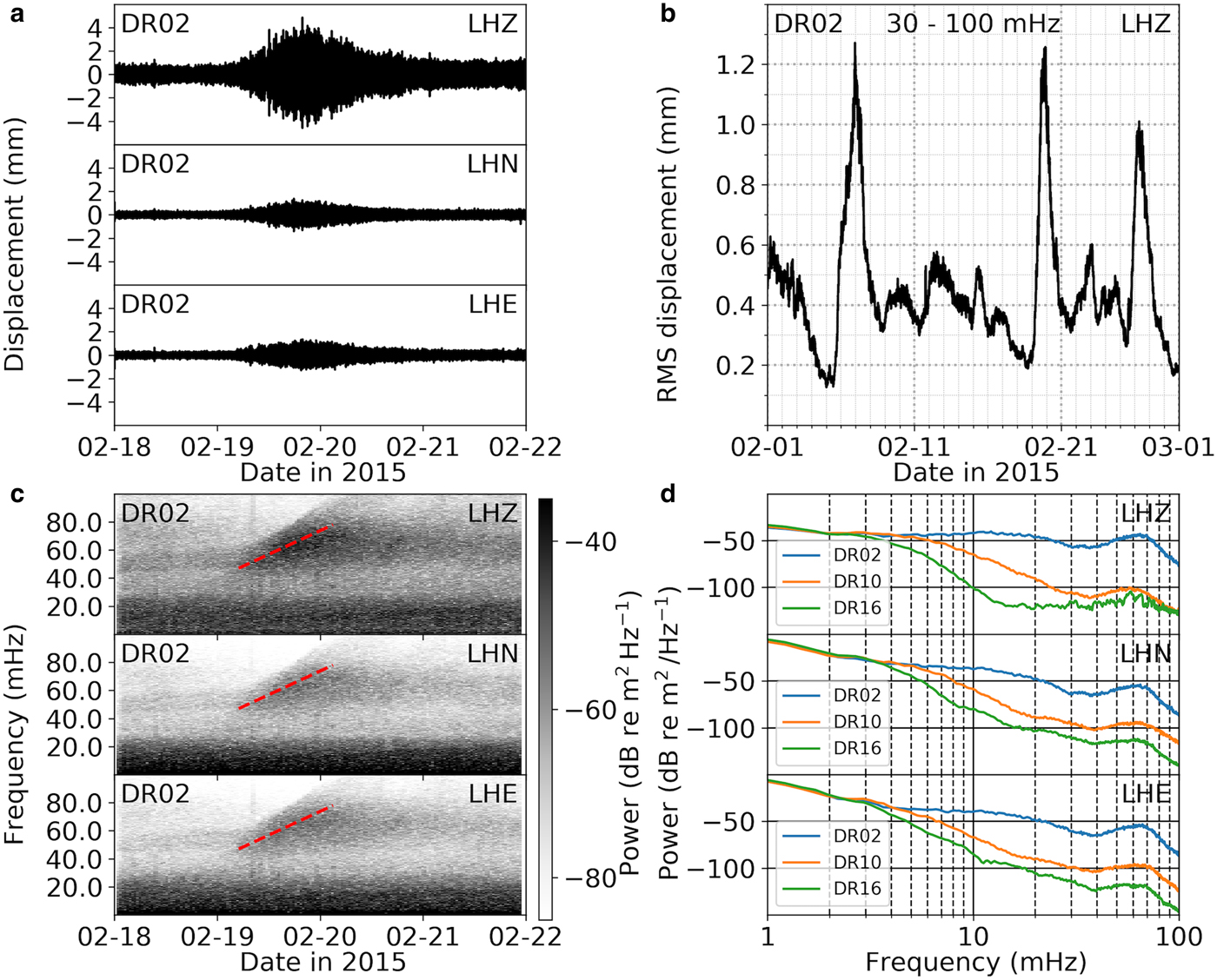
Fig. 6. RIS response to a swell event from 02:00 on 19 February to 10:00 on 21 February, 2015: (a) 4-day seismograms at DR02 (bandpassed 30–100 mHz). (b) RMS of the vertical displacements at DR02 (bandpassed 30–100 mHz) in February 2015. RMS window length is 4096 s. (c) Displacement spectrogram at DR02. The dispersion trend slope (red dashed) indicates a source distance of ~2000 km. (d) Displacement spectrum at DR02 (blue), DR10 (orange) and DR16 (green) from 19 February 02:00 to 21 February 10:00. The vertical LHZ and horizontal LHN and LHE components are indicated in each subplot.
Ice shelf vibrations excited by swell impacts show significant attenuation away from the ice front (Figure 6, Bromirski and others, Reference Bromirski2017). Swell-band amplitudes were much higher at the ice-front station (DR02) than at non-ice-front stations (DR10, DR16) (Fig. 6d). The rapid power decrease away from the ice front was in part due to the decay of evanescent modes and/or damped traveling flexural-gravity wave modes. Vertical displacements (LHZ) decayed faster than horizontal components (LHN for north-south, LHE for east-west), revealed by the greater attenuation from DR02 to DR10 on the LHZ channel than on the LHN channel. There are two possible reasons: (1) ice-shelf vertical vibration energy can leak into the water layer, or (2) the vertical component may contain more evanescent and/or damped traveling energy. The spectrum of the vertical component at DR16 was augmented by the local transient events that masked the attenuation from DR10.
5.1.2. Source direction and dispersion
Beamforming shows that the dominant source directions were between NNE and NNW, pointing to the shelf front (Fig. 7a,b). Although swell energy is predominantly in the 30–100 mHz band, coherent plate waves were also observed below this band. In particular, flexural-gravity waves were observed well below 20 mHz. This is confirmed by the close agreement between the beamformed dispersion curve and the theoretical flexural-gravity wave dispersion relation (Fig. 8). Both the radial and vertical components show coherent energy. Below 20 mHz, the frequency of the peak power in Fig. 8b was 2.9 mHz at the slowness of 15 s km−1, giving a phase speed of 66.7 m s−1. The flexural-gravity wave horizontal motions were much larger than the vertical motions, resulting in part from the horizontal motions of the forcing gravity waves being much larger than the vertical motions at low frequencies (Fig. S3). The rough base of the ice shelf facilitates coupling of gravity-wave horizontal forcing into flexural-gravity waves, resulting in relatively large horizontal motions.
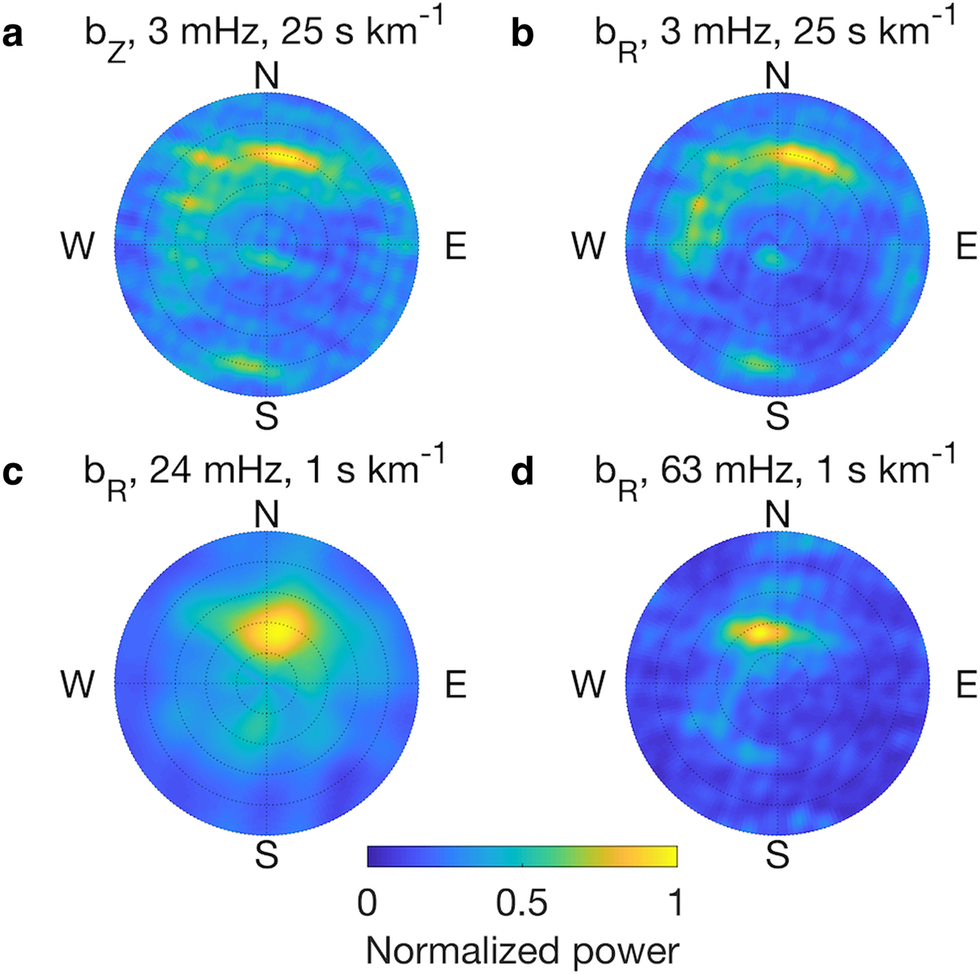
Fig. 7. RIS response to a swell event from 02:00 on 19 February to 10:00 on 21 February, 2015: Phase-only beamforming of (a) the vertical component at 3 mHz and the radial component at (b) 3, (c) 24 and (d) 63 mHz. For each subplot, the azimuth corresponds to the signal incoming direction, while the radial axis represents slownesses that vary from 0 at the center to the maximum slowness given in each subplot title. The peak-power regions give dominant signal incoming directions and slownesses. The signal incoming directions are clear and characteristic at these selected frequencies. Processing FFT window length is 4096 s, with step size of 2048 s. Beamforming power levels are normalized to the maximum value at each frequency in each subplot.
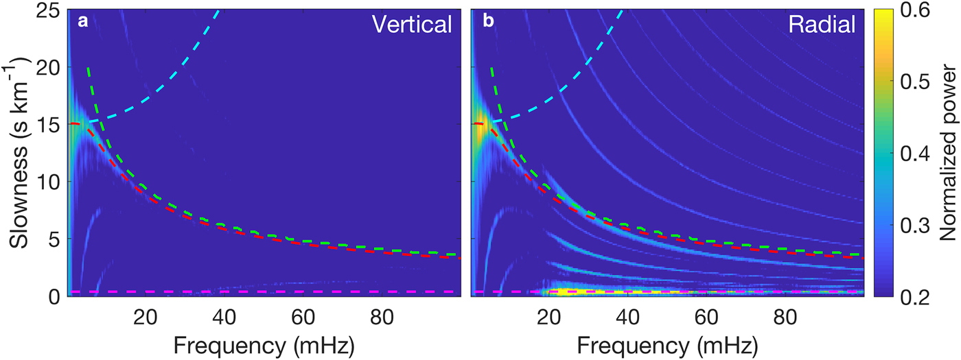
Fig. 8. RIS response to a swell event from 02:00 on 19 February to 10:00 on 21 February, 2015: Dispersion curves of (a) vertical and (b) radial components, obtained by averaging the beamforming output over 0° to 20° azimuth (the north-south line subarray is roughly along 10°). Phase speed dispersion curves of ocean surface gravity waves (cyan), flexural waves (green), flexural-gravity waves (red) and  $S_0^\ast $ (magenta) in the AIWB model (see Fig. 3) are overlaid for comparison. The subplots are normalized to the maximum value over the two subplots.
In the 20–100 mHz band, the dominant slowness was between 0.3 and 0.4 s km;−1 without observable dispersion, consistent with  $S_0^\ast $ propagation (Fig. 8). The dominant source direction was from the NNE at lower frequencies and NNW at higher frequencies (same for the 28 strongest swell events from January to October 2015), possibly due to the variability of the dominant swell impact region along the ice front (Fig. 7c, d). The frequency of the peak power was 53 mHz, and the corresponding slowness was 0.34 s km;−1, giving a phase speed of 2.94 km s−1 (Fig. 8). The radial component was more coherent than the vertical component, consistent with the theoretical expectation that $S_0^\ast $ has horizontal motions much larger than vertical motions.
A spectral peak in the swell band was observed between 60 and 70 mHz on both vertical and horizontal components (Fig. 6d). Although extensional Lamb waves were observed on the radial component in the beamforming analysis, coherent flexural waves were not observed on any component in this band, suggesting that the spectral peak of the vertical component was due to loss of flexural wave coherence. Based on the dispersion curves in Fig. 5a, the wavelengths of the flexural waves (purple) in the 20–100 mHz band are 2.8–5.3 km (280 m s−1/100 mHz = 2.8 km, 106 m s−1/20 mHz = 5.3 km), while the wavelengths of the flexural-gravity waves (green) at 3 mHz (not shown) are ~22.2 km (66.6 m s−1/3 mHz = 22.2 km). The shorter wavelengths in the 20–100 mHz band resulted in the flexural waves being less coherent in that frequency band, likely in part a consequence of the larger station spacing (5–20 km) compared with the signal wavelengths.
Beamforming analysis for the 28 strongest swell events from January to October 2015 indicates that flexural-gravity waves were always observed below 20 mHz, with extensional Lamb waves occurring above 20 mHz. OASES modeling (Fig. S4) shows that both flexural waves above 20 mHz and extensional Lamb waves below 20 mHz can propagate in a 300 m ice layer coupled with a 400 m water layer above the seafloor, the AIWB model (Fig. 3). Therefore, the dominance of a particular wave type was likely due to the ice-water coupling described in the plate wave generation mechanism rather than due to the model structure constraints on wave propagation.
As an additional verification, north-south (NS) and west-east (WE) subarrays are chosen to study the wave propagation direction and group speed with cross-correlation. Below 5 mHz, the dominant coherent signal, flexural-gravity waves, were non-dispersive. In other words, group speed was equal to phase speed and was constant in this band. A coherent signal propagating southward at ~66 m s−1 group speed was indicated by the 2–4 mHz filtered CCFs of the LHZ and LHN components (Fig. 9a,b), consistent with the beamforming analysis. In the 20–100 mHz band, the dominant coherent signal, extensional Lamb waves, were non-dispersive. A coherent signal propagating southward at ~3.2 km s−1 was indicated by the 20–100 mHz filtered CCFs of the LHN component (Fig. 9c), consistent with the beamforming analysis. No coherent signal was observed in the west-east direction (Fig. 9d). The high peaks of CCFs with small station separations are due to waveform similarity at nearby stations.
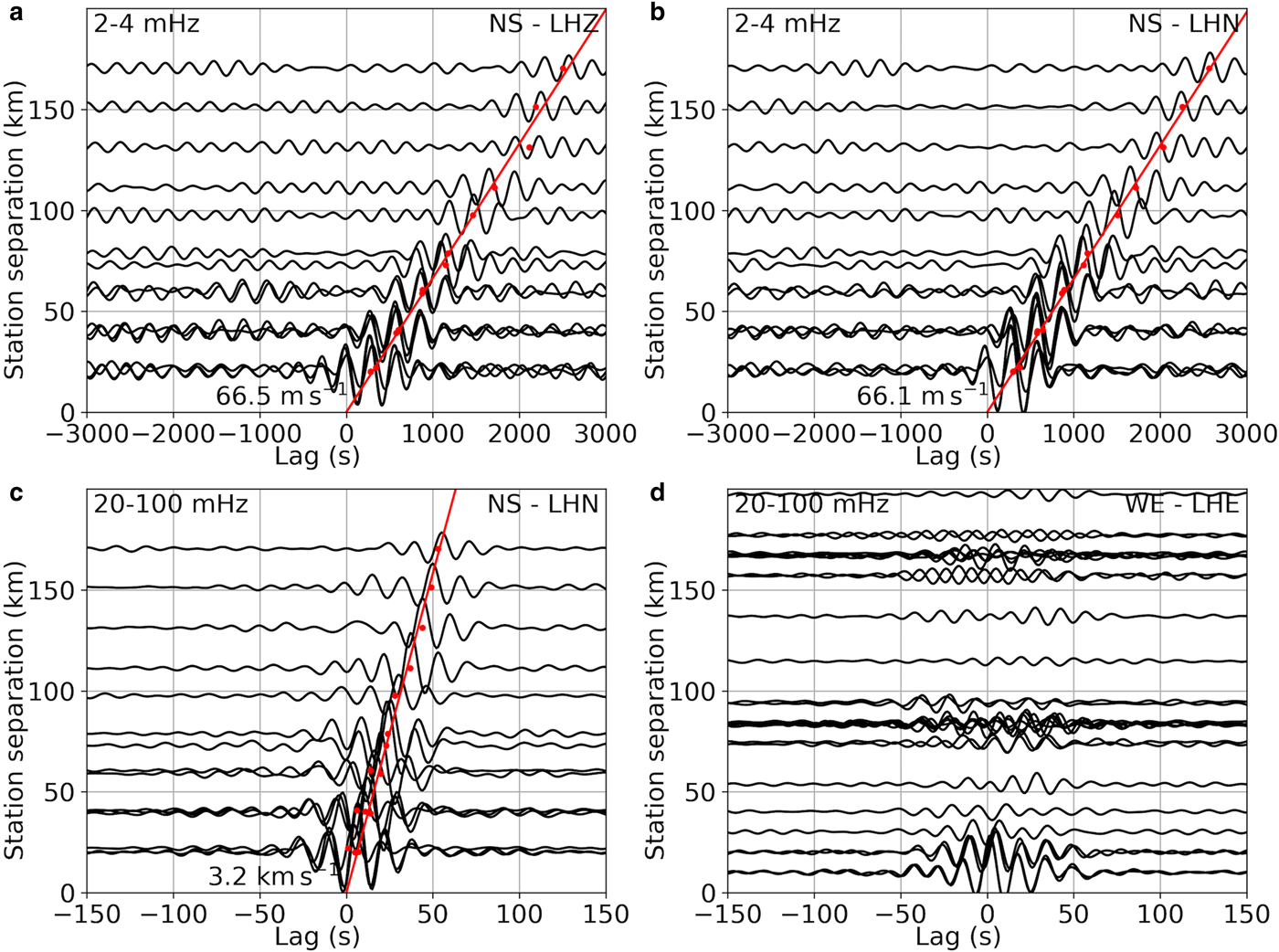
Fig. 9. RIS response to a swell event from 02:00 on 19 February to 10:00 on 21 February, 2015: (a) Cross-correlation functions of the LHZ channel between north-south (NS) subarray stations (DR05, DR06, DR10, DR14, DR15, RS16) (bandpassed 2–4 mHz). (b) Cross-correlation functions of the LHN channel within NS subarray (bandpass filtered, 2–4 mHz). (c) Cross-correlation functions of the LHN channel within NS subarray (bandpassed 20–100 mHz). (d) Cross-correlation functions of the LHE channel between the west-east (WE) subarray stations (RS01, RS02, RS03, DR07, DR10, RS04, DR11, RS05, RS06, RS07) (bandpass filtered, 20–100 mHz). The raw data were demeaned, filtered and cross-correlated between each station pair in time domain. The peak positions of the cross-correlation function envelopes are indicated by red dots, which are fitted by the red line constrained to go through (0, 0).
5.1.3. Particle motion
The azimuth, incident angle and ellipticity of the maximum particle motion polarization during the swell event was obtained for DR02, DR10 and DR16 (Fig. 10), which were ~2 km, ~100 km, ~300 km south of the ice front, respectively. Particle motions at non-ice-front stations (e.g. DR10, DR16) had the following patterns: (1) The source azimuth was northerly, changing from NNE to NNW with increasing frequency in the 20–100 mHz band, consistent with the beamforming analysis and with the expectation that swell impacting the shelf front excites these signals. (2) Below 10 mHz, incident angle variability indicates that the maximum polarization was horizontal, due to coupling with the shallow-water gravity waves that have mostly horizontal particle motions. In the 20–100 mHz band, the maximum polarization was horizontal, characteristic of extensional Lamb waves. Estimates of the incident angle (Fig. 10b) in the 10–20 mHz band at DR10 have a wide range, possibly indicating a transition band between flexural-gravity wave domination and extensional Lamb wave domination. (3) Ellipticity analysis (Fig. 10c) indicates that the maximum polarization was an oblate ellipse both below 10 mHz and in the 20–100 mHz band. Combining the ellipticity and incident angle distributions, the major axis of the oblate ellipse was horizontal in both frequency bands. In the 10–20 mHz band, the polarization was close to circular as a result of low signal-to-noise-ratio that affects horizontal/vertical ratios in the transition band.
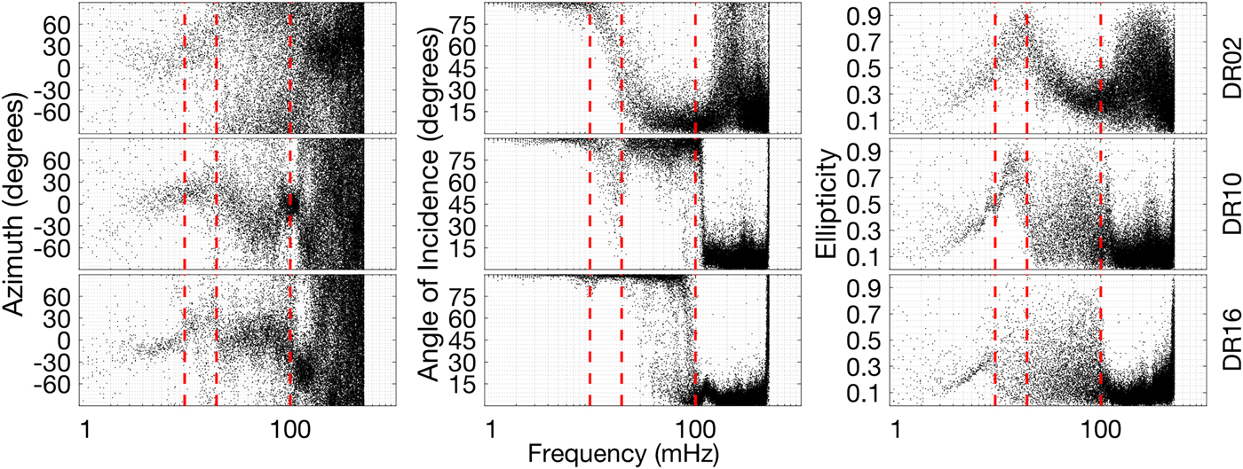
Fig. 10. RIS response to a swell event from 02:00 on 19 February to 10:00 on 21 February, 2015: Frequency-dependent azimuth (left column), angle of incidence (middle column) and ellipticity (right column) at DR02 (top row), DR10 (middle row) and DR16 (bottom row). The time series were partitioned into 16384 s (4 h 33 min 4 s) windows overlapped by half window length, resulting in a frequency-bin width of 60 μHz. Each dot represents the estimated parameter in that time window at the corresponding frequency bin. The three vertical red dashed lines indicate 10, 20 and 100 mHz, respectively.
Particle motions at ice-front stations (e.g. DR02) differed from those at non-ice-front locations in the following respects: (1) The source azimuth cannot be constrained well at the ice front and (2) the maximum polarization was vertical in the 20–100 mHz band at the ice front. Both observations could be the effect of the evanescent modes and/or the damped traveling modes of flexural-gravity waves that were not observed at non-front stations.
These observations indicate that the dominant signal propagated roughly north to south, away from the shelf front. Therefore, linear, prograde and retrograde particle motions correspond to 0, negative and positive phase difference between the vertical component and the north component, respectively. This vertical-north phase difference was frequency dependent, shown in Fig. 11. The positive phase difference in the 1–10 mHz band indicates retrograde particle motion, consistent with flexural-gravity-wave propagation (Robinson, Reference Robinson1983). The phase lag changed significantly in the transition band, i.e. 10–20 mHz and dropped to near 0 above 20 mHz at stations south of DR06, probably due to the vertical component decaying below the detection level. The phase lag at stations north of DR06 was positive and > 40° above 20 mHz, indicating retrograde particle motion, which is consistent with extensional Lamb wave propagation.
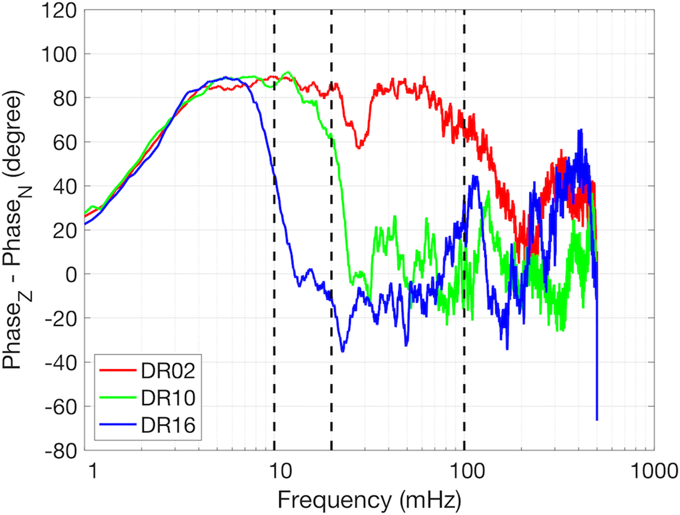
Fig. 11. RIS response to a swell event from 02:00 on 19 February to 10:00 on 21 February, 2015: Frequency-dependent phase lag between vertical component and north component at selected stations. Positive lags indicate retrograde motions. Negative lags indicate prograde motions. Zero lag indicates linear polarization or a noisy time period. The time series were partitioned into 2.28 h windows, with a half window-length overlap. The phase lag is calculated by averaging the phase difference between FFTs between the vertical and north components over all windows. To identify dominant features, the phase lag curve was then smoothed by 20-point moving average. The three vertical black dashed lines indicate 10, 20 and 100 mHz, respectively.
5.2. Plate waves excited by tsunami and IG waves
Plate waves were also observed during tsunami impacts between 17 and 19 September 2015 and during a strong IG arrival between 5 and 8 May 2015 (Bromirski and others, Reference Bromirski2017). Coherent extensional Lamb waves were not observed during tsunami excitation, but were observed in the 20–30 mHz band during the IG event. Low energy levels above 20 mHz during the tsunami explain this difference. However, flexural-gravity waves were observed below 20 mHz, similar to that observed during the swell event. Importantly, flexural-gravity waves were observable even during most ‘quiet’ days both in spectra and in beamforming analysis, indicating that flexural-gravity waves were generated continuously by the persistent IG waves throughout the year. These year-round vibrations can potentially weaken the ice by expanding existing fractures (Holdsworth and Glynn, Reference Holdsworth and Glynn1978; Bromirski and others, Reference Bromirski2017).
6. DISCUSSION
Gravity-wave amplitudes are expected to vary considerably along the Antarctic coast, with associated forcing on ice shelves dependent on the source amplitude, location, spectral content and continental shelf bathymetry. Continuous gravity-wave impacts promote crack expansion and iceberg calving, facilitating the progressive reduction of ice shelf buttressing over time. VLP, IG and swell synoptic variability associated with individual storms will differentially impact different regions along the Antarctic coast at different times. Year-round ice shelf seismic records at the RIS and PIG ice shelves allow inferences about the general characteristics of gravity-wave spatial variability and their impact (Fig. 12).
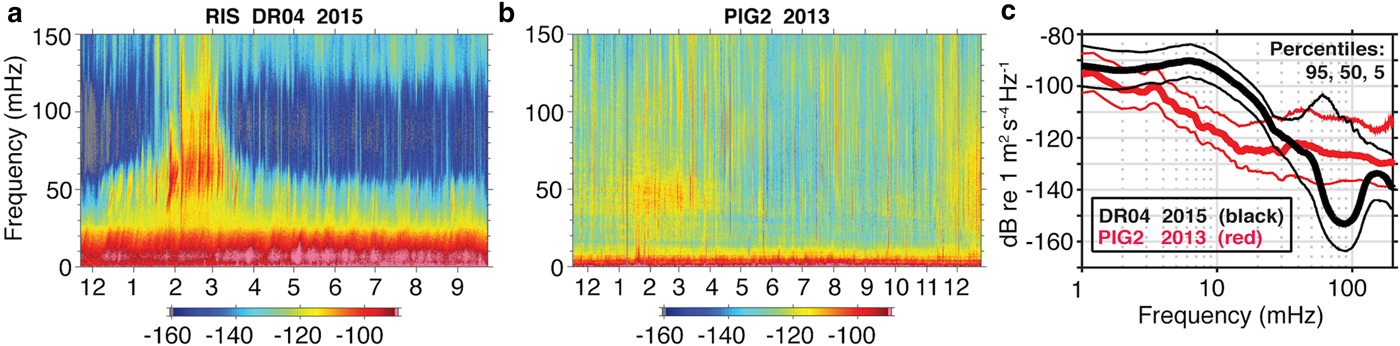
Fig. 12. Acceleration response power spectral density spectrograms (in dB re 1 m2 s−4 Hz−1) at (a) RIS seismic station DR04, located ~50 km south of the RIS ice front and at (b) the PIG2 seismic station ~24 km east of the PIG ice shelf front, collected as part of the Observing Pine Island Glacier project (Holland and Bindschadler, Reference Holland and Bindschadler2012). Months are indicated by the x-axis tick labels. (c) Spectra with percentile spectral levels obtained at DR04 and PIG2 for the time periods of the spectrograms shown.
Noticeably lower spectral amplitudes were observed at PIG during January to March 2013 in the swell band (30–100 mHz) (Fig. 12), which we hypothesize is due to PIG being partly shielded from Amundsen Sea wave activity mainly by the Thurston Island, the King Peninsula and the Canisteo Peninsula. Also, the PIG ice shelf front is oriented roughly north-south (orthogonal to the West Antarctica coast). Typical eastward storm tracks would tend to result in oblique gravity-wave approach angles to PIG shelf front, which could reduce the response. The higher spectral levels at PIG compared with RIS in the austral winter at frequencies >60 mHz can be explained in part by PIG being farther north where sea-ice cover is typically less and not as persistent, so the overall winter damping of swell is less. These location-related differences result in the comparatively high amplitude spectral levels at RIS during February, represented by the 95th percentile peak at DR04 near 60 mHz (Fig. 12c). These factors combine to produce more low-level background energy at PIG, while sea-ice north of the RIS front damps the shorter period gravity-wave energy at DR04 at frequencies >60 mHz during the austral winter. Importantly, Thwaites, Dotson, Getz and other West Antarctic ice shelves are more exposed than PIG to gravity waves coming from the open waters of the Amundsen Sea, which should result in higher-amplitude gravity waves at certain coastal locations compared with PIG.
The apparent year-round persistence of VLP band energy at both RIS and PIG suggests that this forcing is common at all ice shelves. Spectral levels are higher at the RIS at <20 mHz, but VLP band energy is also present at PIG. Presumably, flexural-gravity waves are the source of the energy at PIG in this band, although the PIG array aperture precludes identification of VLP signals with beamforming. Note the much higher IG band peak levels at RIS (about 20 dB higher) compared with PIG near 6 mHz, likely resulting from less flexural-gravity wave energy at PIG.
As the PIG ice shelf is shielded by the northern promontories and the PIG front is oriented roughly north-to-south, swell events likely rarely excite strong vibrations of the PIG ice shelf. Only one clear swell event was recorded during the 2013 austral summer from 12 March 12:00 to 14 March 00:00. The same analysis methods used for the RIS observations were applied to the PIG seismic data. Coherent signals from the west were identified above 20 mHz on the vertical component (Fig. 13), consistent with generation at the PIG shelf front. The slowness resolution is low due to the small array aperture. Thus, it cannot be determined whether coherent signals exist below 10 mHz. However, in contrast to the RIS, dispersion curve analysis of the vertical component at the PIG ice shelf shows that flexural waves exist above 20 mHz (Fig. 14a) in addition to flexural-gravity waves below 20 mHz (Fig. 14a) and extensional Lamb waves (Fig. 14b). Flexural waves are detected at the PIG ice shelf in part because the PIG seismic array is close to the ice front (~25 km) so that the flexural waves are less attenuated, and also because the relatively small station separation of the PIG array (~1–2 km, less than the flexural wave wavelengths) allows identification of coherent signals from the shorter-wavelength higher-frequency swell-induced flexural waves.

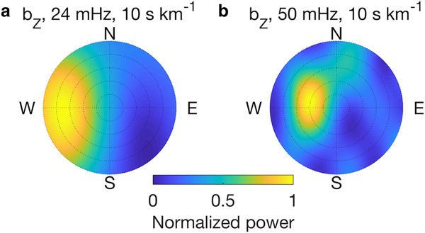
Fig. 13. PIG ice shelf response to a swell event from 12:00 on 12 March to 00:00 on 14 March, 2013: Phase-only beamforming of the vertical component at (a) 24 mHz and (b) 50 mHz. For each subplot, the azimuth corresponds to the signal incoming direction, while the radial axis represents slownesses that vary from 0 at the center to the maximum slowness given in each subplot title. The peak-power regions give dominant signal incoming directions and slownesses. The signal incoming directions are clear and characteristic at these selected frequencies. Processing FFT window length is 4096 s, with step size 2048 s. Windows with missing data are discarded. Beamforming power levels are normalized to the maximum value at each frequency in each subplot.
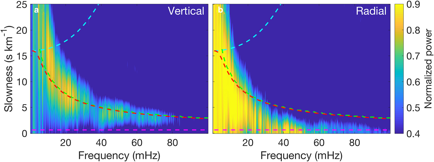
Fig. 14. PIG ice shelf response to a swell event from 12:00 on 12 March to 00:00 on 14 March, 2013: Dispersion curves of (a) vertical and (b) radial components, obtained by averaging the beamforming output over 260° to 280° azimuth (20° azimuth range centered due west). Phase speed dispersion curves of ocean surface gravity waves (cyan), flexural waves (green), flexural-gravity waves (red) and  $S_0^\ast $ (magenta) in the AIWB model (see Fig. 3) are overlaid for comparison. An ice thickness of 460 m and a water depth of 400 m were used to compute the dispersion curves, representing the PIG ice shelf geometry at the array area (Fretwell and others, Reference Fretwell2013). The subplots are normalized to the maximum value over the two subplots.
Flexural-gravity wave energy attenuates with distance from an ice shelf front, but observations indicate that there is still substantial wave-induced energy 100 km from the RIS front (Bromirski and others, Reference Bromirski2017). Significantly less flexural-gravity wave energy is observed at larger ranges from the front such that much of the RIS is little affected by this forcing. In contrast, smaller ice shelves, such as the PIG ice shelf, Thwaites ice tongue and Dotson and Getz ice shelves, have grounding zones that are on the order of 100 km or less from their fronts. Thus, for smaller shelves, the entire shelf is subjected to flexural-gravity wave forcing and associated fracture expansion, as well as potentially affecting grounding zone stability.
7. CONCLUSIONS
We deployed a 34-station seismic array on the RIS from November 2014 to November 2016 to study its response to long-period gravity-wave impacts. Between January and October 2015, we observed 28 non-overlapping strong swell events. For one of the strongest events (February 2015), we observed two types of plate waves: dispersive flexural-gravity waves below 20 mHz and non-dispersive extensional Lamb waves in the 20–100 mHz band, both propagating landward from the RIS front. Seismic array beamforming revealed that flexural-gravity waves, propagating at close to shallow-water gravity-wave speeds, dominated the coherent signal below 20 mHz. However, coherent flexural waves were not observed at RIS in the 20–100 mHz band even though vertical motions were strong, probably because the station spacing of the RIS beamformed subarray (5–20 km) is significantly longer than the wavelengths of flexural waves (2.8–5.3 km) in the 20–100 mHz band, resulting in lower coherence between stations.
We compared the response of the large stable RIS with the PIG ice shelf using seismic data collected by a 5-station array deployed on the PIG ice shelf from January 2012 to December 2013, with the PIG array located closer to the ice front than the RIS beamforming array and with smaller station spacing. In contrast to RIS, beamforming of the PIG seismic data showed evidence of flexural waves above 20 mHz, likely detectable because of the smaller station spacing. Lower flexural-gravity wave spectral levels in the IG band at the PIG ice shelf compared with the RIS indicates that less gravity wave energy impacts PIG, partly due to the orientation of the PIG ice front relative to IG wave propagation direction and shielding by northern promontories.
Our results improve the understanding of the response of Antarctic ice shelves to long-period gravity wave forcing. We conclude that because of the ubiquitous storm activity in the Southern Ocean, most, if not all, West Antarctic ice shelves are likely subjected to gravity-wave impacts that excite plate waves. However, significant differences in gravity wave forcing are expected as a result of storm track and storm intensity, as well as the orientation of the ice front relative to gravity wave arrivals and the shielding of ice shelves by promontories. In this respect, it seems likely that the Thwaites Glacier tongue, Dotson, Getz and other Amundsen coast ice shelves are more exposed than PIG to gravity waves arriving from the north. Persistent excitation of relatively high-amplitude flexural-gravity waves induce dynamic strains that can expand existing fractures and thus affect ice shelf integrity and their evolution.
SUPPLEMENTARY MATERIAL
The supplementary material for this article can be found at https://doi.org/10.1017/jog.2018.66
ACKNOWLEDGMENTS
Bromirski, Gerstoft, Chen and Diez were supported by NSF grant PLR 1246151. Stephen was supported by NSF grant PLR-1246416. Wiens, Aster and Nyblade were supported under NSF grants PLR-1142518, 1141916 and 1142126, respectively. Seismic instruments and on-ice installation support were provided by the Incorporated Research Institutions for Seismology (IRIS) through the PASSCAL Instrument Center at New Mexico Tech. The RIS and PIG ice shelf seismic data are archived at the IRIS Data Management Center, http://ds.iris.edu/ds/nodes/dmc/, with network code XH and XC, respectively. The facilities of the IRIS Consortium are supported by the National Science Foundation under Cooperative Agreement EAR-1261681 and the DOE National Nuclear Security Administration. We thank Helen Fricker and two reviewers for helpful comments. We thank Patrick Shore, Michael Baker, Cai Chen, Robert Anthony, Reinhard Flick, Jerry Wanetick, Weisen Shen and Tsitsi Madziwa Nussinov for their help with field operations. Logistical support from the US Antarctica Program in McMurdo was critical and is much appreciated.


 Open access