


Introduction
Since the beginning of the century glaciologists have spent considerable effort to measure emergence of ablation stakes, yet, nevertheless, no good statistical treatment seems to have been published hitherto. This ought to be done in order to complete incomplete sets of data, to give adequate rules for their implantation, and to know the accuracy of the total mass balances calculated for the whole glacier. If some theory of glacier fluctuations such as Nye’s is applied to field data, it is desirable to know the “noise” which enters in the input (the yearly balances).
As we shall see a comprehensive statistical treatment needs first a better definition oi the balance, and a close examination of the sources of error in the measurement. It will appear that these random terms in the balances are not independent. For this reason the classical computation of marginal variances would be incorrect here. More advanced statistics and matrix calculus are needed.
We have now at our disposal annual balances for 16 consecutive years (1956–72) on the ablation area of Glacier de Saint-Sorlin (French Alps). The Glacier de Saint-Sorlin, at the northern end of Grandes Rousses (lat. 45° 11’N., long. 6° 10’ E.) flows from the Pic de l’Étendard (3 463 m) towards the north-east. Its ablation area, approximately 900 m wide and 1 400 m long today (it has receded of 700 m since the first survey by G. Flusin, in 1905). is smooth and almost without crevasses. It can be reached with caterpillar vehicles, and a small but has been erected close to it by the Laboratoire de Glaciologie in 1969.
Glaciological work began in 1957, under the impulse of C.-P. Péguy. In June of that year four ablation stakes of Kasser’s model were driven with a hot-water drill lent by P. Kasser. In 1959, with a copy of Kasser’s hot point, the present author could increase the number to 10. Only 3 or 4 holes could be drilled at that time between sunrise and sunset!
With poor means and unpaid collaborators, the survey of stakes went on each year. Among them, let us call to mind the memories of the late J. Corbel, killed in a road accident during a speleological field trip in Spain, and of the late R. Vivet, who fell to his death when climbing the Aiguille Verte with 14 other aspirants to the title of guide οf the French mountaineering school in July 1964.
That year the C.N.R.S. founded its Laboratoire de Glaciologie and the glaciological work could proceed with a permanent staff. In 1966, with a steam drill devised by F. Gillet, which can drill a hole 10 m deep in 20 min, the number of ablation stakes was raised from 11 to 22. Since 1968 an engineer in topography and geodesy, C. Carle, has joined the staff. In the years 1967–70 four big missions were carried out (42 1 man-days and 10 tons of material for the summer of 1969). In recent years the use of light aircraft and a snow scooter has considerably reduced the logistic burden. This paper is the first analysing the many data which have been collected.
This historical record explains why, in spite of considerable effort, the table of balance values (32 different sites and 16 calendar years) is far from being complete. Moreover in some years of unusual ablation, stakes were lost. In other years some stakes remained hidden under fresh snow at the time of the survey; then only a balance for two or more years is known. We have at our disposal only 194 field data to fill the 512 compartments of the table (38%).
Field Procedure
The ablation stakes used by the Laboratoire de Glaciologie are made from young stems of chestnut, sold already painted as slalom stakes. They are cut in lengths of exactly 2 m, and joined together by small strings nailed on the side. When driven into a bore hole, these sticks can neither overlap nor remain slightly apart. One stake is formed by five 2 m sticks, with the following colours, starting from the bottom: red, yellow, green, black, ringed with two colours. This procedure avoids errors when surveying the field of stakes. The emergence is measured to 1 cm, taking for the level of the glacier the mean level 0.5 m from the stake.
Only the deepest stick is anchored at its lower end into the ice by two steel strips. Then, for precise velocity measurements, the point fixed relative to the ice is well known. On the other hand, for ablation measurements, the error coming from the vertical strain of the ice Reference VallonVallon, 1968) may be important. A mean correction will be made adopting a standard value of 5 m for the driven part, and a local strain equal to the one deduced from the net of stakes. This correction is not made in the data analysed here: it will be of interest only for mass-budget studies or for correlations with meteorological variables. A random error remains, however.
When a stake is near its complete emergence, a new one may be driven very close to it. Then the correspondence between both stakes is exactly known: we shall say that they are included in the same sequence. In some cases, for instance when a supraglacial stream or a crevasse has appeared very near the old stake, the new one is driven at some distance upstream. Then we shall speak of the same site, but of a distinct sequence. In the 32 sites studied, there have been 40 sequences.
The aim is to reach the balances:
(1) in metres of ice of a standard density (0.88 Mg/m3),
(2) for a calendar year (1 October to 30 September),
(3) at points of fixed geographical coordinates,
(4) smoothed over about 1 000 m2.
This choice of the definition depends upon the problems being ultimately investigated.
(1) In order to know the changes in altitude of the glacier surface (the summit of the emerging stick having been exactly levelled), the height of melted ice is required. But since we will study the total mass balance of the ablation zone and the influence of the meteorological factors it will be necessary to have the mass balances at individual points in Mg/m3, to a constant factor.
(2) When studying correlations with meteorological variables, it is convenient to introduce monthly averages, which are already computed. Moreover, the end of the ablation season (viz. the period during which any snowfall has completely melted before the following one) changes very much in the Alps according to the year (and to the altitude in larger glaciers). Thus the only way to measure balances for a budget year in an ablation area would be to survey the stakes at the beginning of the winter, a heavy and dangerous task. Moreover, in this case many stakes would not be found.
(3) Balances in Eulerian variables are needed for calculating mass balances of the whole area, for glacier dynamics calculations and for correlations with altitude. This will not be the case for heat-balance or hydrological-balance calculations in a limited area.
(4) We are interested in the behaviour of the whole glacier, and not in very local ablation forms.
None of these requisites is fulfilled:
(1) The density of glacier ice varies by several per cent.
(2) The surveys could be done only within 10 d of the ideal date. Even in 1958 and 1959 they were done on 7 and 8 September respectively. Moreover in 1960, 1963, 1965 and 1972 newly fallen snow covered the glacier and it was not taken into account in the measurements. So the emergence data for these years refer to an anterior date, which is probably the end of the ablation season. The level of the ice at the stakes was first measured in June 1957; since the superimposed ice is negligible in June, this level refers to the end of the ablation season 1956. (These years are marked by a star in Table I.)
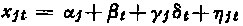
(3) The stakes move down-stream. Nevertheless, the motion is slow (Fig. 1). The horizontal movement of any stake during the period it has been surveyed is about 60 m at most, and its vertical movement about 8 m at most. In Table I, mean coordinates are given, x and y correspond to the Lambert French coordinates, after substraction of 900 000 and 320 000 respectively. The x-axis points towards the east and the y-axis towards the north, approximately.) It may be noted that, as a consequence of this motion, and of big changes of the glacier near the front, it would be in general impossible to make a good statistical analysis of very long records.

Fig. 1. The ablation zone of Glacier de Saint-Sorlin French Alps) in September 1972. Index j of the sites and movement of the stakes during the period of observation which differs according to the site). The numbers with two decimals are the estimated values of αjfor ρ = 0.
(4) The emergence relates to a glacier surface smoothed over 1 m only. Supraglacial streamlets, and changes in the dust cover and in the bubble content, cause local fluctuations in the ablation which must be smoothed out.
Some smoothing actually happens not in space but with time. The accumulation is bigger in the hollows, the ablation bigger on the hillocks. If it were not so, the smooth surface of the glacier would be unstable: ice pinnacles, pénitentes or dirt cones would appear. Thus most of the fluctuations during successive years caused by these local processes cancel each other.
It may be said that at one site fluctuations are observed in successive years with the same statistical properties as the fluctuations observed a single year over 30 or 50 m.
Symbols and Indices
In the following, italic letters denote field data such as the p-annual balance x, or integers such as p. Greek letters denote parameters included in the statistical models. A “hat” on such a Greek letter denotes an estimate of it.
Small letters denote single numbers: “real” such as x, α, β, γ, δ, ρ, σ, or integers such as m, p. the indices i, j, n, S, t, and the dummy index k.
Small capitals as N, J, T denote numbers of dimensions, of rows or columns, of degrees of freedom.
Full capitals such as A, Λ, Γ, (with the exception of W, which is a subspace, and S, Σ, which are sums) denote matrices. They may reduce to a column as X, Θ, or to a row as B, in order to represent vectors (also called X, Θ or B). M’ denotes the transpose of a square matrix M. M −1 denotes a matrix such that MM −1 = Μ −1Μ = I, I being the matrix unity. When M is non-singular, M −1 is the inverse of M. When M is singular, other conditions will be given to define M −1.
Each site has been indexed from j = 1 to j = J = 32. The order is unimportant. It has been chosen in order to have the largest possible complete block of data at the upper right corner of the table. Each successive calendar year has been indexed from t = Ι to t = Τ = 16.
The measured p-annual balances are given in Table I in metres of ice, with reversed sign (the value −0.05 corresponds to a positive balance, with superimposed ice). When p ≠ 1. because a stake has been missed some years, the p-annual balance has been inscribed in the last corresponding compartment. The 40 sequences, indexed from i = 1 to i = 1 = 40 are indicated by brackets.
Table I. Annual Balances on Glacier de Saint-Sorlin in Metres of Ice (Signs Chanced).


There are N = 194 data x n. indexed from n = 1 to n = N from left to right and top to bottom. In eight cases p = 2 and in one case p = 4. Thus j, t, i, p are known functions of n.
The Linear Model with Two Parameters
We assume a statistical linear model with two parameters. The annual balance at site j for the calendar year t is assumed to be:

where α j is a parameter peculiar to site j depending upon its altitude, aspect or other geographical factors, and β t a parameter peculiar to year t, depending upon meteorological factors, ε jt is a random variable which is assumed to be Gaussian, centred (of mathematical expectancy zero), and of standard deviation independent of j and t, Moreover we prescribe:

Thus for a p-annual balance:

where ε n is a Caussian centred random variable.
Within a sequence, the residuals ε jt of successive annual balances are not independent. They are the sum of several random errors forming stochastic series which may be classified according to their auto-correlation.
Class 1—No Auto-correlation at all
Error I: Fluctuations in the vertical strain of the glacier and in the length of the embedded part of the stake.
Error 2: Fluctuations in the density of the ice.
In these cases if the variance of an annual residual is σ 2 the variance of the sum of p consecutive annual residuals is pσ 2. The covariance of two p-annual residuals is always zero.
Class 2— Negative Auto-correlation
Error 3: Inaccuracy in the measurement of the emerged part.
Error 4: Measurement not done on 30 September.
These errors introduce opposite errors in two consecutive balances, which cancel each other when balances are added. If the variance for one emergence datum is σ′, the variance for a p-annual balance is 2σ′z, whatever p may be. The covariance of two consecutive p-annual and p-annual balances is −σ′2, whatever p and p′ may be.
Error 5: Very local fluctuations of the balance.
As explained there must be a negative feed back between two successive years, but the covariance is not so tight. We may split this error into two parts, one without any autocorrelation, and the other with the same statistical properties as errors 3 and 4.
Class 3—Positive Auto-correlation
Error 6: The stake moves with time down-stream, and then within one sequence the mean negative balance α j increases steadily with time.
Error 7: The embedded part of the stake is not vertical. The tilt increases with time, and the result is the same as for error 6.
These errors change progressively from negative to positive within one sequence, at a rate which is a random variable. Thus their covariance is strongly positive for neighbour balances at the beginning or the end of the sequence, lessens, and becomes negative for distant balances. It would be very difficult to introduce this kind of error into the model. Fortunately we may assume that it is negligible. When the displacement has become too large, the sequence has been interrupted and a new stake driven up-stream. When the tilt was important, a correction has been made. It has been checked that there was no systematic increase of the estimated residuals, as an average, within the different sequences.
Since the different errors are independent, their variances and their covariances must be added. Limiting ourselves to the errors of the first and second class, the following mathematical formulation holds. The variance covariance matrix of the ε n is σ 2Λ, the element of the (N × N) matrix in row n and column n′ being:

We have put σ′2/σ 2 = ρ. This ratio is unknown, and it is even difficult to guess some plausible value for it from what has been said.
A simpler way of defining our model would be to write it:

where this time η and η′ are Gaussian independent random variables, of respective standard deviations σ and σ′. Nevertheless in order to handle the problem it is necessary to introduce the variance covariance matrix.
A major hypothesis is that σ and σ′ (and hence ρ) are independent of n. Of course for some sites we may expect larger fluctuations than for others, but we do not know it a priori. Variances and covariances are mathematical expectancies a priori.
Best Linear Unbiased Estimate of the α j and β t
It is possible to find the best linear unbiased estimate (BLUE) of the α j and β t, denoted  and
and  , if ρ is considered as a known constant. “Best” signifies that the likelihood function is maximized; “linear” that
  and
and  are linear expressions of the x n; “unbiased” that
  = α j and
  = β t.
The data form a column vector X in the N-space and the parameters α j, β t a column vector Θ in the (J + T)-space:

Let us define a “design matrix” A of N rows and J + T columns, of element ank:

where the integers p, j, t have the values corresponding to n. Then our linear model may be written:

where Δ is a Gaussian centred random vector, the variance covariance matrix of which is σ 2Λ.
Lastly, in order to satisfy the condition given in Equation (2) we introduce the (J + T)-dimensional row vector B, of elements:

Equation (2) may be written then:

A classical theorem (Reference AndersonAnderson, 1958, theorem a.3.1) says that the likelihood function of the random vector Δ = X—A Θ is:

The BLUE  is then the vector which minimizes

and which fulfills

Taking into account that the matrices Λ and Λ−1 are symmetrical:

Putting Α′ Λ−1Α = Γ, the BLUE is given by the linear set:


The symmetrical (J+T) × (J+T) matrix Γ is singular: adding the first J rows (or columns) gives the same result as adding the last Τ rows (or columns). We shall define Γ−1 by adding the condition:

Then


As demonstrated in Appendix A, Γ−1 may in general be found by inverting a (J + T + 1) × (J + T + 1) matrix, which is not singular:

It remains to demonstrate that the best linear estimate given by Equation (18) is unbiased. We shall use the following theorem (Reference AndersonAnderson, 1958, theorem 2.4.4):
“If X is a Gaussian random vector in the N-space with mathematical expectancy and variance covariance matrix M, and D is a (Ν × N) matrix of rank N′ ≤ N, then DX is a Gaussian random vector with mathematical expectancy D and variance covariance matrix DMD′.”
Here D is the (J + T) × N matrix Γ−1A′Λ−1. The mathematical expectancy of X is X = A Θ. Then the mathematical expectancy of DX is:

Moreover the variance covariance matrix of  is:
is:

Confidence Ellipsoid of  , Supposing ρ Perfectly Known
 , Supposing ρ Perfectly Known
From Equation (15), where Γ = A′Λ−1A it follows, by transposing both sides that

whence, by multiplying to the right by  or Θ:
or Θ:


and thus

A geometrical interpretation is easy, if we define in the N-space the scalar products of vectors U and V by:

Equations (24)–(26) mean that the vector  = X—Α
= X—Α  is orthogonal to vectors A
  and A
and A  , which are both included in the (J + T–1)-space, W corresponding to B Θ = 0 by the linear transformation A. Thus
  is included in the (N − J − T + 1)-space W ⊥ orthogonal to W. (Cf. Figure 2 where (J + T − 1) has been taken equal to 2 and N to 3.)

Fig. 2. Geometrical interpretation of the best linear unbiased estimate  . X w = A
  is the projection of vector X of the N-space on subspace W, which has J + T − 1 dimensions. Its mathematical expectancy is A
  , also included in W. In the figure N = 3 and J +T − 1 = 2.
If we give to the N-space the norm:

Pythagoras’s generalized theorem leads to:

The left-hand side may be decomposed in N independent squares; the quadratic form ϕ = ║X – A  ║2 in N − (J + T − 1) independent, squares; and the third quadratic form

in J + T − 1 independent squares. The linear terms in all these squares are distributed according to a Gaussian centred law. It follows then from classical statistics that:
(1) The estimate of σ is:

(2) ϕ/σ 2 and ψ/σ 2 are distributed according to the χ2-distribution of Pearson with (N − J − T + 1) and (J + T − 1) degrees of freedom respectively.
(3) The ratio

is distributed according to the F-distribution of Fisher–Snedecor with (J + T −1) and (N − J − T + 1) degrees of freedom.
This last result allows the determination of the confidence ellipsoid for Θ. Let c be the upper 95% confidence limit for an F-distribution:

For N = 194, J = 32, T = 16, it is found from tables that c = 1.42.
With a 95% probability (if our model is correct), Θ will be found within the ellipsoid of sub-space W:

Simplified Calculation in the Case ρ = 0
When ρ = 0 matrix Λ is the matrix unity of rank N, denoted IN. Let us consider first the case of a perfect table of data, where all the compartments are filled with an annual balance. Then N = JT. Matrix A becomes a column of J times T × (J + T)-submatrices A j where the jth column is composed of 1:

Matrix Γ is of the form:

F being a J × T matrix the elements of which are all equal to 1. It is finally found that


For an incomplete set of data, comprising some p-annual balances p ≠ 1) it is possible to calculate  by hand, using an iterative procedure. The quadratic form to minimize is:

where ∑p denotes the sum for all the p-balances inscribed in the table.
Let us share any p-annual balance into p equal parts x′ jt = x jt/p among the corresponding compartments of the table of data, (instead of inscribing the totality in the last compartment). Let h jt be then an occupancy function, equal to 1 when there is a datum in the j, t) compartment and to o when there is none. Equations  then lead to

and equations  to
to

where t 1, t 2, …, t p−1 are the years associated with year t in the same p-annual balance. The set of Equations (40)–(41) is equivalent to matrix Equation (15). Let us put:

With the modified table, Sj and St are the sums per row and per column. Σtt involves as many  as there are compartments linked by a p-annual balance with the compartments of column t. The set of Equations (41)–(42) becomes:

Starting from the initial values  for every t (and then Σj(ο) = 0), we may find a solution of this set with the following algorithm:

A few loops are sufficient to obtain limits  . Until now the condition Σ

 t(∞) and to add to every
  j(∞) the mean of the
  t(∞)
t(∞)
Computation in the General Case ρ ≠ 1
When ρ ≠ 1, none of the elements of the matrix Λ−1 is zero, and a computer is needed.
It is convenient to introduce the concept of the type of a sequence. Two sequences will be said to be of the same type if they have the same number of terms and the successive p are the same. Our 40 sequences may be classified into 15 types.
The data to introduce into the computer are:
1—The adopted value for ρ.
2—For each type of sequence (s = 1 to s = s = 15), the values of the successive p.
3—For each sequence (i = 1 to i = 1 = 40), its type s and its site j.
4—For n = 1 to n = N = 194, the corresponding values of i, t, and the rank m within the sequence. j and s can then be inferred from i, and p from m and s. The following checks are convenient:


For each type of sequence, comprising m terms, a different M × M sub-matrix may be defined according to Equation (4), say Λs. First the s = 15 sub-matrices Λ s−1 must be computed and put into a memory.
Matrix Λ is formed by a diagonal of 1 square sub-matrices equal to the corresponding Λs. Matrix Λ−1 is formed by a diagonal of the corresponding Λi−1 already computed. Matrix A is formed by a column of 1 sub-matrices of dimensions Mi × (J + T), which be denoted A i. In the same way X is formed by a column of 1 sub-vectors X t, one per sequence. Then we may compute jointly:


Next Γ−1 is computed according to Equation (20),  according to Equation (18),
  = X–A
= X–A  ,
,

and  according to Equation (31). In this way it is never necessary to handle matrices having more than (J + T) × (J + T + 1) terms.
It is convenient to check the following points as the calculation proceeds:
(d) In Γ, the sum of the j first rows (or columns) equals the sum of the last T rows (or columns).


In the particular case ρ = ∞ (σ = o), the variance covariance matrix of Δ must be written σ′ 2 Λ. The element of matrix Λ is then:

In this case Equation (31) gives  ′ instead of
  .
.
Results
The computation has been done in the Institut de Mathematique Appliquée at Grenoble with an IBM-360, for different values of ρ. The estimates  j and
j and  t are given in Table II for ρ = 0 and ρ = 1, as well as the corresponding
  (Γkk−1)½, which give an idea of the accuracy with which α j and β t are known. (Theoretically the likely error for a single parameter cannot be given, only the confidence ellipsoid for the J + T parameters has significance.) The
  j for ρ = 0 are also given in Figure 1.
Table II. Values of  j,
j,  t and the Square Root of Their Variance √Γkk−1 (The signs + before these square roots must not be taken in a strict sense. Only a likelihood ellipsoid is well defined).
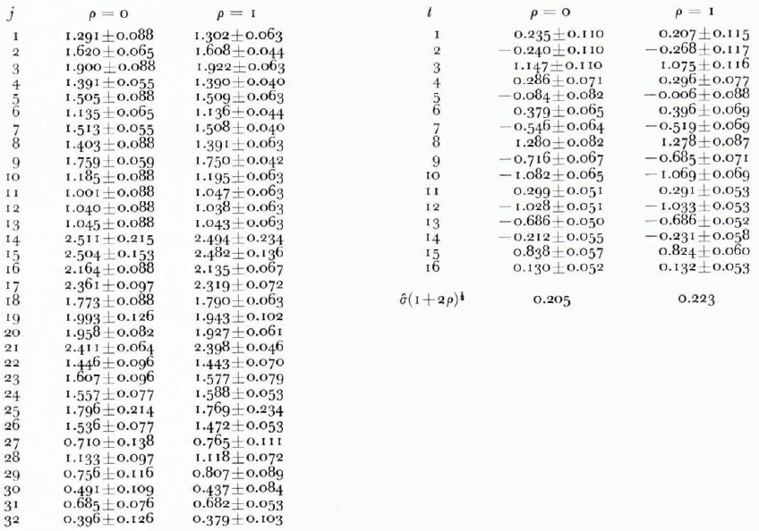
It is fortunate that the difference of the estimates for ρ = 0 and ρ = 1, is always smaller than this approximate likely error. The largest differences in the  j (for j = 19, 27, 29, 30) reach 5 cm, when the corresponding likely error is larger than 10 cm. The largest difference in the
  t (for t = 5) reaches 7.8 cm, when the corresponding likely error is larger than 8 cm. In general the
  j and
j and  t for ρ = 0 and ρ = 1 differ by about 1 cm or less. As a consequence the estimates of the residuals are very similar whichever ρ is being considered. They are given in Table III for some sequences which have particularly high residuals.
Table III. Estimateo Values of the Residuals for Those Sequences Which have the Largest Ones (First value: ρ = 0; Second value: ρ = 1).

The quantity  2 + 2
2 + 2


The estimates of the residuals are never independent random variables and thus are not distributed according to a Gaussian law. Nevertheless it is interesting to examine their distribution (Fig. 3), and compare it with the Gaussian curve.

Fig. 3. Histogram of the estimates of the residuals  ]n/p for ρ = 0 and ρ = 1. They are not independent random variables and do not follow a Gaussian law, although a Gaussian curve for a standard deviation (σ 2 + 2 σ′2)½ has been drawn.
These estimates  n are in fact the N components of a Gaussian centred random vector
  , of which we have only one sample.

X has the same variance covariance matrix as ∆, that is σ 2Λ. According to the already mentioned theorem, the variance covariance matrix of the estimate  is:
is:

Choice of ρ
It is not possible to obtain an estimate of the ratio σ′2/σ 2 = ρ from our table of data based upon rigorous theory.
The BLUE  has been obtained by maximizing the likelihood function ω (Equation (11)), in which the unknown parameter σ enters. Next an estimate
  has been determined (Equation (31)). Thus we have an estimate of ω:

An incorrect procedure would be to maximize  by seeking a minimum value for ϕΝ det Λ. It is ω which must be maximized, and this condition involves ∂


We have nevertheless computed ϕ Ν det Λ for several values of ρ in the range (0, 1). As shown in Table IV, the estimate  ρ) of the likelihood function has a maximum very near zero. That we cannot have confidence in this result is proved by the fact that, starting from a subset of (12 × 6) stake values forming a complete table (j = 1 to 10, 12 and 13; t = 11 to 16),
  ρ) has this time a minimum close to zero.
Table IV. Relative Values of the Estimate of the Likelihood Function.

We may perhaps explain this discrepancy as follows. The estimates of the residuals are more strongly correlated than the true residuals. For instance if at a site j we have only a sequence of two annual balances,  j1 +
j1 +  j2 = 0. Then the covariance of these two estimates is – σ 2, while the covariance of the true residuals ε j1 and ε j2 is zero. Thus a shortening of the sequences (as made when taking a subset from the entire set) raises the apparent correlation between successive residuals, and we find a higher ρ.
We have therefore used the longest sequences formed with annual balances alone to guess a plausible value of ρ. We hope that the quantity:

will give an idea about the value of:

We have done this computation for the two sequences of 11 annual balances, the four sequences of seven annual balances and the eleven sequences of six annual balances contained in the table of data, using the estimates for ρ = 0. For ten sequences  is negative, for the seven others it is positive. For the 116 residuals, the ratio found is 0.0093, which seems not to differ significantly from zero.
A possibility would be that σ′ is important, but that the errors of class 3, giving strong positive covariances, are not negligible. Nevertheless for the three sequences giving large positive correlations the residuals do not at all increase with time.
The Variation of the Activity Index with the Value of β t is not Significant
Among the geographical factors which determine the α j, altitude is thought to be the most important. Since the altitudes z j are not random variables it would be misleading to calculate a correlation coefficient between both as erroneously done previously (Reference LliboutryLliboutry, 1968). We must speak of ∂α/∂z, where α is a function of the site, adjusted to the point values α j. The value of — ∂α/∂z near the equilibrium line is called the activity index.
It is known that the activity index is larger for maritime climates than continental ones. Thus it is plausible for it to depend upon the year. A correlation between ∂α/∂z and β t has been sought in the following way.
Let us consider the linear model:

which involves the known altitudes z j of the different sites and a new unknown parameter μ, the same for all the sites. To have a matrix formulation, let us consider the N × (J + T) matrix H, the element of which is h nk:

(j, t. and p having the values corresponding to n). The new model is:

We must find estimates of μ and Θ. If we try to minimize ║X—A Θ — μHΘ║2, the set is insoluble. The previous estimate  will then be conserved, while a reference level for the altitudes will be chosen such that the correction term μH


In particular if ρ = 0 and ρ = 1 for any n, this condition becomes:

We can now estimate μ by minimizing

whence

The problem is to know if this value  differs significantly from zero. It has been solved by Barra (Reference Barra1972). The solution is given in Appendix B in a form more accessible to non-mathematicians. Let c 1 be the upper 95% confidence limit for an.F-distribution with 1 and (N — J — T — 1) degrees of freedom:

(For N — J — T — 1 = 145, c 1 = 3.91.)
Then, considering that events with less than 5% of probability do not happen, if μ = 0 the ratio:

where

The ratio above has been found equal to only 0.456, which is well inside the confidence limits. (It will be positive even with a much narrower confidence interval.) It is said that the test μ = 0 against μ ≠ 0 is positive at the threshold of probability of 5%. Therefore model (60) with μ = 0 cannot be rejected; we cannot say that μ differs significantly from zero.
Validity of the Linear Model
In order to test the linearity of our model, it would be necessary to work out a non-linear model, to estimate its parameters, and to demonstrate that the non-linear terms introduced are not significant. This problem remains unsolved.
Let us consider the non-linear model

which allows a variation of the activity index according to the year (new parameters δ t), in a different way for each site (new parameters γ j). The ε jt′ are Gaussian centred random variables, independent from each other, with a standard deviation σ independent of j and t. In order to raise evident indeterminacies we prescribe:

The estimates of the (2J + 2T) parameters are easy to compute only in the case of a complete table of annual balances.
The upper right block of Table I j = 1 to 13, t = 11 to 16) has been used for this purpose.
Let us minimize

It is assumed that the estimates satisfy Equations (37) and (38). Then


 t have the same values as for the linear model (1) with ρ = 0. A new calculation has been done for the (13 × 6) block. The
  j,
j,  t and the residuals of the linear model ε jt = x jt —
  j;—
j;—  t are given in Table V.
Table V. Values of x jt —  j —
j —


Next Equations (72) are solved by an iterative procedure. As starting values for the  t, the values of ε jt for site j = 11 (which give the largest value of
  ) have been chosen.
Four loops were sufficient to obtain three exact figures, which are given in Table VI.
The new estimated residuals  ′ jt are definitely smaller, as well as the estimated standard deviation:

Whether this result is significant remains an open question. Even if it is significant, the gain in the representation of the balance is not sufficient to reject the much simpler linear model.
Table VI. Values Of  .
.

Conclusion
Annual balances, smoothed over a few tens of metres, may be represented by a simple linear model:

where ε jt is a Gaussian centred random variable, of standard deviation about 0.20 m of ice. Although several kinds of error contributing to ε jt are correlated, it may be assumed that the ε jt are independent from each other. Probably the negative and positive covariances more or less cancel each other.
More dubious is the assumption that ε jt is Gaussian. For instance the deposition of an avalanche or the formation of a supraglacial stream change the balance consistently by terms which are not Gaussian. Such sites must be carefully avoided when implanting stakes, yet, nevertheless, avalanches may afford an important source of nourishment to some glaciers.
The method of estimating the α j and the β t for an incomplete set of data has been given for the general case (ε jt correlated), as well as a simpler desk procedure to be used under the assumption of independent ε jt. The values of  t for successive years are simpler to obtain than the mass balance of the whole glacier and must be introduced in routine work.
We do not know if this model is also valid for the accumulation area with the same  t, but in the ablation area the
  t are independent of altitude. If it is so on the whole glacier, one of the assumptions of Nye’s theory of glacier fluctuations (Lliboutry, 1971) would be removed.
Acknowledgement
This article has benefited from long discussions with my colleague Professor Barra who induced me to make use of modern statistics and clarified several delicate points.
Appendix A Calculation of Γ−1
Equation (20) may be written:

Multiplication of matrices may be done using the submatrices as elements:


Equation (A4) is one of the equations which define Γ−1. Transposing it we obtain Γ−1Β′ = 0. Multiplying Equation (A2) to the left by Γ−1 gives:

whence

If, and only if, Г−1 is non-singular we then have

For a complex set of data this is always the case. It would not be so, for instance, if we had only two balances at the same site and ρ = 0. Then

In this case Γ−1 =  is singular and Equation (A8) is untrue;

Appendix B Generalization of Tukey’s Non-Additivity Test in order to Test μ = 0 AGAINST μ ≠ 0 in Equation (60)
We consider the estimate of X:

This model differs from the previous one because H

 . The component of H

 , if Equation (61) is not fulfilled, without introducing a new degree of freedom. Thus only the component of H
  orthogonal to W, (H
Nevertheless, the introduction of μ has raised the number of dimensions of W to J + T + 1 and then W⊥ has only N − J − T dimensions.
Barra (1972) has demonstrated that:
(1) Φ is a Gaussian centred random vector, having N − J − T independent components of the same variance.
(2) If the component of Φ in the random direction X – A  ) is denoted Ψ, since this random direction does not depend upon Φ, the ratio

follows an F-distribution with 1 and (N − J − T 1) degrees of freedom (if the direction of Ψ was fixed, it would be a classical result).
Since the projection of any vector X within W is, according to Equation (18):

the projection of vector H


and then

The component Ψ of Φ along X – A


If condition (61) is fulfilled, the second term on the right-hand side vanishes and:

and:

Even if (61) is not fulfilled,

║Φ – Ψ║2 is deduced from Pythagoras’s theorem:

whence


