Introduction

Sideways-looking airborne radar (SLAR) has been with us for some time, and its potential for ice reconnaissance has been recognized since the early 1960s. Nevertheless surprisingly little has been done to evaluate its characteristics in this respect and provide guide-lines for interpretation of the imagery. The reasons have been mainly economic and logistic, concerning the availability of the SEAR itself and the logistic problems involved in setting up an adequate ground-truth party; they do not necessarily reflect on the potential value of the technique.

There have, of course, been several studies of SLAR for ice reconnaissance, starting with excellent presentations by Reference AndersonAnderson (1966, Reference Anderson1968) which are of particular interest in the context of the present paper because the geographical area covered was very similar. Perhaps the most thorough is the work of Reference Johnson and FarmerJohnson and Farmer (1971 [b]) on data obtained during the Manhattan cruise of 1969. There is also a study of a multi-spectral SLAR experiment by Reference Ketchum and ToomaKetchum and Tooma (1973) and one in the Gulf of St. Lawrence by the Canadian Atmospheric Environment Service (Reference HengeveldHengeveld, [1972]) using the same instrument as the present study. Of these, however, only the Manhattan operation obtained any real ground truth, and this, although thorough, was taken for a different purpose and is described by the authors as “limited” in the context of the SLAR evaluation.

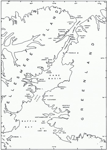
Fig. 1. Location map of Nares Strait.

SLAR has also been successfully used for tracking ice drift, both during the Manhattan cruise (Johnson and Farmer, 1971[a]) and by the Russians (Reference Loshchilov and VoyevodinLoshchilov and Voyevodin, 1972) who have developed what appears to be a rather sophisticated SLAR specifically for ice reconnaissance.

Ground truth is also conspicuously lacking in the present study, the background information being limited to tape-recorded visual observations (combined with a considerable familiarity with ice conditions in Nares Strait over four seasons), a very small amount of photography, and infrared line-scan data, some of which can be directly compared to the SLAR imagery. Owing to the poor light conditions the photographic data, though very useful in confirming interpretation, is not good enough for reproduction and none is included in this paper.

The imagery to be discussed was collected on a number of flights in a Canadian Forces Argus aircraft operated by the Maritime Proving and Evaluation Unit, Summerside, Prince Edward Island. The SLAR was a Motorola X-band AN/APS-₉₄D, and on some flights the aircraft also carried a Reconofax 13 infrared line scanner (IRLS). Some photo coverage when light conditions allowed was obtained with a Vinten 70 mm vertical camera and a hand-held 35 mm camera.

The nights covered the whole length of Nares Strait (Fig. 1) on three occasions in 1973; 13 January, 8 March, and 17 August. The March flight also covered two tracks in the Arctic Ocean, from Alert to the North Pole up the long. 62° W. meridian and thence to the ice edge down the long. 4°E. meridian. Λ further flight over Nares Strait was made on 6 April 1974, and additional material from other parts of the Canadian Arctic and the Gulf of St. Lawrence will be referred to.

Characteristics of the AN/APS-94D SLAR

The APS-₉₄D is a real-aperture SLAR which images on either or both sides of the aircraft. The blank space in the middle represents a non-imaged strip having a width of about twice the flight altitude. The ranges available are 25, 50, and 100 km a side, with corresponding scales of 1: 250 000, 1: 500 000, and 1: 1 000 000. Of these only the first two were used.

The range resolution of the SLAR is fairly constant at about 30 m, but the azimuth resolution varies with flight altitude and deteriorates across the range of the image. At 2 000 ft (610 m) flight altitude, for instance, it is 40 m at 5 km from the track and deteriorates at the rate of 8 m per kilometre. The general image quality, also, seems to deteriorate with range.

The azimuth scale depends on ground speed, which is fed into the system and the scale automatically adjusted to approximate the range scale. Another automatic correction is made for aircraft drift, but heading changes can cause serious distortions in the image geometry. A comparison of Figures 7 and 8 (p. 20a and 203) shows considerable differences in the relationship of the track to the coasts at the south end of Kennedy Channel and even in the shape of Franklin Ø0. This is because the March track was not actually straight up the channel but followed the Greenland coast, entering the picture on a heading several degrees to port of the channel axis, with a correction to starboard opposite Franklin Ø.

The horizontal distortions that occur on the imagery (e.g. at G on Fig. 3) are mostly due to heading changes, but a few are caused by altitude change or turbulence.

Optimum Range/Altitude Combination

To establish a definitive optimum range and altitude for the APS-₉₄D ice imagery it would be necessary to fly a series of combinations on the same day over the same ice. There are too many variables, both in the ice characteristics and the radar performance, for samples flown at different times and places to be conclusive. Nevertheless, in be course of a number of missions a considerable variety of combinations were tried, all of which point to the general conclusion that the lower the High t altitude the more detail of ice topography is obtained, and that the 25 km range gives more information than the 50 km. The very best detail was obtained on a brief sector of the run of 17 August 1973, with 500 ft (150 m) altitude at 25 km range. This was paid for, however, by a slightly sharper than usual falling-off of image quality down range. The usual combination used in Nares Strait was 2 000-3 000 ft (610-915 m) altitude and 25 km range; this proved satisfactory. At 4000 ft (1 220 m) and the same range the detail seemed to be less, and a very marked deterioration occurred in the imagery on 17 August 1973 when the aircraft went from 3 000 to 7 500 ft (915-2 300 in) during one run. Detail of ice topography almost completely disappeared, and total signal return from the ice decreased sharply, leaving a very dark, low-contrast image. A section flown at 5 500 ft (1 675 m) was not much better, and one at 9 000 ft (2 750 m) had parts which show practically nothing. On the other hand quite reasonable imagery was obtained from 6 000 ft (1 830 m) on 8 April 1974 (Fig. 14, p. 210).

Fig. 2. SLAR image of Hall Basin taken 13 January 1973. Range 50 km, altitude 7 000 ft (2 135 m). On this and other SLAR images the north end of the channel is at the top and the arrow shows flight direction.

From the 50 km range there are less data, as it was not used very much, but the best imagery at this range was down at 4 000 ft (1 220 m) (Fig. 9, p. 204). An attempt to use it at 1 000 ft (300 m) was a total failure; although very good discrimination was obtained in the fairly close range, more than half the range was lost altogether. At 6 000 and 7 000 ft (1 830 and 2 150m) fairly good imagery was obtained. A comparison of Figure 2 with Figure 3 shows the differences in detail between imagery at the 50 km range, flown at 7 000 ft (2 135 m) and the 25 km at 2 000 ft (610 m), both flown over the same area on the same day.

It would seem then that for maximum detail the best combination for the APS-₉₄D is the 25 km range and an altitude between 1 000 and 4 000 ft (300-1 200 m), while in cases where the extra coverage is more important than detail, the 50 km range at a rather higher altitude is preferable.

Interpretation

Most previous papers on interpretation of SLAR ice imagery have included a list of ice types with descriptions of the way they appear in SLAR imagery (Johnson and Farmer, 1971 [b]; Hengeveld, [1972]). Although these appear to be valid enough in respect to the SLAR used and the ice imaged in each case, I suggest that the practice is fraught with pitfalls for those trying to apply the criteria elsewhere. The problem is partly due to an over simplification of the characteristics of ice; all ice of a given age category does not look alike, either to the eye or to the SLAR. This is particularly true of multi-year ice, which can have very different surface characteristics according to its age and life history, but even first-year ice, although in general it is either very smooth or very rough with young ridges, can vary considerably from place to place. To radar it can also look different according to whether the ice around it is older or younger, rougher or smoother, than itself.

Even more significant is the difference between SLAR systems, particularly if they are in different frequency bands. Comparison of the imagery in the various references quoted tends to show this, quite apart from the multispectral study of Ketchum and Tooma, which deals specifically with this question. An example may be seen by comparing Figures 2-4 with Figure 6. The latter, which is copied from Anderson (1968), shows the same area at much the same time of year as Figure 4. Accompanying photographs leave little doubt that the conditions depicted are very similar, yet the SLAR used, an AN/APQ-56 operating in the K-band, shows the multi-year floes as very light, and the surrounding matrix of first-year ice, much of which is severely hummocked, hardly shows at all, giving an impression of open pack ice. In contrast the APS-₉₄D imagery shows the rough first-year ice as generally brighter than the multi-year floes.

Therefore, the statements made in this paper should be assumed to refer only to the APS-₉₄D, unless specifically otherwise stated.

Age and Thickness of Ice

Perhaps the most important feature for most ice observation purposes is the age and thickness of the ice. The Nares Strait, ice covers the whole gamut of age and thickness, from the nilas and other young stages of the North Water in Smith Sound to the heavy multi-year floes that drift down from the Arctic Ocean. There is therefore plenty of material to work on.

The ice in Nares Strait was shore-fast in both the January and March flights, and the same features can be recognized in great detail in the imagery from both. The ice falls into three basic groups: old ice floes of a great variety of sizes; very rough deformed ice which I am calling first-year, though much of it must have formed from brash ice left over from the previous summer and is therefore of composite age; and smooth ice which may be first-year or younger. There is very little coastal fast ice except in the bays, and as many of these do not break up every year, some of the ice is at least two years old. Much of it is formed from pack ice which drifts into the hays in open seasons and consolidates, and is therefore of various ages.

Fig. 3. Hall Basin, 13 January 1973. Range 25 km, altitude 2 000 ft (610 m).

Fig. 4. Hall Basin, 8 March 1973. Range 25 km, altitude 2 000 ft (610 m).

Fig. 5. Hall Basin, 17 August 1973. Range 25 km, altitude 4 000 ft (1 220 m)

Old ice

It has already been pointed out that ice of the same age does not necessarily look the same, and that this is particularly true of multi-year ice. Thus it is not surprising that the old ice does not all present the same appearance in the SLAR imagery. In this paper I propose to use the term “old ice”, which includes second-year as well as multi-year ice, as I find it impossible to distinguish between them in the SLAR imagery and to try could only be misleading.

Since X-band radar cannot penetrate the ice surface, what it records is basically the surface roughness. If an ice floe has a smooth surface it will appear dark, if it is very rough it will give a bright return. Therefore it is only in so far as age can be equated to roughness that it can be unequivocally interpreted from the SLAR image. As there is no such direct correlation, no unfailing way of determining age exists. There are, however, various characteristics which help, as will I hope be shown.

Fig. 6. Northern Hall Basin 21 April 1962, imaged by the U.S.A.F. with an AN/APQ-56 SLAR from 60 000 ft (18 300 m. (From Anderson 1963).

In actual practice it is generally not hard to separate the old ice from the first-year ice in Nares Strait in winter and spring, because it is the only ice that forms discrete floes. This, however, is due to the particular regime of the area and is not true for all Arctic channels. Old ice can be smooth or rough, gently undulating or hummocky, and therefore can vary greatly in image quality. Examples may be found in Figures 3 and 4 (floes A, B and Cc) and Figure 7 (floes A and B). Floe A m Figures 3 and 4 is a particularly interesting one. If appears to be a floe within a floe, the outer “collar” being probably younger than the inner part. This composite quality is quite common in multi-year floes. The smooth (dark) patches on the outer part of this floe are almost certainly frozen melt puddles from the previous summer. Former puddles in fact probably account for many of the dark patches on the old ice. This is certainly true of the shore-fast ice in the fiord lo the left of floes A and B. This fiord (Lady Franklin Bay) did not break up in the summer of 1972 (personal observation) but was largely covered with melt water, which was already frozen when we left the area at the end of August.

That the dark areas on these floes are in fact part of the old Hoe and not inclusions of thinner ice is shown in Figure 10 (p. 205), which includes an IRLS image of part of a multi-year floe in Kane Basin, taken on 8 March (a) and an enlargement of the SLAR image of the same floe from the 13 January flight (b). It is not usually possible to make such comparisons, as the SLAR sees only sideways and the IRLS straight down. In this case, however,as the ice had not moved in any way between the two flights and the flight tracks were not identical, it was possible to identify the IR track from the second flight on the earlier SLAR imagery. The relationship between the two pictures can be established by the two curving ridges at A. The dark patch (B) and the very bright rough patch (c) in the SLAR image both have the same cold tone in the thermal image, showing that this is not younger ice like that at point D, which has a much warmer signature and is therefore thinner (Reference PoulinPoulin, 1973).

Fig. 7. Kennedy Channel, 8 March 1973. Range 25 km, altitude 2 000 ft (610 m).

Fig. 8. Kennedy Channel, 17 August 1973. Range 25km, altitude 4 000 ft (1 220m). The differences in flight altitude between this and Figure 7 is reflected in the length of radar shadow of the islands.

The floe shown appears 10 be extremely ridgy, giving a considerably brighter SLAR signal than the surrounding deformed first-year ice. The ridges in area c are in fact detectable in the original IRLS image, though they do not appear in the reproduction. Similarly in Figure 11 (p. 206), a number of floes which appear dark on the SLAR image are light (cold) in the IRLS, indicating thick ice.

In the only sample we have of summer imagery (Figs. 5 (p. 200) and 8) most of the floes are known from visual observation to be old ice. They appear consistently darker than the surrounding brash ice, and little surface detail is visible. The large floe A in Figure 5 is described in the visual notes as a composite floe of various ages, yet it presents a rather even tone. The puddles, which were refrozen, do not show up clearly. However, all this may be due to poor radar functioning or possibly to poor choice of flight altitude (4 000 ft (1 220 m)); in the small area flown at 500 ft (150 m) (not shown) the surface detail on the floes is very much clearer, and the tonal contrast between them and the brash ice is much less.

In the Arctic Ocean imagery (Fig. 9) it is much harder to separate the old ice from the first-year, because here the pack has not been subjected to the melting and subsequent jostling of floes that has rounded and defined the edges of the old floes in Nares Strait. Nor do I have the same degree of visual back-up in this area, as the light was getting poor by the time we flew over it. However, if we accept the proposition that many of the small dark patches represent refrozen melt puddles, then most of the ice in Figure 9 should be second-year or older, and this is in fact supported by my notes, which state that at least 7/10 of the ice visible in this area was multi-year, and most of the rest very hummocky and of indeterminate age.

Fig. 9. The Artic Ocean between Alert and the North Pole, at about lat. 84º 30’ N., long. 62º 15’ W. Range 50 km, altitude 4 000 ft (1 220 m) 8 March 1973.

Old ice, then, seems to be characterized by a wide range of grey tones and may appear brighter or darker than the surrounding younger ice. It may frequently be identified by a pattern of refrozen melt puddles which appear very dark.

First-year ice

First-year ice is less varied in topography than old ice, being either undeformed and very smooth, or broken by young pressure ridges which are sharply angular and present a good targetto the radar signal. In Nares Strait this stage is usually carried to the extreme, the ice being reduced to a jumble of ridges and hummocks which appears on the SLAR image as a general bright clutter. Examples of smooth first-year ice are seen at D, E, and F on Figure 4 and at the head of the North Water (c in Figures 12 and 13). The rough first-year ice forms the “cement” that seals in the older floes over most of the channel, for example at E in Figure 10(b) and A in Figure 13. As stated above much of this kind of hummocky ice is not strictly speaking first-year, but is formed by freezing together of brash ice from the previous open season. Brash ice is represented by all the brighter areas in Figure 5. and to judge from the amount of it present at this date (17 August) it should account for a fair proportion of the hummocky ice that forms in the winter. I strongly suspect, for instance, that the ice north of Franklin ø at c in Figure 7 is of this category, with many small multi-year floes in amongst. it, such as may be seen on Figure 8 in much the same area.

Fig. 10. (a) IRLS image of ice in Kane Basin, 8 March 1973. (Dark is warm, light is cold.) Par of multi-year floe, which thinner first-year ice al D. (b) Enlarged SLAR image showing the same multi-year floe, 13 January 1973 (range 25 km, altitude 2 000 ft (610 m)).

Younger forms of ice

The main body of ice younger than first-year included in the imagery under consideration is in the North Water (Figs 12 and 13). The only other areas are the refrozen leads in the Arctic Ocean (Fig. 9) and possibly area D in Figure 3. I know from previous observations that the lead at D was not present on 15 December (Reference DunbarDunbar, 1974) so it may very well have been young ice on 13 January. Areas E and F were already there in December so must be older. Unfortunately there was a complete undercast in this area on 13 January, rendering visual observation impossible. This points up the inability of SLAR to discriminate ice thickness, as in all these areas the ice must have grown considerably thicker in the eight weeks separating Figure 3 and Figure 4, yet they look exactly the same in both. In March they had all reached the first-year stage. Similarly in the Arctic Ocean some of the leads were open, some refrozen, and some half and half, but they all look the same in the SLAR imagery.

Fig. 11. (a) IRLS image of ice in Kane Basin, 8 March 1973, showing a patch of relatively thin ice (dark) among old files. (b) Enlarged SLAR image of the same area, 13 January 1973 (range 25 km, altitude 2 000 ft (610 m)).

The North Water on 13 January was almost cloud-free, a rather rare condition, but visibility was limited by darkness. At low altitude, however, and from a first-rate look-out position, in the nose of the Argus, it is surprising how much can be seen in the dark. The visual observations, made on the southbound trip only (Fig. 12) showed an open lead about 400 m wide south of the ice edge, followed by concentrations of about 6/10 thin ice, consisting of nilas graduating southwards to grey ice. The leads and open patches tended to be oriented across the channel, and both the ice floes and leads tended to get larger as we went south.

This description is borne out by Figure 12, or at least by the parts of the imagery closest to the aircraft track; beyond about 5 km the young ice returned no signal at all in the north part of Smith Sound. On the west side of the track the edge of the fast ice shows up clearly at the extreme edge of the image, and about the latitude of Littleton Ø some returns of what look like small ridges begin to appear. On the east side there is a very interesting pattern of streaks of slush ice and small cakes. As these are wind-blown features they can only form in otherwise open water, and the grey tone, for instance between the two strings of ice at B, is a typical sea-clutter return. The cusp-like pattern of the streaks is curious and the cause of much speculation; its origin is obscure.

Figure 12 was taken on the southbound trip; on the northbound trip, exactly the same general conditions prevailed; the passage of time, however, and also the speed of drift, is illustrated by Hoe A, which appears in both images, and which moved south between the two at a speed of roughly 0.55 in s^-1. With a wind-speed of about 50 knots (25 m s^-1) recorded at our flight altitude (3 000 ft (915 m)) this works out at about the speed expected from Zubov’s rule of ice drift.

Figure 13 shows the conditions on 8 March when we had good light conditions but an almost complete cover of frost smoke, allowing only periodic vertical glimpses of the ice. From these glimpses it appeared that the ice graduated from light nilas near the head of the North Water to predominantly grey-white south of Kap Alexander. The proportion of open water decreased from north to south; near the head it was estimated through breaks in the cloud to be as high as 5/10 in places.

Figure 13 is designed to show the predominantly grey—white ice south of Kap Alexander (b) as well as the thinner ice and more open conditions to the north (a). It will be seen that the main difference between them is the heavier incidence of ridges or rafting in (b) and the presence of areas of medium grey tone in (a). The dark pieces in (a) are undoubtedly ice, and the greyer patches must presumably be the water, no doubt with new ice forming in it. Why it should appear rougher than the ice is not clear, as it would seem unlikely that the expanses of it are large enough for any appreciable sea chop to form, except in the area off the Greenland coast.

There was only a very narrow band of open water at the head of the polynya at our point of crossing. The line of the ice edge in Figure 12 is still precisely traceable in Figure 13; the expanse of light grey immediately south of this line in Figure 13 is new ice. This is confirmed by the IRLS and the vertical photography.

It will be seen that young ice forms are hard to interpret without ground truth or visual or other airborne back-up. There is very little doubt, however, that many of the questions raised could be answered by a thorough evaluation program with ground verification.

Concentration

Of the flights being considered here only the August one was concerned with concentrations less than 10/10, except for the young-ice area of the North Water. In the August imagery (Figs 5 and 8) it is not hard to measure the total concentration; the open areas appear black and all the ice various shades of grey. The situation is not quite so simple, however, in areas and times of year when young ice may be expected to be present, or when leads refreeze, as in the Arctic Ocean (Fig. 9). Here we are once again up against the problem of smooth surfaces, which can lead to real difficulty in distinguishing between ice and water, provided both are smooth.

It is often possible to discriminate between smooth ice and water by the small roughnesses that commonly appear on the ice surface and which show as faint light lines (Figs 3 and 4, areas D, E, F.). However, very similar lines occasionally appear in water openings where small amounts of brash ice are lined up by the wind. Usually, but not always, an experienced eye can tell the difference, but there remain many cases where even an experienced eye is at a loss. Many of the small black patches north of the head of the North Water, for instance (Figs 12 and 13) would be almost impossible to interpret without having seen the area. The same is true of quite a number of the smaller black areas in Figures 3 and 4, while at the scale of Figure 2 the whole smooth area might be open.

Fig. 12. Smith Sound 13 January 1973. Range 25 km, altitude 3 000 ft (915 m) showing the head of the North Water.

The best example, however, is shown in Figure 14, which consists of two samples of SLAR imagery taken on 8 April 1974. The first (a) is in Barrow Strait, where all the leads were covered with first-year ice, snow-covered and solid, whereas in the second (b), which is between Coats and Mansel Islands in Hudson Bay, the leads are all open. Without visual or other back-up information it would be virtually impossible to tell the difference.

Fig. 13. Smith Sount, 8 March 1973. Range 25 km, altitude 2 000 ft (610 m). (a) Head of North Water. (b) Area a few miles south of Kap Aleander.

Topography

Surface topography shows up on the APS-94D imagery cither as discrete bright signals or in the form of variations in grey tone. The difference in tone, for instance, between areas B and D in Figure 10(b) is probably due to minor roughnesses and undulations of the surface of B. Similarly in the same picture the overall light grey tone at E and the bright patch near C are due to the roughness of the first-year and multi-year ice respectively. In both cases the ridges and hummocks are too close together for the system to resolve. More widely spaced ridges show up as bright lines.

Fig. 14. (a) North Part of Barrow Strait, coast of Bathurst Island at top. 8 April 1974, range 25 km, altitude 6 000 ft (1 830 m) showing frozen leads. (b) Northern Hudson Bay, south-east coast, Coats Island at top. 8 April 1974, range 25 km, altitude 6 000 ft (1 830 m) showing open leads.

Without detailed ground truth it is not possible to say how reliably the ridges are picked up by the SLAR or how many are missed owing to their orientation in relation to the radar beam or other reasons. Figure 11 shows a narrow strip of relatively thin ice on the IRLS image (left of floe B) which is confirmed by photography to be smooth, but which does not appear so on the SLAR. It is oriented parallel to the radar beam about 10-15 km from the near edge of the imagery and seems to be the victim of the deteriorating azimuth resolution, which fails to distinguish it from the ridges on either side. Equally narrow strips oriented across the beam show quite clearly above floe A.

Another characteristic of this SLAR system is a variation of image quality across the range, floes tending to appear brighter close to the track. This may account for some of the tonal differences in the old floes, for example A and B in Figure 7, but most of the differences are believed to be real. Ridges and other surface features show up better in the middle and far ranges, as would be expected, the angle of incidence of the radar beam being more oblique, but there are few cases where features that show on one of the January and March pair do not appear at all on the other. (The differences between the smooth areas in Figures 3 and 4 are due to photographic factors; in the original imagery, though the quality is a little different, all the topography that appears in Figure 3 can also be seen in Figure 4). One of the very few such cases is shown al C on Figures 12 and 13, where the topographic detail in the smooth ice in Figure 13 is almost completely absent in Figure 12. As there has been no change in the shape of the feature between the two flights, there can have been no further ridge formation to account for the difference. Whether it is due to new snow cover drifting against the ridges, to relative distance from flight track, or simply to variations in functioning of the SLAR, is not clear.

Dynamic features

Because of the wide coverage obtainable with SLAR, combined with its relatively good resolution, it is unrivalled among airborne sensors for depicting dynamic features like lead orientation, shear zones and drift patterns. Lead orientation is well exemplified in the Arctic Ocean imagery and is discussed in Dunbar and Lowry (1974). Figures 2-4 show a nice example of a shear zone running from Cape Lieber to Cape Beechey between the fast ice of Lady Franklin Bay and the ice of the main channel. A similar line appears on the opposite side of Hall Basin, where fast ice has formed east of a line from Joe Ø to Kap Lupton before the main channel stopped moving. These lines are absent in Figure 5, showing that all the fast ice must have broken up in 1973.

Fig. 15. Synthetic aperture SLAR mage of the Gulf of St. Lawrence, March 1974. Altitude 37 000 ft (11 399 m) south-east Price Edward Island at left.

Drift patterns are shown in Figure 8 in the form of eddies in the lee of the islands, and in the North Water off the Greenland coast (Fig. 12).

Synthetic aperture slar

It is clear that the most serious drawback of the APS-₉₄D is its resolution, which is not adequate to resolve all necessary sea-ice features. Figure 15 is included to show that this factor is not the same with all SLARs. It shows a sample of imagery taken by a Goodyear APQ-102 synthetic aperture SLAR in March 1974 in the Gulf of St. Lawrence. The swath width is 10 miles (16 km). The resolution of this SLAR is 50 ft (15 m) and both resolution and image quality are constant across the range. The oldest ice shown is first year. Unfortunately I have no APS-₉₄D imagery of similar ice to compare it with, but its superior quality is obvious. However, the smooth-surface gremlin is still with us. The inlet at top left is undoubtedly frozen and snow-covered, yet it looks exactly the same as the open water along the coast.

Conclusions

From the evidence presented here we may conclude that SLAR has great potential as a tool for (he acquisition of sea-ice data. Although there are a number of uncertainties in interpreting the APS-₉₄D imagery, these are due mainly to problems of resolution, which, as can be seen from Figure 15, are not insoluble. Others could be solved by a thoroughly ground-truthed test programme. The only problem that may prove permanent is that of distinguishing between smooth ice and water, and even this will surely diminish with higher resolution, as with finer detail discernable the number of cases where discrimination is not possible will decrease. However, these points should be borne in mind when considering such programmes as direct provision of SLAR ice imagery to ships. In the hands of an inexperienced interpreter it could be quite misleading, as he may well tend to read it as if it were a rather fuzzy photograph, even if he is quite accustomed to interpreting the ship’s radar. Any ship receiving such imagery should have at least one trained interpreter on board.

As against these disadvantages there is the excellent coverage possible with SLAR, which provides more information with less footage of film to interpret than any other airborne sensor. This makes it a practical tool to use for repeated surveys, whether for ship operation, drift measurements, or other purpose, in contrast to photography, which is not only restricted by cloud and light conditions but requires so much flying time and produces such miles of film as to be prohibitive except in special cases. Above all there is the all-weather capability of radar, the only sensor that can penetrate both darkness and cloud.