


1. Introduction
Snow grain size is a physical property of snow that exerts controls on snow reflectance (Wiscombe and Warren, Reference Wiscombe and Warren1980), and is used to characterize mechanisms of snow metamorphism and stratigraphy (Colbeck, Reference Colbeck1991). At the surface, characterizing the snow grain size is critical for modeling snow albedo, a primary control for snow energy balance and snowmelt timing (Marks and Dozier, Reference Marks and Dozier1992). Whereas stratigraphy, or the vertical distribution of snow grain size, is critical for modeling microwave radiative transfer (Brucker and others, Reference Brucker2011) and understanding mechanical (Pielmeier and Schneebeli, Reference Pielmeier and Schneebeli2003) and thermodynamic (Hammonds and others, Reference Hammonds, Lieb-Lappen, Baker and Wang2015) properties of a snowpack.
There are multiple ways to characterize snow grain size. The classical snow grain size, defined as the largest extension (mm) of a snow grain, is most simply observed using a crystal card and hand lens (Fierz and others, Reference Fierz2009). Whereas the specific surface area (SSA) is defined as the surface area per unit volume and is measured using stereology methods. Snow grain size can also be described as an effective grain radius (r e), which is used to approximate the scattering and absorption properties of snow. Grenfell and Warren (Reference Grenfell and Warren1999) demonstrated that a collection of spherical ice particles with the same volume-to-surface area ratio as snow (i.e. characterized with stereology methods) could be used to model hemispherical reflectance. The effective grain radius is directly related to SSA by:

In the near-infrared (NIR) wavelengths (800–2500 nm), snow spectral reflectance has a characteristic decline due to the increasing absorptivity of ice at these wavelengths. Reflectance, therefore, has an inverse relationship with grain size in this wavelength range because absorption is a function of the amount of ice per unit volume. For the same snow layer, NIR reflectance typically declines over time because grain coarsening occurs due to snow metamorphism. Leveraging this relationship, methods have been developed to retrieve r e from various instruments that measure snow reflectance by relating the magnitude of NIR reflectance, or area/depth of distinct ice absorption features, to r e. Broadly, these can be classified as either discrete measurements or mapping techniques, and further characterized by the spectral range and resolution of the instrument.
At the landscape scale, remote-sensing techniques are used to map r e on a pixel-wise basis from surface reflectance. It has been shown that spaceborne multispectral sensors, like the Moderate Resolution Imaging Spectroradiometer (MODIS), can be used to map r e using band ratios or spectral unmixing (Painter and others, Reference Painter2009, Reference Painter, Bryant and Skiles2012). These satellite datasets have value due to their record length, spatial coverage and temporal resolution, but high degrees of uncertainty result from mixed pixels and low spectral resolutions. For airborne imaging spectrometers, like the Airborne Visible/Infrared Imaging Spectrometer (AVIRIS), r e is mapped at the scale of tens of meters by inverting the shape of ice absorption features resolved in spectral reflectance with radiative transfer modelling (Nolin and Dozier, Reference Nolin and Dozier2000; Seidel and others, Reference Seidel, Rittger, Skiles, Molotch and Painter2016). Spatial and spectral resolution are much higher, and uncertainty lower compared to spaceborne platforms, but due to logistics and cost, airborne datasets are very limited in spatial extent and temporal coverage.
At the local scale (i.e. laboratory, plot, snow pit) field spectrometers are used to retrieve discrete measurements of r e from surface spectral reflectance, or along the vertical snow profile (~2 cm) when coupled to a contact probe, known as contact spectroscopy (Painter and others, Reference Painter, Molotch, Cassidy, Flanner and Steffen2007). Lower spectral resolution field instruments have also been developed to measure r e from small discrete snow samples (~3 cm) using an integrating sphere and NIR light source, from which reflectance is empirically related, or calibrated, to known reflectance from a range of snow grain sizes. Examples of these instruments include DUFISSS (Gallet and others, Reference Gallet, Domine, Zender and Picard2009), IceCube (Zuanon and A2 Photonic Sensors, Reference Zuanon2013) and Infrasnow (Gergely and others, Reference Gergely, Wolfsperger and Schneebeli2014). Similarly, a vertical profiler, POSSSUM, has been developed to measure SSA profiles in one-dimension from measurements of reflectance at 1310 nm with a vertical resolution of 10 mm (Arnaud and others, Reference Arnaud2011). Discrete measurements can be time consuming to collect, are limited to instrument field of view/sample size, and cannot efficiently capture spatial variability. This can be addressed by mapping r e, which has been demonstrated using a digital NIR photographic method (Matzl and Schneebeli, Reference Matzl and Schneebeli2006). NIR photography correlates snow reflectance from 840 to 940 nm to SSA, measured using stereology methods, and is high resolution (~1 mm). However, because this method uses an empirical calibration from reflectance across a single short NIR wavelength range, it is sensitive to illumination conditions and is not easily transferable between camera sensors. Currently, there is no high spatial and high spectral resolution method for mapping r e at the local scale.
This gap is addressed here with NIR hyperspectral imaging (NIR-HSI) using a Resonon Pika NIR-320 compact hyperspectral imager and rotational stage mounted on a tripod, shown in Figure 1, to map the NIR spectral reflectance of snow. From the per pixel spectral reflectance, r e is retrieved by applying the Nolin-Dozier (N-D) scaled band area inversion technique (Nolin and Dozier, Reference Nolin and Dozier2000). To demonstrate this method, we present results from three laboratory-prepared snow samples with varying initial conditions that underwent induced melt and subsequent wet snow metamorphism. In general, when liquid water is introduced into a snowpack, snow grains begin rapid metamorphism and larger snow grains tend to grow at the expense of smaller grains (Marsh, Reference Marsh1987). By mapping r e before and after melt, we demonstrate the ability of this technique to map snow stratigraphy for a wide range of r e values. Further, it is shown that mapping r e can be used to study wet snow metamorphism processes, filling a gap in current methodologies.

Fig. 1. Laboratory setup showing a laboratory-prepared snow sample, two halogen lamps, a Resonon Pika NIR-320 hyperspectral imager and a rotational stage mounted on a tripod inside a cold room. The hyperspectral imager is located 100 cm from the exposed snow sample sidewall.
In previous laboratory experiments investigating liquid water flow through snow and wet snow metamorphism, dye tracers have been used to visualize water transport (Gerdel, Reference Gerdel1954), preferential flow channels (Schneebeli, Reference Schneebeli1995) and capillary barriers (Avanzi and others, Reference Avanzi, Hirashima, Yamaguchi, Katsushima and Michele2016). With dye tracers, the flow and pooling of water can be visualized, but quantification of grain growth with a hand lens or stereology methods is difficult and time consuming. In other laboratory work, X-ray computed microtomography (micro-CT) has been used to investigate preferential flow (Avanzi and others, Reference Avanzi, Petrucci, Matzl, Schneebeli and De Michele2017). Although snow grain size and many other snow properties can be accurately measured with micro-CT, the spatial resolution is often limited by the sample size limitations of the instrument.
In the results shown here, we demonstrate that when using the NIR-HSI method to map r e, preferential flow can be visualized, water pooling at interfaces can be identified, and grain growth at the laboratory or snow pit scale can be more effectively quantified, all at a higher spatial resolution than these previous methods. Additionally, a series of experiments were conducted to assess the sensitivity of the NIR-HSI method to illumination angle and general repeatability using homogeneous unperturbed snow samples. In all experiments, our results are validated by comparing the r e retrieval from the hyperspectral imager to established in situ field spectrometer (Painter and others, Reference Painter, Molotch, Cassidy, Flanner and Steffen2007) and micro-CT (Flin and others, Reference Flin, Brzoska, Lesaffre, Coléou and Pieritz2004; Schneebeli and Sokratov, Reference Schneebeli and Sokratov2004) retrieval methods for quantifying r e.
2. Methods
2.1 Instrument
For the NIR-HSI method presented here, a Resonon Inc. (Bozeman, MT, USA) Pika NIR-320 near-infrared hyperspectral imager was used. This imager is a compact line-scan imager (also called a ‘push-broom’ scanner), meaning 2-D images are constructed by collecting the image line by line while the imager translates or rotates relative to the sample (https://resonon.com/). This instrument covers the spectral range from 900 to 1700 nm across 164 channels, resulting in a spectral resolution of 4.9 nm, at 14-bit radiometric resolution. The imager has 320 spatial channels with a sensor pixel size of 30 μm. The operating temperature of the imager, per its datasheet, is 5–40 °C. Following the experiments at −5 °C, it was confirmed by the manufacturer that the optical alignment had not deteriorated, indicating the initial calibration was not compromised by cold temperatures.
The scanner was mounted onto the Resonon rotational stage for imaging perpendicular to the snow sample sidewall at a distance of 100 cm (Fig. 1), resulting in a spatial resolution of ~3 mm. Two 500-watt halogen lamps mounted on a tripod were located perpendicular to the snow sample for equal illumination of the sidewall. For calibration from digital number to the bidirectional reflectance factor, a Spectralon 99% diffuse white reference reflectance panel was placed in the scene of each hyperspectral image. Using the proprietary Resonon Spectronon software, snow sample sidewalls were imaged with an integration time of 8.05 ms, frame rate of 124 Hz and a scanning speed of 7.7 deg s−1. Before processing, each image was cropped such that only the exposed face of the snow sample was used for the retrieval of r e.
2.2 Effective grain radius retrieval
Following N-D, the spectra at each pixel in the hyperspectral image was inverted for r e using the scaled band area (A b), which is calculated by integrating the continuum-scaled ice absorption feature centered at λ = 1030 nm (Nolin and Dozier, Reference Nolin and Dozier2000).

where R snow,λ is the measured snow reflectance at wavelength λ and R cont,λ is the continuum reflectance at wavelength λ, defined as the slope between the shoulders of the ice absorption feature, which represents what the reflectance spectrum would be in the absence of ice absorption. To help visualize the scaled band area and continuum reflectance, Figure 2a illustrates them as the shaded gray area and solid red line, respectively. Here, the end points are the reflectance values from the Pika NIR-320 bands centered at λ = 984 nm and λ = 1087 nm, with the integral taken over the 21 bands between end points. We chose to use 984 nm, which narrows the range relative to N-D, because it is not impacted by noise at the lower limit of the Pika NIR-320 hyperspectral sensor (900 nm). By integrating relative to the continuum reflectance, the grain size estimates are independent of the magnitude of reflectance (Nolin and Dozier, Reference Nolin and Dozier2000). This means that r e retrievals should also be relatively insensitive to variability in illumination that can result from slight deviations of the imager and light source from normal incidence, relative to the snow sample sidewall and Spectralon panel, although this was assessed separately (see Section 2.4.2).
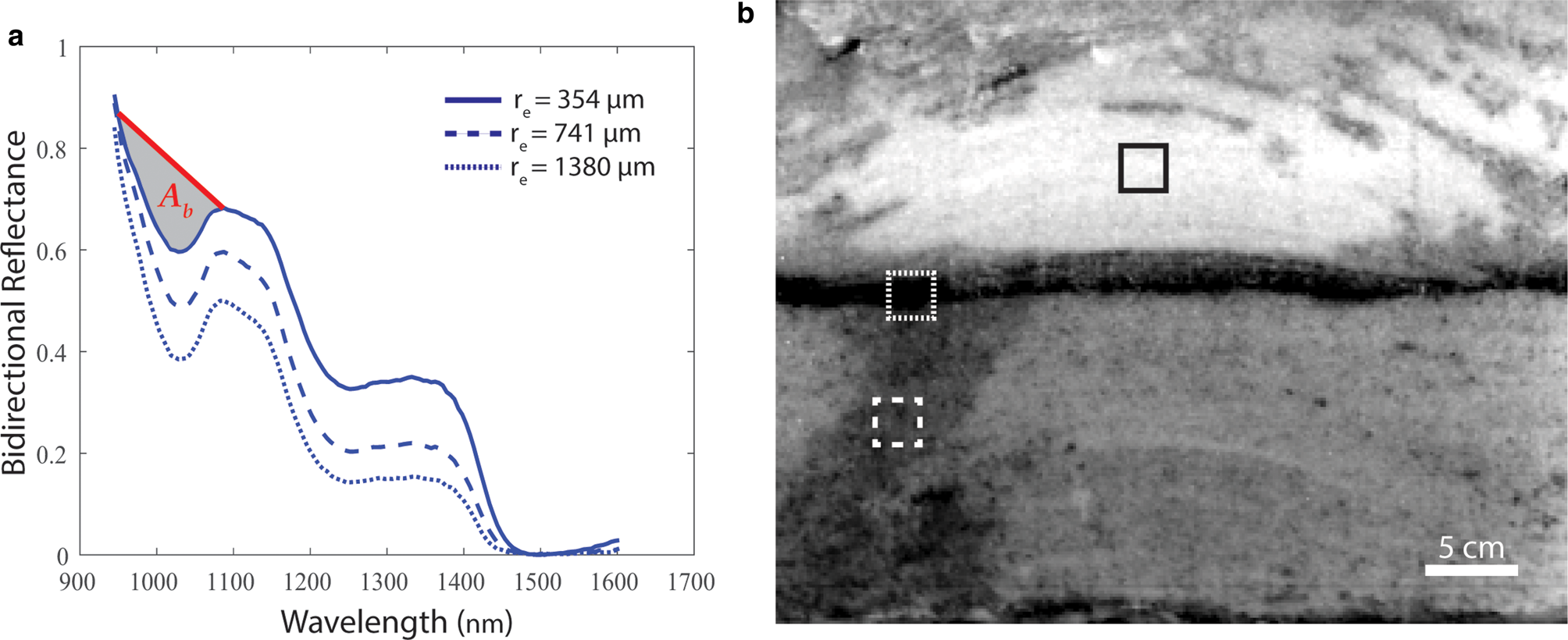
Fig. 2. (a) Three snow spectra are plotted from a single pixel located within the boxes of (b). For the solid line spectrum, an example of the scaled band area (A b) is shaded gray, which corresponds to an effective grain radius (r e) of 354 μm. The continuum reflectance, shown as the red line, is the slope between the shoulders of the ice absorption feature (λ = 984 nm and λ = 1087 nm). (b) Gray scale near-infrared image of the post-melt fine grain over coarse grains snow sample at λ = 1030 nm taken with the Resonon Pika NIR-320 hyperspectral imager. Each box represents an area with a different r e.
Nolin and Dozier (Reference Nolin and Dozier2000) validated their model with a crystal card, hand lens and stereology measurements, finding that retrieved r e matched measurements with a correlation coefficient of r = 0.997. They also assessed the sensitivity of the method to instrument noise, finding that retrieved r e between 30 and 900 μm could vary by ± 10–50 μm. The signal-to-noise ratio (SNR) used for AVIRIS in the study was 100, whereas the SNR for the Resonon Pika NIR-320 is 1885. With the better SNR and higher spectral resolution of the Pika NIR-320, the NIR-HSI method should be more robust with respect to sensor noise, when compared to the N-D method applied to AVIRIS.
In place of the Discrete Ordinates Radiative Transfer Program, or DISORT (Stamnes and others, Reference Stamnes, Tsay, Wiscombe and Jayaweera1988) used by N-D, the theoretical snow spectra in this study were modeled with the Snow, Ice, and Aerosol Radiative Transfer Model, or SNICAR (Flanner and others, Reference Flanner, Zender, Randerson and Rasch2007). SNICAR simulates radiative transfer through a snowpack comprised of spherical grains of ice at a given grain size and illumination geometry using the updated ice optical property compilation of Warren and Brandt (Reference Warren and Brandt2008). Model inputs include illumination angle, r e (μm), snow layer thickness (m), snow density (kg m−3) and when appropriate, concentrations of light-absorbing particles (ppb). In this case, we simulated snow directional-hemispherical reflectance for clean snow only, by running the model iteratively through r e values between 30 and 1500 μm. The other forcing inputs were held constant at values that best represent the bulk characteristics of the snow sample; 300 kg m−3 snow density, 0° illumination angle (light source perpendicular to snow surface) and a single optically thick snow layer. We did not vary the snow layer thickness because light penetration in the NIR is very shallow (0.5–3 cm) and grain size can be considered mostly homogeneous at this scale (Warren, Reference Warren1982; Nolin and Dozier, Reference Nolin and Dozier2000). We also did not vary snow density because density has little to no effect on snow reflectance (Bohren and Beschta, Reference Bohren and Beschta1979).
To help visualize the NIR hyperspectral image, a grayscale image at λ = 1030 nm is shown in Figure 2b. In each pixel, r e is determined through the best match to the theoretical scaled band area values contained within a lookup table (Supplementary Material Table S1), populated from modeled snow spectra using SNICAR. In Figure 2a, three snow spectrums are plotted from single pixels located within the boxes in Figure 2b, representing areas in the image with different r e. Smaller grains are highlighted with the solid line box in an area where there was no water percolation. Larger grains and ice are highlighted in the dotted line box where there was water pooling at the capillary barrier then refreezing. Medium-sized grains are highlighted in the dashed line box where there was a preferential flow path. For the solid line spectrum in Figure 2a, an example of the scaled band area (A b) is shown, which corresponded to r e = 354 μm using the lookup table.
2.3 Laboratory experiments
To demonstrate the novelty of the NIR-HSI method presented here, three laboratory-prepared snow samples with varying snow stratigraphy were analyzed initially and post-melt in the Subzero Research Laboratory (SRL) at Montana State University. The stratigraphy scenarios were homogeneous snow, a snow sample with an ice lens placed in the middle and a snow sample with fine grains sieved over coarse grains. In all cases, snow collected outside was sieved into a polystyrene box (42.5 cm × 42.5 cm × 38.1 cm) with a removable top and sidewall. The homogeneous snow sample was prepared by sifting snow using a 0.68 mm sieve. For the ice lens, snow grains were initially sifted using a 1.2 mm sieve, followed by fine misting water that had been chilled to 0 °C over the snow sample, such that it froze on contact creating an ice ‘lens’. Once the ice lens was completely frozen, the top layer of snow grains was sifted on top of the ice lens using the same 1.2 mm sieve. For the snow sample with fine grains placed over the top of coarse grains, the coarse grains at the bottom were sieved with a range of 1.5–5 mm, while the fine grains on top were sifted using a 1.2 mm sieve.
An initial hyperspectral image of each snow sample sidewall was taken to map r e prior to melt, under the assumption that the stratigraphy was approximately uniform throughout the snow sample. The snow samples were then placed under a metal-halide lamp that simulates the complete solar spectrum for ~6 h, while the room temperature was held constant at −5 ± 1 °C. The homogeneous snow sample was subjected to a simulated solar irradiance of 800 W m−2, while the ice lens and fine over coarse grain samples were subjected to a simulated solar irradiance of 650 W m−2. Once the solar lamp was turned off, the snow samples were moved to a separate storage chamber within the SRL and held at −30 °C for rapid refreezing. After 24 h at −30 °C, the sidewall of the polystyrene box was removed to reveal the snow stratigraphy, like viewing a snow pit wall in the field. Each snow sample sidewall was serial sectioned using a snow saw at intervals of 3–5 cm, with hyperspectral images taken of the sidewall between the removal of each section. Each image was processed using the methodology outlined above in Section 2.2 to map r e across each image. To illustrate this method, we present one imaged cross-section for each snow sample, initially and post-melt.
2.4 Method assessment
2.4.1 Instrument comparison
To assess the validity of the NIR-HSI method, the r e retrieval from the hyperspectral imager was compared to retrieval methods using a field spectrometer and micro-CT. A homogeneous snow sample (1 mm sieved snow grains) was prepared using the method described in Section 2.3 and the snow sample sidewall was measured with each instrument for comparison. The snow sample sidewall was first imaged with the hyperspectral imager, resulting in 54 570 spatial pixels, which was inverted to r e using the method described in Section 2.2.
Next, using the same halogen light source and white reference panel, sidewall reflectance was measured using an Analytical Spectral Devices (ASD) FieldSpec 4 High Resolution field spectrometer, which has a spectral range of 350–2500 nm, and spectral bandwidth of 1.1 nm in the NIR. To reduce shadowing, the halogen light source was positioned to the side of the spectrometer (15° off nadir). The field of view was reduced using an 8° fore optic, which was held perpendicular to the sidewall at a distance of ~4 cm from the snow surface, resulting in an approximate spot size of 5.6 mm. Following a white reference measurement, 30 discrete measurements of snow reflectance were made in a space covering a grid pattern. Each spectrum was then inverted for r e using the method described in Section 2.2 but using a separate lookup table for an illumination angle of 15°.
Last, five snow sub-samples were cut from the snow sample sidewall for measurement using a SkyScan 1173 micro-CT housed in a −10°C cold room in the SRL. Samples were measured in a 33 mm diameter × 67 mm long cylindrical tube that allowed for a voxel size of 19.4 μm. Measurements were taken using a 42 kV, 190 mA X-ray beam, 100 ms exposure time, and each sample was rotated 180° at 0.7° increments. The scanning time of each sample was ~25 min and all five samples were measured within 3 h of the hyperspectral imager and field spectrometer measurements. Additionally, a 3 × 3 × 3 median filter was applied to the reconstructed images, thresholding of the grey-scale images into ice and air phases was performed by visual inspection, and a despeckling filter was used to remove both white and black speckles <25 voxels. The volume and surface area of each snow sample was measured in 3D based on the marching cubes method (Lorensen and Cline, Reference Lorensen and Cline1987). The total surface area calculated from the proprietary Bruker micro-CT analysis software (CTAn) includes ‘false’ surface area from the volume of interest intersecting snow grains, which is believed to add a positive bias to the measured SSA. Conversely, removing the intersection surface area from the total surface area results in a negative bias to the measured SSA, whereas the actual SSA resides somewhere in the middle. Therefore, we report the average SSA value measured by including intersection surface area and removing intersection surface area to calculate r e using Eqn (1).
To quantitatively compare r e retrievals between each instrument, the mean, std dev. and distributions of r e were compared and visualized. Furthermore, each measurement from the micro-CT and field spectrometer was overlaid onto the r e map produced by the hyperspectral imager to visualize the spatial variability between all retrievals. These results are shown in Section 3.2.
2.4.2 Sensitivity to illumination angle
Because it is an important control on NIR reflectance, the NIR-HSI method relies on the illumination angle to be correctly accounted for when generating r e lookup tables. At higher incidence angles, a photon will, on average, undergo its first scattering event closer to the surface which increases the probability of scattering in an upward direction, exiting the snowpack without being absorbed (Warren, Reference Warren1982). Therefore, for the same r e, reflectance increases with illumination angle, resulting in smaller A b values. For example, Figure 3 shows the directional-hemispherical reflectance at 0°, 30° and 45° illumination angles for an r e of 100 μm modeled using SNICAR. In assessing the sensitivity of the retrieval of r e to illumination angle, we note that although for modeling purposes we assume the halogen lights are at 0°, there are slight variations from this in our experiments. This is due to two factors, (1) the two halogen lights can be independently rotated, and (2) the lights must be placed slightly below the scanning stage to not obstruct the field of view of the imager.
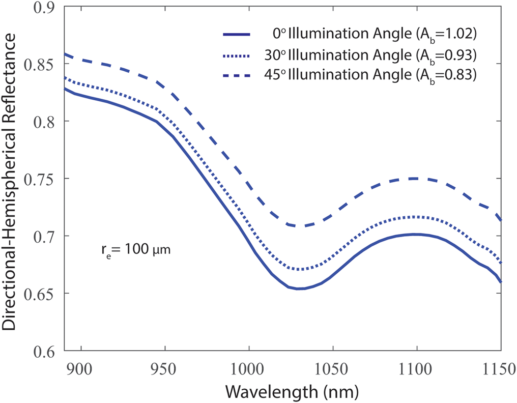
Fig. 3. Directional-hemispherical reflectance at 0°, 30° and 45° illumination angles for effective grain radius (r e) of 100 μm modeled using SNICAR. Scaled band area (A b) of the ice absorption feature centered at 1030 nm decreases with increasing illumination angle.
The sensitivity of the r e retrieval to variation in illumination angle was assessed by comparing consecutive images of the same homogeneous snow sample sidewall, prepared following the procedure in Section 2.2. While the hyperspectral imager remained stationary and perpendicular to the snow sample sidewall, the halogen lights were moved from 0° to 45° illumination angles at increments of 5°. To demonstrate the error that can result from not specifying the correct illumination angle, each image was processed using the lookup table for a 0° illumination angle and compared to additional lookup tables generated with SNICAR for the corresponding illumination angles.
2.4.3 Repeatability
Multiple images of a homogeneous snow sample were also used to assess sensitivity to sensor noise and investigate the precision of the r e retrieval. To accomplish this, the snow sample sidewall was imaged five consecutive times over a 3 min time period without any changes made to the experimental setup. To compare the consistency in r e retrievals, we compare the range of values from each image using a box plot analysis and assess spatial differences with pixel by pixel std dev. However, since it was not possible to exactly align pixels between images, std dev. were calculated over 3.5 cm2 subregions of the image. This represents the average std dev. across ~20 × 20 pixels in the original images.
3. Results and discussion
3.1 Laboratory experiment
In Figures 4a–f, r e is shown for the three laboratory-prepared snow samples initially and post-melt. Although the lookup table for these measurements is populated for grains with r e ranging from 30 to 1500 μm, to increase contrast and improve visualization, the color bar used in Figure 4 ranges from only 30 to 1000 μm. Grains outside the range of the lookup table are white (r e ⩾ 1500 μm) and classified as ice. In Figures 4g–i, the initial and post-melt r e distributions are plotted to show the shift in r e due to grain coarsening during wet snow metamorphism (Raymond and Tusima, Reference Raymond and Tusima1979). Interestingly, the r e maps reveal patterns in the stratigraphy profile, seen best in initial images Figures 4a–c, which are due to the laboratory sifting process. This is the first time, of which we are aware, that this pattern has been captured and shows that although still relatively homogeneous at the sample scale, the sifting process itself does introduce spatial variability.

Fig. 4. (a–c) Effective grain radius (r e) map for three laboratory-prepared snow samples; (a) homogeneous, (b) ice lens, (c) fine grains over coarse grains. (d–f) Post-melt r e map for the three initial snow samples shown in (a–c). (g–i) Distribution of r e for each snow sample initially, and post-melt.
Prior to melt, the homogeneous snow sample mean r e was 149 μm (std dev. (σ) = 17 μm), whereas the post-melt mean r e was 191 μm (σ = 53 μm) (Figs 4a, d). The sample was prepared in a way that classical grain size would be homogeneous throughout the sample, and the homogeneity was also present in the mapped r e, with the corresponding distribution being relatively narrow and unimodal (Fig. 4g). Post-melt, the r e increased and the distribution widened due to grain coarsening and wet snow metamorphism. This example demonstrates that this method can be used to quantify and map the magnitude of grain coarsening post-melt and visualize preferential flow channels in refrozen snow (Fig. 4g).
Initial mean r e for the snow sample containing an ice lens was 211 μm (σ = 41 μm), and the post-melt mean r e was 395 μm (σ = 148 μm) (Figs 4b, e). Like the homogeneous sample, the corresponding distribution (Fig. 4h) is unimodal, but with a broader r e range for both the initial and post-melt r e maps. In the initial image, it is evident that the shift in the distribution relative to the homogeneous sample is primarily due to the larger grains associated with the ice lens. In the post-melt image, r e has generally increased across the full image, and the r e map shows evidence of preferential flow channels and pooling water at the ice lens interface.
In the fine over coarse grain snow sample, the initial mean r e was 292 μm (σ = 110 μm), while the post-melt mean r e was 452 μm (σ = 192 μm) (Figs 4c, f). The layer of fine grains over coarse grains is clearly visualized in the initial and post-melt r e maps, and corresponding distributions (Fig. 4i), which were bimodal. In the post-melt image, evidence of water pooling at the interface between fine and coarse r e, referred to as a capillary barrier (Waldner and others, Reference Waldner, Schneebeli, Schultze-Zimmermann and Flühler2004), can be seen by the formation of an ice layer surrounded by larger grains. Capillary barriers in a snowpack are generally due to infiltrating water in finer grains having a very high suction, which prevents water from entering the lower (coarse grain) layer, causing local accumulation of water at the interface (ponding) and horizontal diversion of water (Yamaguchi and others, Reference Yamaguchi, Katsushima, Sato and Kumakura2010; Avanzi and others, Reference Avanzi, Hirashima, Yamaguchi, Katsushima and Michele2016).
As mentioned in Section 2.3, it should be noted that in all the hyperspectral images presented here, the snow samples had been refrozen at −30°C, such that there was no liquid water present (i.e. dry snow) during the data collection. This is important to reiterate because the presence of liquid water in snow does affect the ice absorption feature centered at 1030 nm due to the two absorption features associated with liquid water at 950 and 1150 nm (Nolin and Dozier, Reference Nolin and Dozier2000). Furthermore, Green and Dozier (Reference Green and Dozier1996) demonstrated that high amounts of liquid water (25% by volume) shifted the ice absorption feature to shorter wavelengths and reduced the depth. However, Nolin and Dozier (Reference Nolin and Dozier2000) reported that for low amounts of liquid water (3–5% by volume), there were no effects on the accuracy of the r e retrievals using the scaled band area (N-D) method.
3.2 Instrument comparison
The retrieved r e from each instrument is shown in a box plot analysis in Figure 5a. The mean r e, std dev. (σ), and number of samples (n) for the hyperspectral imager, field spectrometer and micro-CT, respectively, were: r e = 151 μm, (σ) = 20 μm, (n) = 54 570; r e = 151 μm, σ = 7 μm, n = 30; r e = 192 ± 2 μm, σ = 12 μm and n = 5. The mean r e value from the field spectrometer matched that of the hyperspectral imager, although the median value was 4% higher. Additionally, the full range of spectrometer r e values generally aligned with the interquartile range of the hyperspectral imager, but the full range was not represented in the distribution. The retrieved r e from the micro-CT fell within the upper range of r e values from the hyperspectral imager, but the mean r e was 23.9% higher.
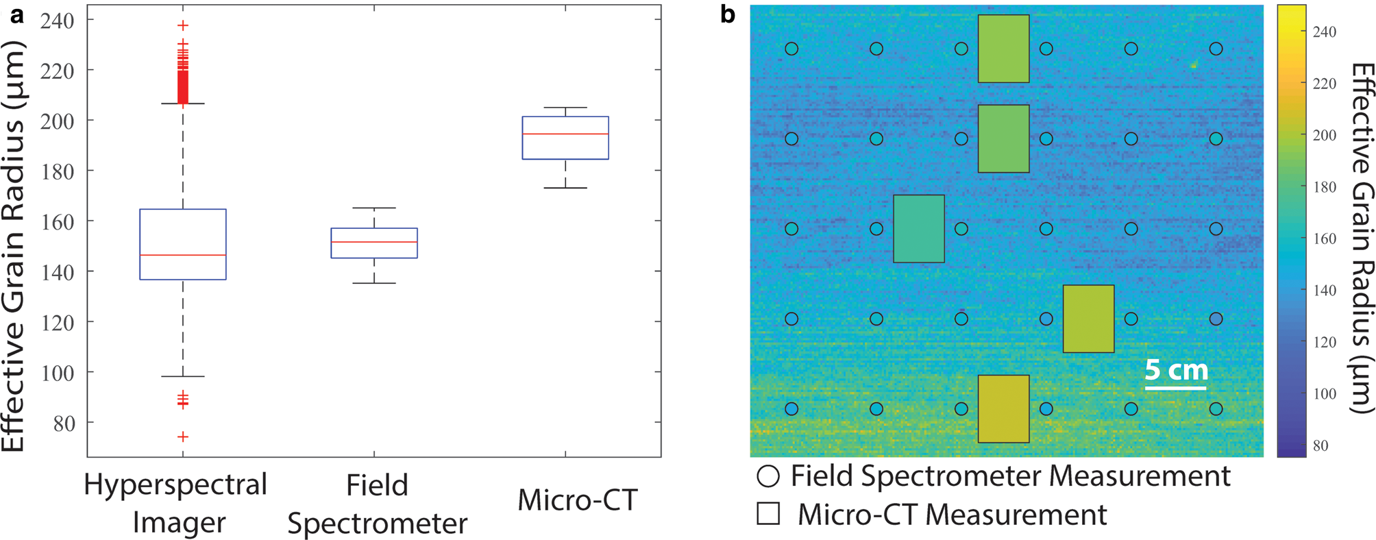
Fig. 5. Effective grain radius (r e) retrieval comparison between the hyperspectral imager, field spectrometer and micro-CT using a homogeneous snow sample. (a) Box plot showing the median, range and distribution of r e from each instrument. (b) Map of r e retrieved from the hyperspectral imager overlaid with field spectrometer and micro-CT measurements. The circles representing the field spectrometer have been enlarged for better visualization.
The map of r e retrievals from all three instruments is shown in Figure 5b. Although this snow sample was prepared to be homogeneous, the r e map revealed slightly larger grains at the top and bottom of the snow sample. This spatial variability was not seen in field spectrometer retrievals; however, it is important to note that the spot size (~5.6 mm) only spans a few pixels (~3 mm) and the circles representing these measurements were only enlarged for better visualization in the figure. The micro-CT r e measurements, which are shown approximately to scale, were higher relative to the other methods. The general trend, however, was captured across the vertical profile, as illustrated in Figure 5b.
It was expected that the r e retrievals between the hyperspectral imager and field spectrometer would be similar given that the N-D method was applied to both instruments. This close match in mean r e values demonstrates that the instrument specifications of the hyperspectral imager are sufficient to retrieve an accurate r e. Provided that the field spectrometer has a significantly higher spectral resolution, broader range and better SNR than the hyperspectral imager, this is an encouraging result. The spatial variability in r e values between the two instruments (Fig. 5b) is primarily attributed to the comparison design (i.e. fewer number of spectrometer measurements and difference in field of view), but also demonstrates the value of using a mapping technique for a more complete characterization of the r e range and spatial variability, as evidenced in Figure 5 for the hyperspectral imager.
The discrepancy in values between the hyperspectral imager and micro-CT could be attributed to multiple factors. First, there is a fundamental difference in measurement methods. The micro-CT measures the actual snow grain surface area and volume, which is converted to r e using the relationship in Eqn (1). Whereas the hyperspectral imager and field spectrometer are optically based methods that use a radiative transfer inversion technique based on snow grains modeled as spheres. It has been demonstrated that SSA from optical methods could have uncertainties by not accounting for grain shape (Picard and others, Reference Picard, Arnaud, Domine and Fily2009). Additionally, there are two experimental factors that could have contributed to the discrepancy in r e values; (1) the micro-CT measures a volume that extends 33 mm into the snow sample sidewall, whereas the hyperspectral imager and field spectrometer measure r e only at the snow surface, due to the shallow penetration of light in the NIR wavelengths, and (2) the five micro-CT scans spanned ~3 h post reflectance measurements, during which some change in the grain morphology may have occurred. These results are similar to reported values in Gergely and others (Reference Gergely, Wolfsperger and Schneebeli2014), where r e values retrieved from NIR reflectance measurements using the Infrasnow instrument were within 25% of micro-CT measurements. Although Nolin and Dozier (Reference Nolin and Dozier2000) report a much better agreement (r = 0.997) between retrieved r e and measured r e, we cannot compare these micro-CT results to those because they do not specify which of their measured grain radii are from stereology versus hand lens.
3.3 Sensitivity to illumination angle
The primary goal of the illumination sensitivity experiment was to assess how deviations in the light source illumination angle from nadir (0°) could impact the NIR-HSI method r e retrieval. As noted in Section 2.4.2, images were progressively collected across increasing illumination angles, and 0° was treated as the baseline against which all other retrievals were compared. The baseline image mean r e was 120 μm (red line in Fig. 6). When the 0° lookup table was used at all other angles the retrieved r e decreased relative to the baseline image, from 119 μm at 5° to 83 μm at 45°, with the decrease being relatively proportional to the cosine of the illumination angle (Fig. 6, squares and dashed blue line). For the r e retrievals presented in Section 3.1, we assumed the halogen light source was at a 0° ± 5° and processed images with a 0° illumination angle lookup table. The deviation of mean r e values was <1% between 0° and 5°, indicating that slight deviations from 0° do not significantly impact the r e retrieval, but that larger deviations would introduce a bias toward smaller r e (Fig. 6).
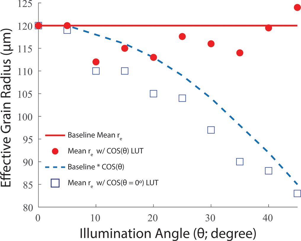
Fig. 6. Sensitivity of illumination angle to the effective grain radius (r e) retrieval method. Retrieved mean r e using the lookup table generated for nadir illumination (θ = 0°) is plotted as a function of illumination angle as blue squares. The decrease is relatively proportional to the baseline r e multiplied by the cosine of the illumination angle (dashed blue line). Mean r e retrievals using a lookup table generated with the correct illumination angle are plotted as red circles and compared to the baseline mean r e from nadir illumination (red line).
On the other hand, comparable mean r e values to the baseline image were retrieved across all illumination angles included in the experiment when individual lookup tables were generated for each respective illumination angle tested (Fig. 6, circles). The difference between mean r e at increasing illumination angles, relative to the baseline image, was 0 μm at 5° and then ranged from −8 μm at 10° to + 4 at 45°. Although the error between these results and the baseline data are within the repeatability range of this method, discussed further in Section 3.4, having an off-nadir illumination angle introduces angular uncertainties into the retrieval.
In the NIR wavelengths, snow reflectance is anisotropic, preferentially scattering light in the forward direction (Warren, Reference Warren1982). This can impact the accuracy of retrieving r e from measured directional reflectance (Painter and Dozier, Reference Painter and Dozier2004a, Reference Painter and Dozier2004b). When the illumination angle is nadir, however, snow reflectance is essentially Lambertian (Dumont and others, Reference Dumont2010). In our experimental setup, the uncertainty due to angular effects was minimized by keeping the view and illumination angles nadir. If both the view and illumination angles were off-nadir, using a radiative transfer model that computes angular intensities, like DISORT, would be recommended.
Lastly, we recognize that the lights used in these experiments introduce some level of uncertainty, even if minor, because the illumination may vary slightly between images. The method could be improved by modifying the light source to minimize slight variations in illumination angle. For example, lights could be fully diffused and/or co-aligned with the imager and evenly spaced around the lens. This would allow the lights to rotate with the imager, resulting in a better quasi-monostatic measurement.
3.4 Repeatability
The box plot analysis, shown in Figure 7a, shows that the general distribution of r e values is similar across all five consecutive images used to test repeatability. The interquartile range for each image spans ~20–30 μm, while the full range is ~110–220 μm. The mean r e ranged from 147 to 161 μm across the five images and was 151 μm for all images with a std dev. of 5 μm. Among all images, image 4 stands out as having a slight shift to higher values.

Fig. 7. Hyperspectral imager repeatability results to assess sensitivity to sensor noise. (a) Box plot analysis of five consecutively obtained images. (b) Histogram of the per pixel (3.5 cm2 subregion) std dev. of mean effective grain radius (r e) from the snow sample sidewall imaged, (c) map of r e standard deviations across the snow sample sidewall subregions.
To assess the spatial variability across repeated images, the std dev. of the mean r e was calculated in 3.5 cm2 subregions (20 × 20 pixels). The distribution of std dev. is shown in Figure 7b and a map of std dev. corresponding to the snow sample sidewall is shown in Figure 7c. The std dev. are randomly distributed across the image, indicating that the repeatability is most likely due to sensor noise, which can be approximated as Gaussian (Fig. 7b). The mean std dev. across subregions was 9 μm, which we use as the repeatability of the instrument. This repeatability is lower than the error due to sensor noise from AVIRIS bands (±10–50 μm) reported by Nolin and Dozier (Reference Nolin and Dozier2000), which can be attributed to the Resonon imager having more spectral bands across the ice absorption feature and a higher SNR.
4. Conclusion and future applications
We presented a new high spatial resolution NIR-HSI method to map r e from spectral reflectance data measured with a Resonon Pika NIR-320 compact hyperspectral imager. To demonstrate the effectiveness of the method over a wide range of r e, the method was applied to laboratory-prepared snow samples that had undergone wet snow metamorphism induced by a simulated solar lamp. Our results demonstrate that the NIR-HSI method can be a valuable tool for (1) quantifying spatial and temporal variability in r e, (2) measuring change in grain size, (3) investigating wet snow metamorphism under refrozen conditions and (4) visualizing liquid water flow in a refrozen snowpack.
Additionally, the NIR-HSI method was compared to r e retrievals from a field spectrometer and micro-CT. It was found that the hyperspectral imager r e retrieval compared well to the higher spectral resolution field spectrometer but was better able to capture spatial variability due to the extensive number of data points produced from the mapping technique. Although it was found that micro-CT mean r e values were 23.9% higher than that of the hyperspectral imager, the vertical profile followed the same spatial trend seen in the r e map produced by the NIR-HSI method.
This robust high-resolution mapping method fills a gap in current r e retrievals. There is increasing commercial availability of compact hyperspectral imagers, at feasible size and weight for laboratory and field applications, which will make this method more accessible. Although outside the scope of this paper, this method could be extended into the field to map r e in an excavated snow pit or at the surface when mounted on an unmanned aerial vehicle. For field applications, careful consideration of illumination conditions would be important for accurate r e retrievals. Mapping r e at the snow surface would require lookup tables to be generated for the solar zenith angle at the time of measurement. In a snow pit, mapping r e becomes more challenging because the direct and diffuse light ratio is unknown and would require some approximations to be made when generating the lookup table.
Supplementary material
The supplementary material for this article can be found at https://doi.org/10.1017/jog.2020.68
Acknowledgements
This research was supported by the NASA New Investigator Program Award 80NSSC18K0822. Additionally, Skiles was supported by the University of Utah GCSC, SWC, and Nexus. We acknowledge Resonon Inc. for supplying the hyperspectral imager used in this study. We also thank James Dillon and Ladean McKittrick for their assistance in the laboratory. We also acknowledge the use of the Subzero Research Laboratory in the Department of Civil Engineering at Montana State University. We thank Ghislain Picard and Henning Löwe for providing insightful comments that helped improve this manuscript. The presented data are available upon request from the lead author.


 Open access