


1. INTRODUCTION
Despite comprising a small fraction of the world's total ice volume, the majority of which is in the ice sheets of Greenland and Antarctica, mountain glaciers and ice caps are major contributors to ongoing sea-level rise (SLR). The glacier contribution to SLR is projected to be in the range 0.07–0.17 m by the end of the 21st century, which is roughly a third of the total projected SLR (Radić and Hock, Reference Radić and Hock2011). This can cause severe damage to small island states and coastal and low-lying areas (Wong and others, Reference Wong, Field, Barros, Dokken, Mach, Mastrandrea, Bilir, Chatterjee, Ebi, Estrada, Genova, Girma, Kissel, Levy, MacCracken, Mastrandrea and White2014). Routes for adaptation to climate change are highly reliant on accurate SLR projections, and thus such estimates are of high social importance (Lowe and Gregory, Reference Lowe and Gregory2010). On the regional and local scale, mountain glaciers affect water availability and retreating glaciers can cause geohazards.
Current approaches to projecting glacier mass or volume changes on regional and global scales rely on relatively simple models of glacier evolution (Marzeion and others, Reference Marzeion, Jarosch and Hofer2012; Radić and others, Reference Radić2014; Clarke and others, Reference Clarke, Jarosch, Anslow, Radić and Menounos2015; Huss and Hock, Reference Huss and Hock2015). More sophisticated models (e.g., Clarke and others, Reference Clarke, Jarosch, Anslow, Radić and Menounos2015) are difficult to apply at a global scale, both due to computational demands and the absence of sufficiently detailed input data (see also Huss and Fischer, Reference Huss and Fischer2016). Simple models of glacier evolution typically describe the glacier geometry using a small number of degrees of freedom (such as glacier length or thickness at certain locations, e.g., Roe and Baker, Reference Roe and Baker2014), and reduce their dynamics to a statement of mass balance combined with a set of heuristic or empirical closures that reflect the mechanics of glacier flow and feedbacks between glacier geometry and surface mass balance. Glacier volume is the primary output of these models and is computed from the dynamical degrees of freedom. A key challenge for these simplified glacier flow models is to represent the effects of bed geometry, which is often poorly known for individual glaciers, and of surface mass balance, for which detailed information only exists for a handful of glaciers with long-term monitoring programs.
In fact, fewer than 1% of glaciers worldwide have long-term mass-balance observations and detailed bedrock elevation data. All current models of regional glacier evolution apply statistical methods to extrapolate model parameters or results from glaciers with detailed observations to those without. These regional and global-scale projections, therefore, suffer from substantial uncertainties rooted in the statistical and/or scaling methods whose performance cannot be adequately validated (e.g., Radić and Hock, Reference Radić and Hock2014). This by itself makes the use of sophisticated three-dimensional glacier flow models questionable, even without accounting for the computational demands of such models.
A simplified approach to simulating glacier response to climate, therefore, remains useful. Using one such approach, Harrison (Reference Harrison2013) analyzed the most general properties of the response of valley glaciers to climate perturbations, aiming to improve methods for simulating glaciers with incomplete or underresolved data. While the model was designed to simulate glacier response to climate perturbation, the model itself has not been applied or tested on a real glacier. The goal of this study, therefore, is to apply an improved version of Harrison's model to real glaciers worldwide in order to analyze the regional sensitivity of glaciers to climate change. To improve the original model, we incorporate a better description of glacier flow and glacier geometry, and of the feedback between geometry and surface mass balance. We focus our discussion on the attribution of variability in glacier sensitivities to temperature perturbations and their response times, aiming to distinguish factors related to glacier and bedrock geometry from factors determined by climatic setting.
2. MODEL
In Harrison's original model of glacier evolution, a glacier is simulated as a block of ice with a length L, time-independent uniform width W and time-independent uniform height H (Fig. 1). A mass-balance rate distribution with height,  $\dot {b}$, is specified as a linear function of elevation, z. Integrating $\dot {b}$ over the glacier surface gives the glacier-wide mass-balance rate $\dot {B}$. In this study, we extend the block model using volume–length and volume–area scaling instead of keeping the time-independent width and thickness. We also use a mass-balance rate gradient for the ablation area, $\dot {g}_{{\rm abl}}$, that differs from the gradient for the accumulation area, $\dot {g}_{{\rm acc}}$, as opposed to a single gradient over the entire glacier. The mass-balance profiles of many glaciers are well approximated with piecewise-linear functions (Cuffey and Paterson, Reference Cuffey and Paterson2010); thus, introducing the separate mass-balance gradients in the model increases the versatility in representing real mass-balance profiles. As we will show later, having two different gradients also overcomes a limitation of Harrison's model, namely that the accumulation area ratio (AAR) at equilibrium could only be 0.5.
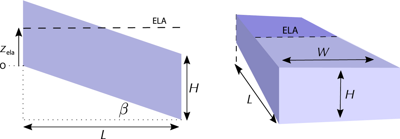
Fig. 1. Cross-section (left) and head-on (right) view of the block model with glacier length L, width W, height H, equilibrium line altitude  $z_{{\rm ela}}$ and surface slope β.
We define the mass-balance rate profile as
 $$\eqalign{ \dot b(z) & = \;{\dot g}_{{\rm abl}}(z - z_{{\rm ela}})\theta (z_{{\rm ela}} - z)\theta (z_{{\rm ela}} - (H - \beta L)) \cr & \quad + {\dot g}_{{\rm acc}}(z - z_{{\rm ela}})\theta (z - z_{{\rm ela}})\theta (H - z_{{\rm ela}}),} $$
where θ is the Heaviside step function (0 when the argument is negative, 1 when it is positive) and  $z_{{\rm ela}}$ is the height of the equilibrium line altitude (ELA) above the highest point on the glacier bed (point O in Fig. 1). In the case that there is both an ablation and accumulation area ( $H - \beta L \lt z_{\rm ela} \lt H$), $\dot {b}$ reduces to
 $$\dot b(z) = \left\{ \matrix{{\dot g}_{{\rm acc}}(z - z_{{\rm ela}}) \, {\rm for } \; z \gt z_{{\rm ela}}, \hfill \cr {\dot g}_{{\rm abl}}(z - z_{{\rm ela}}) \; {\rm for } \; z \lt z_{{\rm ela}}. \hfill} \right.$$
 As in Harrison's model, we assume that the bed has a constant downward slope β (note that β is the ratio of the vertical extent of the glacier below O to L, not the angle of inclination, which is given by  $\tan ^{-1} \beta $). If x is the horizontal distance down-glacier from point O, we have $z(x) = H - \beta x$ along the surface. Integrating the surface mass-balance rate $\dot {b}$ over the glacier surface gives the total rate of change of glacier volume with respect to time. Using ${\rm d}A = W{\rm d}x$ to compute that integral, we get
 $$\eqalign{ \displaystyle{{{\rm d}V} \over {{\rm d}t}} & = \int_0^L {\dot b} (z(x)){\mkern 1mu} W{\mkern 1mu} {\rm d}x \cr & = \left\{ \matrix{\bigg[\left( {{\dot g}_{{\rm acc}} - {\dot g}_{{\rm abl}}} \right)\displaystyle{{{(H - z_{{\rm ela}})}^2} \over {2\beta }}W \hfill \cr \quad+ {\dot g}_{{\rm abl}}\left( {(H - z_{{\rm ela}})WL - \beta W\displaystyle{{L^2} \over 2}} \right)\bigg ] \hfill \cr \; \; {\rm for } \; H - \beta L \lt z_{{\rm ela}} \lt H, \hfill \cr {\dot g}_{{\rm abl}}\left( {(H - z_{{\rm ela}})WL - \beta W\displaystyle{{L^2} \over 2}} \right)\; {\rm for } \; z_{{\rm ela}} \gt H, \hfill \cr {\dot g}_{{\rm acc}}\left( {(H - z_{{\rm ela}})WL - \beta W\displaystyle{{L^2} \over 2}} \right) \; {\rm for } \; z_{{\rm ela}} \lt H - \beta L. \hfill} \right.} $$
In Harrison's original model, changes in net mass balance are translated into changes in the terminus position, and thus length (and volume) is the only time-dependent geometric quantity. We add volume–length and volume–area scaling to capture the dependencies between length, height and width:
 $$ V = c_l L^p, \quad V = c_a A^\gamma, $$
where  $c_l$ and $c_a$ are glacier-specific constants, while p and γ are the universal scaling exponents (Bahr and others, Reference Bahr, Meier and Peckham1997). Following Bahr and others (Reference Bahr, Pfeffer and Kaser2015), for a linear mass-balance profile the appropriate γ value is 1.25, which we use in the numerical results below. This value of γ is within the range of expected physically reasonable values of $7/6 \leq \gamma \leq 3/2$. In the derivation of the equations, however, we leave γ unspecified. Using $p = \gamma /(2 - \gamma )$ from Bahr and others (Reference Bahr, Pfeffer and Kaser2015), we can now write the three dimensions in terms of the volume:
 $$\eqalign{H & = c_a^{1/\gamma } V^{(\gamma - 1)/\gamma }, \cr W & = c_a^{ - 1/\gamma } c_l^{(2 - \gamma )/\gamma } V^{(\gamma - 1)/\gamma }, \cr L & = c_l^{ - (2 - \gamma )/\gamma } V^{(2 - \gamma )/\gamma }.} $$
 Note that we have reduced the dynamics of the glacier to a single ordinary differential equation for volume (obtained by substituting Eqn (5) into (3); we omit for brevity). Our reduction to a single degree of freedom amounts to saying that the shape of the glacier adjusts instantaneously to changes in length, rather than requiring a finite amount of time as mass is redistributed along the glacier. The same instantaneous adjustment of glacier shape occurs in models that treat glaciers as perfectly plastic (Nye, Reference Nye1951), equivalent to taking  $n \to \infty $ in Glen's law (Cuffey and Paterson, Reference Cuffey and Paterson2010). We will discuss the implications on the glacier response later in the paper.
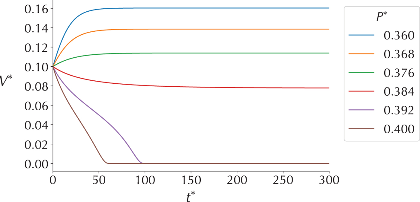
Fig. 2. Examples of volume evolution in time for  $G^{\ast} = 0$ and different values of $P^{\ast}$.
Next, we render the model in dimensionless form. This has the advantage of reducing the number of parameters in the model to a minimum. A length scale  $L_0$ can be defined through
 $$L_0 = \left( {\displaystyle{{2c_a^{1/\gamma } c_l^{(2 - \gamma )/\gamma } } \over \beta }} \right)^{ - \gamma /(6\gamma - 9)},$$
while the natural timescale for the problem is  $t_0 = 1/\dot {g}_{{\rm abl}}$ (later we will show that the e-folding time is a multiple of $t_0$). We find that typical values of $L_0$ fall between 10 and 100 m, and $t_0$ between 80 and 240 years. Using these, we can define a dimensionless time and volume through
 $$t^{\ast} = t/t_0,\quad V^{\ast} = V/L_0^3 .$$
In addition, we obtain two dimensionless parameters
 $$\eqalign{& G^{\ast} = \displaystyle{{{\dot g}_{{\rm acc}}} \over {{\dot g}_{{\rm abl}}}} - 1, \cr & P^{\ast} = z_{{\rm ela}}\left( {\displaystyle{{\beta ^{\gamma - 1}} \over {2^{\gamma - 1}{\mkern 1mu} c_a^{(2 - \gamma )/\gamma } {\mkern 1mu} c_l^{(2 - \gamma )(\gamma - 1)/\gamma } }}} \right)^{1/(3 - 2\gamma )}.} $$ $G^{\ast}$ is related to the mass-balance ratio or area-altitude balance ratio (AABR), $\dot {g}_{{\rm abl}}/\dot {g}_{{\rm acc}}$, a commonly used quantity in paleo-glacier reconstructions (Rea, Reference Rea2009), while $P^{\ast}$ is a dimensionless ELA. With the above change of variables, the model (Eqn (3)) becomes
 $$\displaystyle{{\rm d}V^{\ast} \over {\rm d}t^{\ast}} = \left\{\matrix{\bigg[\displaystyle{{G^{\ast}} \over 4}\left({V^{\ast}}^{(\gamma - 1)/\gamma} - P^{\ast}\right)^2{V^{\ast}}^{(\gamma - 1)/\gamma} - P^{\ast}{V^{\ast}}^{1/\gamma} \hfill \cr \quad - {V^{\ast}}^{(3 - \gamma)/\gamma} + V^{\ast} \bigg] \hfill \cr \; \; \hbox{for} -2\, {V^{\ast}}^{(2 - \gamma)/\gamma} \lt \left(P^{\ast} - {V^{\ast}}^{(\gamma - 1)/\gamma}\right) \lt 0,\hfill \cr \left[(G^{\ast} + 1)\left(-P^{\ast}{V^{\ast}}^{1/\gamma} - {V^{\ast}}^{(3 - \gamma)/\gamma} + V^{\ast}\right)\right] \hfill \cr \; \; \hbox{for} -2 {V^{\ast}}^{(2 - \gamma)/\gamma} + {V^{\ast}}^{(\gamma - 1)/\gamma} \gt P^{\ast},\hfill \cr \left[-P^{\ast}{V^{\ast}}^{1/\gamma} - {V^{\ast}}^{(3 - \gamma)/\gamma} + V^{\ast} \right]\hfill \cr \; \;\hbox{for} {V^{\ast}}^{(\gamma - 1)/\gamma} \lt P^{\ast}. \hfill}\right.$$
2.1. Equilibria, response times and bifurcation
Next, we analyze the model, focusing on steady states, their stability and sensitivity to parameter changes. Focusing on the properties of steady states means we do not capture the detail of how general, transient glacier evolution is affected by changes in climate forcing: the specific detail of these transients is dependent on the detail of how (and how fast) climatic forcing is changing compared with adjustments in glacier geometry and leads to little generic insight. Focusing on steady states allows us to define sensitivity to changes in climate and response times in a robust way, and captures the effect of low-frequency changes in climate, for which glaciers can be treated as being in pseudo-equilibrium (Roe, Reference Roe2011).
We now find the equilibria for the non-dimensionalized model as a function of  $G^{\ast}$ and $P^{\ast}$. Let $F(V^{\ast},\,G^{\ast},\,P^{\ast})$ be the right-hand side of Eqn (9). For a given set of parameters, steady-state solutions satisfy $F(V^{\ast},\,G^{\ast},\,P^{\ast}) = 0$; where such solutions exist, this defines a steady-state glacier volume as a function of the parameters $G^{\ast}$ and $P^{\ast}$, $V^{\ast} = V_s^{\ast}(G^{\ast},\,P^{\ast})$. $V_s^{\ast}$ is smooth except where $\partial F(V_s^{\ast},\,G^{\ast},\,P^{\ast})/\partial V^{\ast} = 0$. Non-zero equilibria in the model only exists for $G^{\ast} \gt -1$; this is always satisfied as $\dot {g}_{\rm acc}$ and $\dot {g}_{\rm abl}$ are positive by construction. With the procedure described in Appendix A, we can compute the steady-state volumes $V_s^{\ast}$ numerically for any given $G^{\ast}$ and $P^{\ast}$.
Next, we will define a response time by introducing a small perturbation to a steady-state glacier. If the glacier returns to a steady state after the perturbation is introduced, the steady state is considered to be stable. Take a steady state and perturb it slightly as  $V^{\ast} = V_s^{\ast}(G^{\ast},\,P^{\ast}) + \delta V^{\ast}$. Expanding in a two-term Taylor expansion, ${\rm d}V^{\ast}/{\rm d}t^{\ast} = F(V^{\ast}, G^{\ast}, P^{\ast}) \approx F(V_s^{\ast}, G^{\ast}, P^{\ast}) + \partial F/\partial V^{\ast}\vert _{V_s^{\ast} ,G^{\ast},P^{\ast}}\delta V^{\ast} = \partial F/\partial V^{\ast} \vert_{V_s^{\ast},G^{\ast},P^{\ast}}\delta V^{\ast}$, we obtain a linear equation for $\delta V$, with solution
 $$\delta V^{\ast} = \delta V^{\ast}(0)\exp \left[ {\displaystyle{{\partial F} \over {\partial V^{\ast}}}\left\vert {_{V_{_s }^{\ast} (G^{\ast},P^{\ast}),G^{\ast},P^{\ast}} t^{\ast}} \right.} \right].$$
The steady-state solution is stable if  $\delta V^{\ast}$ shrinks, that is, if the partial derivative $\partial F/\partial V^{\ast}$ is negative.
The e-folding time for the decay of  $\delta V^{\ast}$ is a robust measure for ‘response time’ to a given (small) perturbation. In dimensional time, that response time becomes
 $$\eqalign{ \tau &= - \left(\dot{g}_{\rm abl} \left. \displaystyle{\partial F \over \partial V^{\ast}} \right\vert_{V_s^{\ast} (G^{\ast}, P^{\ast}), G^{\ast}, P^{\ast}} \right)^{ - 1} \cr & = \left( - \displaystyle{G^{\ast} \over 4} \left( \displaystyle{\gamma - 1 \over \gamma} \right) \left(P^{\ast} - V_s^{* (\gamma - 1)/\gamma} \right)^2 V_s^{* - 1/\gamma} \right. \cr &\qquad + \displaystyle{G^{\ast} \over 2} \left( \displaystyle{\gamma - 1 \over \gamma} \right)\left(P^{\ast} - V_s^{* (\gamma - 1)/\gamma} \right) V_s^{* - (2 - \gamma )/\gamma} \cr &\qquad + \left(\displaystyle{3 - \gamma \over \gamma} \right) V_s^{* (3 - 2\gamma )/\gamma } \cr &\qquad \hskip 2.4pt \left. + \displaystyle{1 \over \gamma} P^{\ast} V_s^{* - (\gamma - 1)/\gamma} - 1 \right)^{ - 1} \dot{g}_{\rm abl}^{ - 1} .}$$
 This is related to the Harrison (Reference Harrison2013) volume response time  $\tau _V$, which can be written in our model as
 $$\eqalign{ \tau _V & = \left( {\displaystyle{{ - {\dot b}_t} \over H} - \dot g} \right)^{ - 1} \cr & = \left( {2{\mkern 1mu} V{_s^{\ast} }^{(3 - 2\gamma )/\gamma } + P^{\ast}V{_s^{\ast} }^{ - (\gamma - 1)/\gamma } - 1} \right)^{ - 1}{\dot g}_{{\rm abl}}^{ - 1} } $$
by noticing that the balance rate at the terminus  $\dot {b}_t = \dot {g}_{\rm abl}(-\beta L - z_{\rm ela})$. Equation (12) is equal to Eqn (11) when $G^{\ast} = 0$ ( $\dot {g}_{\rm abl} = \dot {g}_{\rm acc}$) and $\gamma = 1$ (which implies a constant height). Therefore Eqn (11) can be seen as a generalization of the volume response time of Harrison (Reference Harrison2013) (and is similar to $\tau _V = -H/\dot {b}_t$ as in Jóhannesson and others, Reference Jóhannesson, Raymond and Waddington1989), allowing for different mass-balance gradients in the ablation and accumulation area, and accounting for volume scaling.
There is a positive feedback between glacier thickness and mass balance, known as the altitude/mass-balance feedback (Cuffey and Paterson, Reference Cuffey and Paterson2010): a thicker glacier leads to a higher glacier surface, which generally leads to more accumulation and less ablation, i.e., more positive mass balance and vice-versa. This gives rise to a bifurcation, with  $P^{\ast}$ the bifurcation parameter (related to the ELA through Eqn (8)). When the ELA is located above the highest point on the glacier bed $P^{\ast} = 0$, but lower than a critical value $P^{\ast} = P_0^{\ast}$, the model is bistable (Fig. 3, center). Removing the glacier leaves a stable zero-volume solution, while for ELAs that are not too far above the highest point on the glacier bed, an existing glacier may still have a high enough surface to have a sufficiently large surface mass balance to persist stably. For ELAs below the highest point on the glacier bed, a glacier has to exist and there is a single stable steady state (Fig. 3, right). The bifurcation is a robust feature of other glacier flow models (Oerlemans, Reference Oerlemans2008; Giesen, Reference Giesen2009), but is absent from the original Harrison model because the latter treats ice thickness as prescribed. Figure 2 shows some example model trajectories, before and after the bifurcation point.
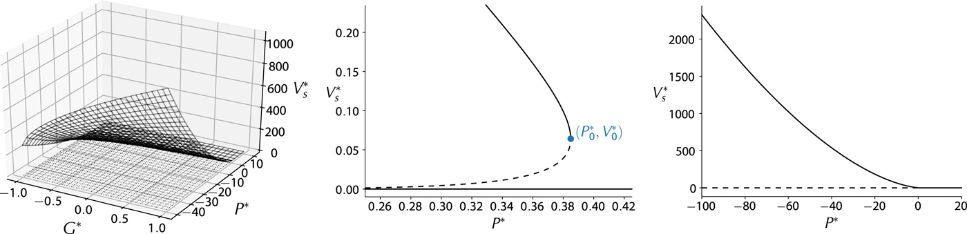
Fig. 3. Left: bifurcation diagram of  $V_s^{\ast}$ in $P^{\ast}$ and $G^{\ast}$. Center: bifurcation diagram for $G^{\ast}=0$ near the bifurcation point $P_0^{\ast}$. Right: same as center panel but for a wider range of $P^{\ast}$. Dotted lines indicate unstable equilibria, solid lines stable.
By setting  $F(V^{\ast},\, G^{\ast},\, P^{\ast}) = 0$, we can solve for $P^{\ast}$ in terms of $V^{\ast}$ at steady state. Noting that at the bifurcation point $(P_0^{\ast}$, $ V_0^{\ast}$), ${\rm d} P^{\ast}/{\rm d} V_s^{\ast} = 0$, this gives us the location of the bifurcation point for general $G^{\ast}$:
 $$\eqalign{& P_0^{\ast} = \left( {\displaystyle{{3 - 2\gamma } \over {2 - \gamma }}} \right)\left( {\displaystyle{{G^{\ast}(\gamma - 1)} \over {2\left( {\sqrt {G^{\ast} + 1} - 1} \right)(2 - \gamma )}}} \right)^{(\gamma - 1)/(3 - 2\gamma )}, \cr & V_0^{\ast} = \left( {\displaystyle{{G^{\ast}(\gamma - 1)} \over {2\left( {\sqrt {G^{\ast} + 1} - 1} \right)(2 - \gamma )}}} \right)^{\gamma /(3 - 2\gamma )}.} $$ $V_0 = L_0^3V_0^{\ast}$ is the minimum stable volume for a given glacier.
2.2. Accumulation area ratio
The AAR of a glacier is defined as the ratio of the area of the glacier with  $z \gt z_{\rm ela}$ to the area with $z \lt z_{\rm ela}$. AAR is often easier to infer, for instance from satellite measurements, than the actual mass-balance rates. Our version of Harrison's model predicts AAR as a simple function of the model parameter $G^{\ast}$; the calculation also shows why a single mass-balance gradient $\dot {g}_{\rm acc} = \dot {g}_{\rm abl}$ is inconsistent with frequently observed AAR values.
From the model geometry, we can determine the AAR to be
 $${\rm AAR} = \displaystyle{{H - z_{{\rm ela}}} \over {\beta L}}.$$
We set Eqn (3) to zero, solve for the steady-state length, and substitute into Eqn (14). This gives the steady-state AAR,
 $${\rm AA}{\rm R}_s = \displaystyle{1 \over {1 + \sqrt {G^{\ast} + 1} }}.$$
 According to Eqn (15), assuming a single mass-balance gradient (corresponding to  $G^{\ast}=0$) only allows for a steady-state AAR of 0.5, inconsistent with observed AARs which are typically ~0.6 for ‘healthy’ glaciers (Bahr and others, Reference Bahr, Meier and Peckham1997; Mernild and others, Reference Mernild, Lipscomb, Bahr, Radić and Zemp2013). An AAR of 0.6 corresponds to $G^{\ast}\simeq -0.56$.
2.3. Sensitivity to ELA changes
The original, dimensional model (Eqn (3)) contains three parameters characterizing climatic setting:  $\dot {g}_{\rm acc}$, $\dot {g}_{\rm abl}$ and $z_{\rm ela}$. We assume that local temperature affects only $z_{\rm ela}$ and leaves the $\dot {g}$ parameters unchanged. A simple measure of how much a change in temperature affects glaciers is the sensitivity of steady-state glacier volumes to changes in temperature, or equally, to $z_{\rm ela}$.
The dimensional sensitivity of volume to ELA is
 $$\displaystyle{{{\rm d}V_s} \over {{\rm d}z_{{\rm ela}}}} = L_0^3 \;\displaystyle{{\partial V_s^{\ast} } \over {\partial P^{\ast}}}\displaystyle{{{\rm d}P^{\ast}} \over {{\rm d}z_{{\rm ela}}}} = \left( {\displaystyle{{2{\mkern 1mu} c_l^{(2 - \gamma )/\gamma } } \over {\beta {\mkern 1mu} c_a^{2(\gamma - 1)/\gamma } }}} \right)^{1/(3 - 2\gamma )}\displaystyle{{\partial V_s^{\ast} } \over {\partial P^{\ast}}},$$
where
 $$\eqalign{ \displaystyle{{\partial V_s^{\ast} } \over {\partial P^{\ast}}} & = 1 \bigg / \displaystyle{{\partial P^{\ast}} \over {\partial V_s^{\ast} }} \cr & = \displaystyle{{\gamma {\mkern 1mu} G^{\ast}V{_s^{\ast} }^{(2\gamma + 1)/\gamma }} \over {2(\gamma - 2)\left( {\sqrt {G^{\ast} + 1} - 1} \right)V{_s^{\ast} }^{3/\gamma } + (\gamma - 1)G^{\ast}V{_s^{\ast} }^2}}.} $$
Note that the sensitivity is only meaningful for stable  $V_s^{\ast}$ ( $V_s^{\ast} \gt V_0^{\ast}$; see Eqn (13)). It is easy to verify that for $V_s^{\ast} \gt V_0^{\ast}$, ${\rm d} V_s^{\ast}/{\rm d} P^{\ast} \lt 0$, and steady-state volume decreases with increasing $z_{\rm ela}$ as expected.
Applying Eqn (16) to each glacier in a region, we quantify the relative regional glacier sensitivity to ELA perturbations by summing up all the individual glacier sensitivities per region and then normalizing by the total equilibrium volume of the region. The regional sensitivity for region r is thus
 $$\Sigma _r = \displaystyle{1 \over {\sum_{i} {{(V_s)}_i} }}\sum\limits_j {{\left( { - \displaystyle{{{\rm d}V_s} \over {{\rm d}z_{{\rm ela}}}}} \right)}_j} ,$$
where the sums are taken over all the glaciers in the region. The regional sensitivity can be viewed as an estimate of the fraction of the total equilibrium volume which would be lost if the ELA were increased by a unit distance for all glaciers in that region. However, the sensitivity is a derivative and thus inherently relevant to small perturbations, and is not able to capture the non-linearity of the model (e.g., the effect of increasing the ELA past the bifurcation point).
2.4. ELA distance
We define the following metric for how close glaciers in each region r are, in an aggregate sense, to the bifurcation that marks their ultimate disappearance. The sums are taken over all the glaciers in the region.
 $$d_r = \sum\limits_j {\displaystyle{{{(V_s)}_j} \over {\sum \nolimits_i {{(V_s)}_i} }}} \left( {\displaystyle{{{\rm d}z_{{\rm ela}}} \over {{\rm d}P^{\ast}}}} \right)_j(P_0^{\ast} (G_j^{\ast} ) - P_j^{\ast} ).$$
In the intercomparison among regions, a smaller value of  $d_r$ indicates that the glaciers in the region are closer to their disappearance point. $d_r$ is a sum of the inverse distances of each glacier's $P_j^{\ast}$ parameter from its bifurcation point $P^{\ast}_0(G_j^{\ast})$ (Eqn (13)), weighted by its fraction of the regional volume $(V_s)_j/\sum _i (V_s)_i$, and the extent to which a change in $P^{\ast}$ changes the ELA, measured by $({\rm d}z_{\rm ela}/{\rm d}P^{\ast})_j$. The latter factor is a unit conversion (see Eqn (8)) included because the distances $P^{\ast}_0(G_j^{\ast}) - P_j^{\ast}$, being non-dimensional, correspond to different ELA differences for each glacier. This metric should be interpreted with caution: as real glaciers retreat into higher altitudes, their slopes may change considerably, while our model assumes constant slope for each glacier.
3. MODEL APPLICATION ON GLACIERS WORLDWIDE
In this section, we apply the model to estimate the volume sensitivity to ELA perturbations and the response times for each glacier in the world glacier inventory dataset. Details about the data sources and methods are outlined below.
3.1. Glacier geometry data
We use the Randolph Glacier Inventory (RGI, version 5.0) (Pfeffer and others, Reference Pfeffer2014), containing information on glacier classification, location and basic geometry data. Because thickness and volume data are not included in the RGI, we use thickness estimates updated from Huss and Farinotti (Reference Huss and Farinotti2012) (Matthias Huss, personal communication). The updated data from Huss and Farinotti (Reference Huss and Farinotti2012) also includes glacier area and length data, which differ slightly from the RGI 5.0 values due to differences between the DEMs used by the RGI contributors and Huss and Farinotti. For consistency with the volume data source, therefore, we use the volume, area and slope from Huss and Farinotti (Reference Huss and Farinotti2012). We estimate lengths as  $L = (z_{\rm max} - z_{\rm min} - H)/\beta $, as per the block geometry (Fig. 1), where $z_{\rm max}$ and $z_{\rm min}$ are the maximum and minimum elevations of the glacier. The constants $c_l$ and $c_a$ that relate glacier volume to area and length depend on the shape of the valley occupied by the glacier, and cannot be taken as universal (Bahr and others, Reference Bahr, Pfeffer and Kaser2015). We estimate the constants' values for each glacier individually, using the initial volume, area and length as $c_l = V/L^p$ and $c_a = V/A^\gamma $ and keep the constants fixed in time. For glaciers with missing thickness values, we estimate these using a power law obtained from performing a linear least squares fit of $\log (V)$ to $\log (A)$ for glaciers with volumes in Huss and Farinotti (Reference Huss and Farinotti2012). As we describe later, we account for the uncertainties in the area, volume and thickness, and propagate these uncertainties to $c_l$ and $c_a$.
We exclude tidewater glaciers in our study because they can lose mass through calving and submarine melting, processes that are not incorporated in our model. We also exclude all ice caps, which behave differently from mountain glaciers in terms of volume–area/volume–length scaling and whose flow is also not driven predominantly by a non-zero bed slope β. Lastly, we exclude glaciers with missing surface slope information and those which have a reported altitude range smaller than their estimated thickness. In total, we apply the model to 91% of glaciers from RGI 5.0, comprising 34% of the RGI total glacier area (Table 1). Without the ice caps and tidewater glaciers, the modeled glaciers in some glacierized regions represent only a small fraction of the regional glacier area. For instance, <10% of the RGI glacier area is modeled for Iceland, the Russian Arctic and the Antarctic and Subantarctic region; see Table 1.
Table 1. Characteristics per RGI region: number and total area of modeled glaciers, percent of glaciers and their total area used from RGI 5.0

For each of the 19 RGI regions we provide an overview of regional estimates (mean and standard deviation) for the input variables used in the glacier evolution model: V, β,  $c_a$, $c_l$, $\dot {g}_{\rm abl}$ and $G^{\ast}$ (Table 2). Russian Arctic, Svalbard and Arctic Canada (North) have the largest mean volumes and also the smallest slopes. $c_l$ is highly correlated to the volume and thus the regional means of $c_l$ correspond in ranking to those of the volume.
Table 2. For each RGI region: mean ± standard deviation of model inputs. V ,  $c_a$ and $c_l$ are in units of m3, m $^{1/2}$ and m $^{4/3}$, respectively. $\dot {g}_{\rm abl}$ is given here in w.e. units.

3.2. ELA and mass-balance gradients
In order to estimate the sensitivities and response times, we need glacier-specific values for  $z_{{\rm ela}}$ and accumulation and ablation mass-balance gradients ( $\dot {g}_{\rm acc}$ and $\dot {g}_{\rm abl}$). Since the ELA is not known for the majority of glaciers in the RGI, various methods for ELA approximation have been proposed (Braithwaite and Raper, Reference Braithwaite and Raper2009; Braithwaite, Reference Braithwaite2015). These methods attempt to approximate the ‘balanced-budget’ ELA, and work well for glaciers near equilibrium. Since these methods rely on different mass-balance assumptions than our model (namely, a non-uniform hypsometry but a single mass-balance gradient), we instead estimate the ELA for each glacier as the ELA for which the glacier is in a steady state in our model. This amounts to setting
 $$P^{\ast} = \displaystyle{{{G^{\ast}}{V^{\ast}}{^2} - 2{\mkern 1mu} {V^{\ast}}^{3/\gamma } \left( {\sqrt {G^{\ast} + 1} - 1} \right)} \over {{G^{\ast}}{V^{\ast}}^{(\gamma + 1)/\gamma } }},$$
where  $V^{\ast}$ is the non-dimensionalized given volume ( $P^{\ast}$ can be converted to a $z_{\rm ela}$ value with Eqn (8)). As with the other ELA estimation methods, this estimated ELA will generally be lower than the transient ELA, since most glaciers worldwide have been experiencing a negative trend in their mass balance.
To estimate mass-balance gradients we first calibrate a multiple linear regression model using the glaciers with observed mass-balance profiles, and then apply the model to all glaciers without observations. The following local variables are included as predictors in the regression model: the maximum and median elevation of the glacier and six climatic variables – the temperature lapse rate, continentality index (CI), mean summer temperature, mean precipitation, mean winter precipitation and mean cloud cover. CI is defined as the mean hottest monthly temperature minus the mean coldest monthly temperature. All the means are taken over the last 20 years of available data (1995–2014). The climatic data were taken from the 0.5 $^\circ $ Climate Research Unit (CRU) grid cell containing the glacier, from CRU TS v. 3.23 (Harris and others, Reference Harris, Jones, Osborn and Lister2014). The lapse rates are derived from the NCEP/NCAR 40-year reanalysis dataset (Kalnay and others, Reference Kalnay1996) using monthly means of air temperature at pressure levels throughout the troposphere, following the method in Cannon and others (Reference Cannon, Neilsen and Taylor2012): the lapse rate is approximated as the negative slope of a linear regression applied on the air temperature versus elevation data, for elevations below the stratosphere.
We estimate the empirical  $\dot {g}_{\rm acc}$ and $\dot {g}_{\rm abl}$ from the observed annual mass-balance profiles reported by the World Glacier Monitoring Service (WGMS) (World Glacier Monitoring Service, 2017), averaging over all years with at least four mass-balance measurements below and above the observed ELA and where a linear fit to the mean annual mass-balance profile is sufficiently accurate (as measured by the normalized RMSE). This leaves us with 92 glaciers for calibrating and testing the multiple linear regression model. The calibration is performed by regressing the target values of $G^{\ast}$ and $\dot {g}_{\rm abl}$ (rather than regressing $\dot {g}_{\rm acc}$, we instead regress $G^{\ast}$, since it is explicitly required in the model) against each of the $2^8 = 256$ possible subsets of predictors. The optimized set of predictors (the one that gives the lowest cross-validation error) for $G^{\ast}$ consists of CI, maximum elevation and cloud cover, and for $\dot {g}_{\rm abl}$ consists of CI, mean summer temperature and lapse rate.
We then use this set of predictors to estimate  $\dot {g}_{\rm abl}$ and $G^{\ast}$ for the rest of the glaciers included in our study (Table 1). For glaciers located in CRU grid cells with inadequate or missing climate data (fewer than 0.2% of the glaciers used), we set their mass-balance gradients to be the average of the 20 closest glaciers in the WGMS mass balance dataset. We exclude glaciers for which the regression model predicts negative mass-balance gradients (0.5% of the glaciers used; this is already factored into Table 1).
3.3. Uncertainty quantification
While ‘uncertainty quantification’ is often used synonymously to ‘sensitivity analysis’, here we refer to two distinct procedures. With uncertainty quantification, we provide uncertainties on the sensitivity and response time results, based on the uncertainty in the measured and estimated glacier quantities. We use linearized error propagation with uncertainties on the input quantities as described in Appendix B.
With sensitivity analysis, we refer to a statistical method belonging to a class known as global sensitivity analysis, used here to quantify the importance of the input variables in affecting the model response. Specifically, we use it to identify the factors that make glaciers more or less sensitive to ELA perturbations or have longer or shorter response times.
3.4. Global sensitivity analysis
We aim to quantify the contribution of each variable to the model outputs of sensitivities to ELA and response times. With linear models, analysis of variance (ANOVA) can assign the proportion of the total variance due to each input variable. For nonlinear models, there are a variety of methods for quantifying variable importance by assessing the sensitivity of a model to variables over their entire distribution (Saltelli and others, Reference Saltelli2008). One of the more common methods is variance-based sensitivity analysis, also known as the Sobol' method (Sobol', Reference Sobol'2001), which decomposes the variance and can account for interaction effects (variance due to interactions between two or more variables). However, since this method assumes that the input variables are independent, which is not the case here, we use an alternative global sensitivity analysis method described in Da Veiga (Reference Da Veiga2015). It defines a sensitivity index,  $S_i$, for the variable $X_i$ as:
 $$S_i = \displaystyle{{{\rm HSIC} (X_i,Y)} \over {\sqrt {{\rm HSIC} (X_i,X_i){\rm HSIC} (Y,Y)} }},$$
where Y is the model output, and HSIC is the Hilbert–Schmidt independence criterion, which measures statistical dependence between random variables (larger is more dependent). Consequently, the larger  $S_i$ is, the more significant we take $X_i$ to be in determining Y . HSIC is based on an estimate of the cross-covariance of two variables using a nonlinear kernel; this generalizes the linear covariance matrix to allow for more complex dependencies between variables. There are various estimators for computing HSIC from data (Song and others, Reference Song, Smola, Gretton, Bedo and Borgwardt2012).
A minimal set of variables for computing both the glacier volume sensitivity to ELA perturbations (Eqn (16)) and response times (Eqn (11)) consists of  $G^{\ast}$, $\dot {g}_{\rm abl}$, $c_a$, $c_l$, β and V. We use this set of variables for the global sensitivity analysis.
3.5. Software implementation and model output
Data processing and numerical computation were performed mainly in Python. The pandas library (McKinney, Reference McKinney2010) was used to organize and perform bulk operations on data, and NumPy (van der Walt and others, Reference van der Walt, Colbert and Varoquaux2011) was used for array operations. Uncertainty propagation was done using the uncertainties package (LEBIGOT, Reference LEBIGOT2016). The HSIC variable importance method was computed using the sensitivity package for R (Pujol and others, Reference Pujol, Iooss and Boumhaout2017). The open-source code for all of the computations in this paper, as well as the model output, is available on GitHub at .
4. RESULTS
4.1. Sensitivity to ELA and response time
Figure 4 shows the regional sensitivities  $\Sigma _r$ and the mean glacier response times. The glaciers that yielded an equilibrium volume of zero (i.e., where $V^{\ast} \lt V_0^{\ast}$) are excluded from the regional sums; these are glaciers that still exist but, according to our model, are in a transient evolution towards eventual disappearance even if climate variables are not altered. The results suggest that Greenland periphery, Scandinavia and Antarctic and Subantarctic have the highest regional sensitivity to ELA ( $1.4\times 10^{-2}$ m−1, $7.6\times 10^{-3}$ m−1 and $7.6\times 10^{-3}$ m−1, respectively) among the 19 regions, while Alaska and South Asia (West and East) have the lowest ( $1.5 \times 10^{-3}$ m−1, $2.3 \times 10^{-3}$ m−1 and $2.7 \times 10^{-3}$ m−1, respectively). Note that many glaciers are not included in the sensitivity estimates due to the exclusion of tidewater glaciers and ice caps (Table 1).
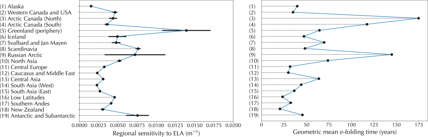
Fig. 4. Left: relative regional volume sensitivity to ELA perturbations ( $\Sigma _r$) and the uncertainty estimates (black lines). Right: mean response time as a geometric mean e-folding time for each region.
Using the regional ELA distance ( $d_r$; Eqn (19)), we find that Antarctic and Subantarctic, Svalbard and Scandinavia (267, 322 and 326 m, respectively) are the most threatened by the complete disappearance of glaciers, while Alaska, South Asia West and Caucasus and Middle East are the least (1645, 1250 and 1074 m, respectively).
Since the regional response time distributions appear to be approximately log-normal, we use the geometric instead of the arithmetic mean to summarize them. The mean global response time of glaciers is 49 years, with the slowest response time estimated for Arctic Canada (North and South) and Russian Arctic (175, 117 and 145 years, respectively; Fig. 4), while the fastest is calculated for New Zealand, Low Latitudes and Caucasus and Middle East (17, 21 and 28 years, respectively).
We find that the response (e-folding) time estimates are consistent with those of previous studies. Haeberli and Hoelzle (Reference Haeberli and Hoelzle1995) estimated typical response times of glaciers larger than 0.2 km2 in the European Alps as 20--40 years, commensurate with our mean of 27 years for Central Europe. Using the Jóhannesson and others (Reference Jóhannesson, Raymond and Waddington1989) expression for response time, Cuffey and Paterson (Reference Cuffey and Paterson2010) estimated response times between 150 and 600 years for high polar glaciers with thicknesses between 150 and 300 m. The mean response time in our model for glaciers in this thickness range in polar regions is 179 years. In general, Eqn (11) predicts longer response times than the volume response time of Jóhannesson and others (Reference Jóhannesson, Raymond and Waddington1989); this is because our model includes the feedback between glacier thickness change and mass balance (Cuffey and Paterson, Reference Cuffey and Paterson2010).
Our model is ‘perfectly plastic’ (Harrison and others, Reference Harrison, Raymond, Echelmeyer and Krimmel2003) or ‘one-stage’ (Roe and Baker, Reference Roe and Baker2014), i.e., the glacier area responds instantly to volume changes. The model, therefore, does not consider the time it takes for mass to get redistributed by ice flow and for the terminus slope to steepen in advance, or to flatten in retreat (Roe, Reference Roe2011). Consequently, when forced into an advance a real glacier will remain shorter than what is predicted by our model, experiencing less melt and gaining mass faster, while the opposite is true in retreat, leading to a faster response time for volume in reality than predicted by our model. For glacier length, on the other hand, the omission of these processes in our model results in shorter response times than in flowline models and leads to different spectral properties of glacier as filters for high-frequency climate forcing (Roe, Reference Roe2011; Roe and Baker, Reference Roe and Baker2014). Previous numerical findings have shown that a similar one-stage model responds more quickly to perturbations in mass balance than flowline or multiple-stage models (Roe, Reference Roe2011; Roe and Baker, Reference Roe and Baker2014). However, in the same studies, the final equilibrium values simulated across the models closely agree, as well as the spectral properties for low-frequency climate forcing. Our model can, therefore, be used for approximating glacier response close to an equilibrium, but it may be unsuitable for projecting glacier evolution in response to future climate scenarios from global climate models.
The fact that our model has a uniform hypsometry (a constant width along the glacier length) affects the accuracy of the estimated response and equilibrium glacier volume. For example, glaciers with a wide upper basin and narrow tongue are expected to have larger equilibrium lengths than those with a more uniform hypsometry (Oerlemans, Reference Oerlemans2008). Although most glaciers have hypsometry data in the RGI, it remains a challenge to incorporate a glacier geometry of high complexity into a low-dimensional dynamical model.
Considering that the variability in modeled glacier sensitivities and response times is driven by an overall effect of multiple geometric and climatic factors, we next investigate whether some of this variability can be attributed to individual factors, in particular, glacier size (volume) and slope. To get a general idea, we plot the modeled sensitivities and response times of all glaciers in the dataset against the two model variables (Fig. 5). There is a negative correlation between normalized sensitivity (sensitivity divided by steady-state volume) and volume, indicating that larger glaciers generally lose a lesser percentage of their volume when the temperature is increased (Fig. 5, top right). For comparison, normalized sensitivity appears to have neither a positive nor a negative linear relationship with glacier surface slope (Fig. 5, top left). Previous work has suggested that steeper slopes lead to shorter response times (Haeberli and Hoelzle, Reference Haeberli and Hoelzle1995), which is consistent with our results (Fig. 5, bottom left). Although in Harrison's original model larger glaciers have slower response times, volume scaling predicts that larger valley glaciers have a shorter response time, all other variables being held constant (Bahr and others, Reference Bahr, Pfeffer, Sassolas and Meier1998). This relationship between response time and volume has also been verified using finite element simulations of ice flow (Pfeffer and others, Reference Pfeffer, Sassolas, Bahr and Meier1998). When other factors are taken into account (e.g., altitude range) there is often a more complex relationship between response time and size, if at all (Raper and Braithwaite, Reference Raper and Braithwaite2009). Indeed, our results do not reveal a clear global relationship between response time and volume (Fig. 5, bottom right). As in Raper and Braithwaite (Reference Raper and Braithwaite2009), we find that the dependence of response time on size varies by region: in some regions we find response time to have a moderate negative correlation with volume.
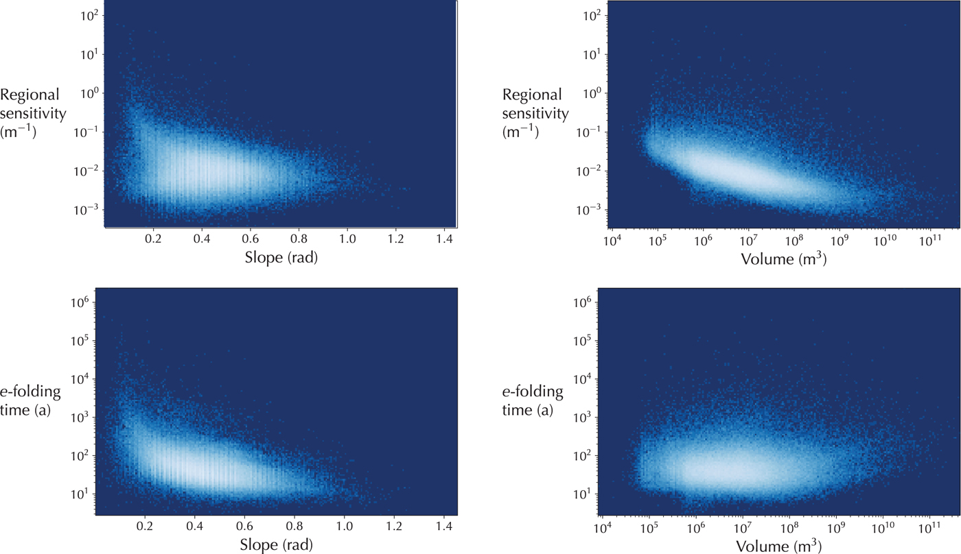
Fig. 5. Normalized sensitivity (sensitivity divided by steady-state volume) versus volume and slope (top panels) for all glaciers in the dataset. Response time versus volume and slope (bottom panels). Lighter colors in the plot correspond to a greater number of clustered points.
Using uncertainty propagation with the input uncertainties as described in Appendix B, the median absolute uncertainty in the response time is 27 years. The median percentage uncertainty is 45% in the sensitivity to ELA and 61% in the response time.
4.2. Effect of geometric and climatic factors
To interpret the sensitivity and response time results, we ran HSIC sensitivity analyses on the (unnormalized) volume sensitivity and response time data. Again, we exclude glaciers with an equilibrium volume of zero, since the sensitivity and response time cannot be meaningfully defined for these cases. The results as  $S_i$ indices for each variable are shown in Figure 6, where a larger $S_i$ indicates a larger dependence of the volume sensitivity (or response time) on the given variable. For the volume sensitivity the dominant drivers appear to be glacier volume and the constant of proportionality in the volume-length scaling, while for the response time the dominant drivers are the mass-balance gradient in the ablation area and the surface slope.

Fig. 6. HSIC indices for the sensitivity and response time. The bars indicate the 95% bootstrap confidence intervals.
However, since the sensitivity indices are calculated for each variable individually, they do not take into account the dependencies between variables. Table 3 quantifies the pairwise dependencies between the variables, calculated using the same  $S_i$ indices as for the sensitivities. Because both $c_l$ and $c_a$ are highly correlated with V (Table 3), the final outcome of the analysis is that the primary driver of interglacier differences in volume sensitivity to ELA perturbations is glacier size, followed by the surface slope. Since there are no significant dependencies between the ablation gradient and surface slope, these variables appear as the dominant drivers of differences in glacier response time. The effect of ablation gradient on glacier response time can be understood from the fact that response time is known to depend on the ablation at the terminus (Eqn (12)). In our model, a larger ablation gradient generally corresponds to a shorter response time, which is consistent with theory since a larger ablation gradient causes more terminus ablation. The fact that the ablation gradient is identified as a significant contributor confirms that the climate setting does play an important role in determining glacier response to climate change.
Table 3. Pairwise normalized HSIC (Eqn (21)) for the model data, showing dependence between input variables

In addition to the effect of the geometric and climatic factors on individual glacier response on a global scale, we try to determine whether the regional sensitivities and response times can be related to mean regional quantities. The relationships between the mean regional quantities and the regional sensitivities and response times will not necessarily coincide with the factors found to be significant using the HSIC analysis above, since (1) factors that contribute to the differentiation between regions may not be significant on a global scale and (2) the effect of a certain quantity on individual glacier response may not be evident when its entire distribution is distilled to regional means. We computed the Pearson correlation between the regional sensitivities  $\Sigma _r$ and regional mean response times on the one hand, and the regional means of V, $c_l$, $c_a$, $G^{\ast}$, $\dot {g}_{\rm abl}$, β and the regional ELA distances $d_r$ on the other.
The regional means of response times were most strongly correlated to the regional mean  $c_a$, $c_l$ and $\dot {g}_{\rm abl}$ (r = 0.88, 0.86 and $-0.87$ respectively, all with p-values < $3\times 10^{-6}$), in addition to V (r = 0.76, p-value $1.5\times 10^{-4}$) and β (r = −0.79, p-value $6.0\times 10^{-5}$). Interestingly, mean regional volume was positively correlated with mean regional response time, despite the fact that on a global level there is not a clear relationship between volume and response time (Figs 5, 6), and within some regions there is a negative correlation. This may be a result of the negative correlation within regions masking the positive correlation between regions, such that globally there is no net correlation visible. The regional sensitivities only showed a significant correlation to the regional ELA distances $d_r$ (r = −0.71, p-value $7.4\times 10^{-4}$). This is because sensitivity to ELA is an indirect measure of closeness to the bifurcation: the sensitivity to ELA (Eqn (16)) is proportional to $\partial V_s^{\ast}/\partial P^{\ast}$, and that quantity diverges to negative infinity as the bifurcation is approached (note, however, that away from the bifurcation $\vert \partial V_s^{\ast}/\partial P^{\ast} \vert$ also increases).
5. CONCLUSIONS
By building on a block model proposed by Harrison (Reference Harrison2013), we showed that a low-complexity dynamical model together with glacier inventory data can be successfully used to characterize features of glacier response to climate change. In particular, we used it to estimate regionally differentiated response times and sensitivities to ELA changes. We applied global sensitivity analysis, based on the Hilbert–Schmidt Independence Criterion, to quantify the contribution of different model input variables to the model output over the entirety of the input distribution. The results show that volume sensitivity is mainly driven by the glacier size distribution, followed by the surface slope. On the other hand, the glacier response time estimates are mainly driven by the climatic setting as captured in the ablation gradient, followed by glacier surface slope. Global sensitivity analysis presents a powerful tool in modeling physical systems, not only for interpretation of outputs as demonstrated here, but also for model reduction and identification of variables that cause the most uncertainty in the output (Saltelli and others, Reference Saltelli2008). Possible future work is to convert the simple block model into a multiple-stage model, which could be used in concert with global climate models to make projections of glacier volume, and to validate the simulations with historic glacier data.
Acknowledgments
Funding supporting this study was provided through the Natural Sciences and Engineering Research Council (NSERC) of Canada (Discovery Grants to V. Radić and C. Schoof). We thank M. Huss for providing the global estimates of glacier thickness.
APPENDIX A. ROOT-FINDING METHOD
We consider the non-negative roots of functions of the type
 $$ f\,(x) = c_0 x^{n_0/d_0} + c_1 x^{n_1/d_1} + \cdots + c_m x^{n_m/d_m},$$
with x and the coefficients  $\{c_i\}$ real, and the exponents $\{n_i/d_i\}$ nonnegative rationals expressed in lowest terms. These types of functions are sometimes called fractional polynomials (since they resemble polynomials, but have rational exponents). To find the roots, we make a substitution that transforms $f(x)$ to a polynomial function. Let $l = {\rm lcm} \{ d_i\} $ and $g=\gcd \{n_i\}$. Then, $f(y^{l/g})$ is a polynomial in y, since all the $\{d_i\}$ are factors of l and all the $\{n_i\}$ are multiples of g. The roots of this polynomial, $\{y^{\ast}_i\}$, can be found numerically using eigenvalue methods (Edelman and Murakami, Reference Edelman and Murakami1995). The roots of $f(x)$ in x will then be $\{{y^{\ast}_i}^{l/g}\}$.
APPENDIX B. UNCERTAINTY IN THE INPUT QUANTITIES
For glaciers with available thickness estimates, we assume a thickness uncertainty of 30%, the estimated error in Huss and Farinotti (Reference Huss and Farinotti2012). For glaciers whose thicknesses are calculated as a function of the surface area, we use an uncertainty given by the root-mean-square relative error in the regression on a test sample, i.e., a sample independent of the data used for model calibration and validation. We assume a length uncertainty of 20% following the estimates by Machguth and Huss (Reference Machguth and Huss2014) for small glaciers (the percent uncertainty in larger glaciers is smaller). We use the root-mean-square cross-validation error on a test set for the uncertainty in the mass-balance gradients (0.32 for  $G^{\ast}$ and 0.0028 a−1 for $\dot {g}_{\rm abl}$). We apply the area uncertainty function suggested by Pfeffer and others (Reference Pfeffer2014) to assess the glacier area error.
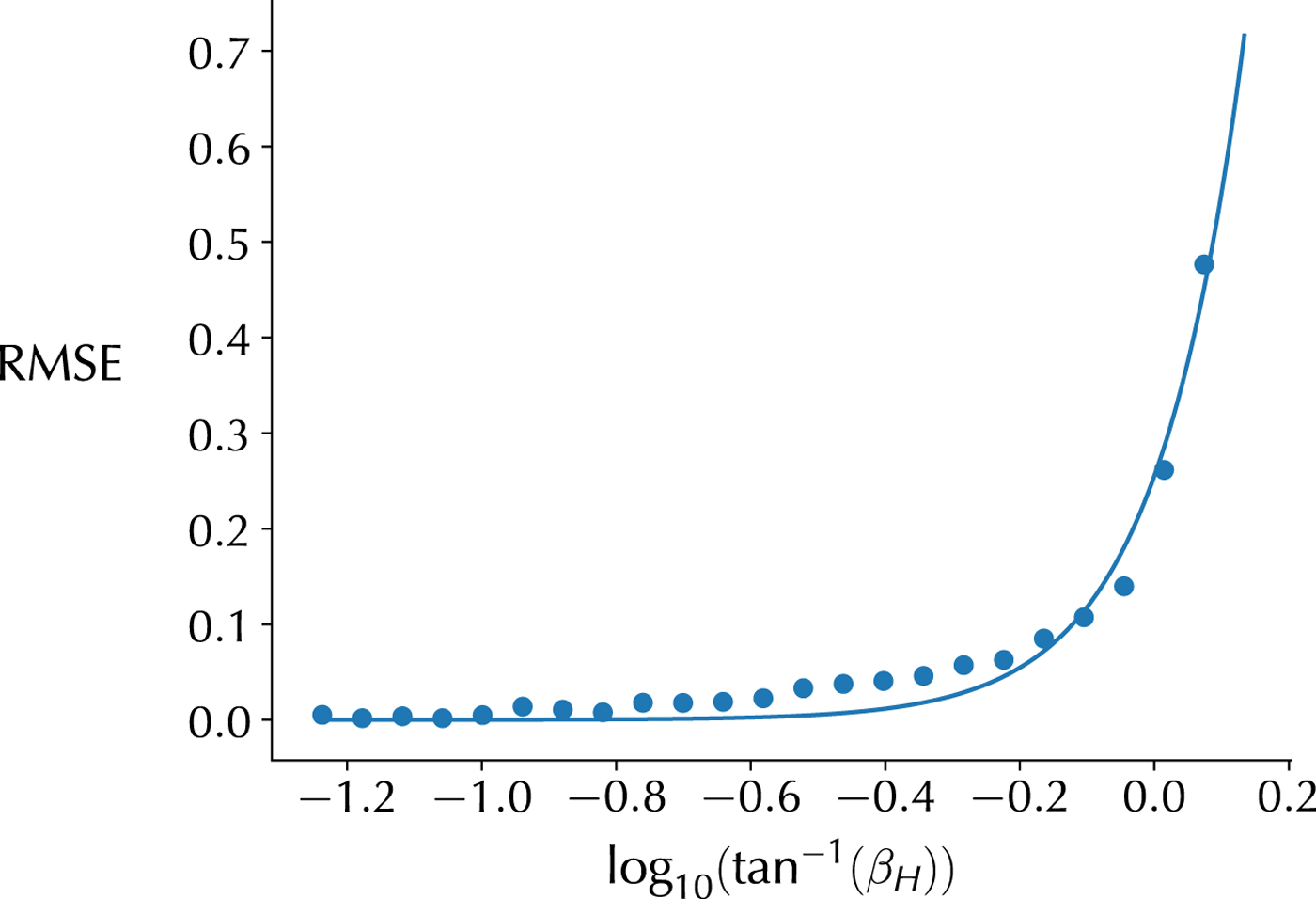
Fig. B1. RMSE as a function of  $\beta _H$. The points are the computed errors, and the line is the interpolated function.
To estimate the uncertainty for surface slope β, we compare the average slopes in the RGI to those given in Huss and Farinotti (Reference Huss and Farinotti2012). Instead of the arithmetic mean used in the calculation of the mean slope in the RGI (calculated using the discretized topography along the glacier's centerline), Huss and Farinotti (Reference Huss and Farinotti2012) use a weighted mean, giving smaller weights to very steep slopes in an elevation band. To estimate the error function we partition the set of slopes into evenly spaced bins in log space (in order to more accurately account for small slopes, to which the model is more sensitive) and then compute the RMSE in each bin. We fit a power function of the form  ${\rm RMSE}(\beta _H) \!=\! \sqrt {E [{({\tan }^{ - 1}\beta _H - {\tan }^{ - 1}\beta _R)}^2]} \!=\! c(\tan ^{ - 1}\beta _H)^r$, where $\beta _H$ is the slope from Huss and Farinotti (Reference Huss and Farinotti2012) and $\beta _R$ is the slope from the RGI. We find $c \simeq 0.255$ and $r \simeq 3.349$ to give the best fit (Fig. B1).


 Open access