


Introduction
Carbon dioxide is the most important greenhouse gas directly impacted by human activities. The atmospheric CO2 mixing ratio has increased 25% since the industrial revolution (Reference Etheridge, Steele, Langenfelds, Francey, Barnola and MorganEtheridge and others, 1996; Reference MacFarling MeureMacFarling Meure and others, 2006), and its continuing increase will contribute a major fraction of future global warming (Reference SolomonSolomon and others, 2007). The transfer of carbon between reservoirs in the carbon cycle ultimately controls the fate of fossil-fuel-derived CO2, but how climate and the carbon cycle are linked is only partly understood. Studies of how atmospheric CO2 and climate are related in geologic history contribute to our understanding of Earth’s climate system. Ice cores are unique archives that allow direct measurement of atmospheric CO2 content over 800 ka (Reference MacFarling MeureMacfarling Meure and others, 2006; Reference LüthiLüthi and others, 2008), expanding instrumental CO2 records, which began only in 1958 (C.D. Keeling and T.P. Whorf, http://gcmd.nasa.gov/records/GCMD_CDIAC_CO2_SIO.html). CO2 records derived from Antarctic ice cores are widely demonstrated to be representative of atmospheric concentrations over several glacial–interglacial cycles (Reference Fischer, Wahlen, Smith, Mastroianni and DeckFischer and others, 1999; Reference PetitPetit and others, 1999; Reference Kawamura, Nakazawa, Aoki, Sugawara, Fujii and WatanabeKawamura and others, 2003; Reference Siegenthaler, Stocker, Monnin, Lüthi, Schwander and StaufferSiegenthaler and others, 2005; Reference LüthiLüthi and others, 2008). However, this is not the case for CO2 records from Greenland ice cores where dust is present in high concentration. The dust includes carbonates (Reference Anklin, Barnola, Schwander, Stauffer and RaynaudAnklin and others, 1995, Reference Anklin1997; Reference Barnola, Anklin, Porcheron, Raynaud, Schwander and StaufferBarnola and others, 1995; Reference Smith, Wahlen, Mastroianni and TaylorSmith and others, 1997a,Reference Smith, Wahlen, Mastroianni, Taylor and Mayewskib) and organic compounds (Reference Tschumi and StaufferTschumi and Stauffer, 2000) within the ice core, giving rise to in situ CO2 production. There is general agreement of atmospheric CO2 trends within deep Antarctic ice cores on millennial and longer timescales. However, disagreements in CO2 concentrations of up to ∼5–20 ppm between comparable cores and laboratories have been reported (Reference Fischer, Wahlen, Smith, Mastroianni and DeckFischer and others, 1999; Reference PetitPetit and others, 1999; Reference Stauffer and EliasStauffer, 2006).
Given these discrepancies, there is an increasing demand for high-precision measurements combined with high-temporal-resolution CO2 concentration records, to decipher the exact mechanisms controlling Earth’s climate system on millennial or sub-millennial timescales. For example, understanding how atmospheric CO2 varied with respect to abrupt climate change during the last ice age (e.g. Reference StaufferStauffer and others, 1998; Reference Ahn and BrookAhn and Brook, 2007, Reference Ahn and Brook2008) or during climate cycles of the late Holocene (Reference MacFarling MeureMacFarling Meure and others, 2006) requires, in some cases, decadal data with a precision of at least 2 ppm, and preferably better. In addition, in deep ice-coring projects ice availability is limited, requiring analytical techniques suitable for small samples of <10 g. We note that the air age distribution also limits time resolution. Usually, low accumulations at coring sites give large age distributions and limit time resolution of gas records in ice cores (Reference Spahni, Schwander, Flückiger, Stauffer, Chappellaz and RaynaudSpahni and others, 2003).
Analysis of CO2 in a small quantity of ice is challenging, primarily because of variable desorption and adsorption of CO2 in the extraction line and chamber due to water-vapor content (Reference Zumbrunn, Neftel and OeschgerZumbrunn and others, 1982). Air should be extracted using a ‘dry’ mechanical method rather than simpler ‘wet’ extraction (melting under vacuum), as melting may induce a carbonate–acid reaction and increase CO2 levels in the sample (Reference Delmas, Ascencio and LegrandDelmas and others, 1980). Conventional dry extraction methods include crushing ice with metal needles (Reference Zumbrunn, Neftel and OeschgerZumbrunn and others, 1982; Reference Wahlen, Allen, Deck and HerchenroderWahlen and others, 1991) or metal balls (Reference Delmas, Ascencio and LegrandDelmas and others, 1980), milling with blades (Reference Moor and StaufferMoor and Stauffer, 1984; Reference NakazawaNakazawa and others, 1993) or a ‘cheese grater’ (Reference Etheridge, Pearman and de SilvaEtheridge and others, 1988). All methods require sustained cold conditions in the vacuum chamber. We chose to build a ‘needle crusher’ (Fig. 1) capable of crushing small (∼10 g) ice samples. The milling techniques and crushing with metal balls at present require relatively large samples (>500 and ∼40–50 g for blades and metal balls, respectively).
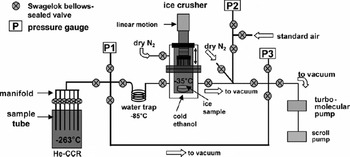
Fig. 1. Schematic diagram of the newly developed dry extraction system at Oregon State University for paleoatmospheric CO2 trapped in ice cores. See text for details. He-CCR indicates a helium closed-cycle refrigerator.
The infrared laser spectroscopy (IRLS) method has been used successfully in several laboratories for analysis of air (<1 cm3 STP) extracted from small ice samples (<10 g; Reference Zumbrunn, Neftel and OeschgerZumbrunn and others, 1982; Reference Wahlen, Allen, Deck and HerchenroderWahlen and others, 1991). However, the analytical precision with IRLS is generally ∼0.5% (1σ), corresponding to 1.5 ppm CO2 for measurements of bubble-free single-crystal ice (Reference MonninMonnin and others, 2001; Reference LüthiLüthi and others, 2008). Instead, we used gas chromatography (GC) to analyze the small amount of air liberated from ∼8–15 g ice. Utilizing this technique under optimized conditions, we obtained good precision, ∼0.3–0.4% for the Siple and Taylor Dome bubbly ice (pooled standard deviations), corresponding to ∼0.9 ppm in glacial or interglacial ice. An additional advantage of this technique is the potential to simultaneously measure other gas species in addition to CO2 (e.g. CH4 and N2O (not described in this paper)). Here we describe our method, its application to several ice cores and the potential of our system for use in future ice-core studies.
Dry Gas Extraction
Our extraction system is composed of three main components: a vacuum system, a crushing system and a cryogenic cold trap to condense air released from the crushed ice (Fig. 1).
The pumping system is composed of a turbomolecular pump backed by a dry (scroll) pump, ensuring a clean vacuum system. Electropolished stainless steel was used for all vacuum lines. Parts are connected by VCR fittings with clean Swagelok® OFHC copper gaskets. Bellows-sealed Swagelok® valves with stainless-steel stem tips are used. Pressure gauges exposed to samples (P1 in Fig. 1) and standards (P2) are ultra-clean MKS products (Baratron® capacitance manometer 626 for P1 and Baratron® pressure transducer 750 for P2). The crushing chamber is a custom-designed double-walled stainless-steel vacuum chamber sealed with ConflatTM flanges. Using a closed-circulation chiller (Lauda Proline RP855), cold ethanol is circulated between the inner and outer walls to cool the chamber to temperatures that can be controlled to as low as −35 to −40°C. The inner volume of the crushing chamber is ∼200 cm3. Ice is crushed with a ‘needle plate’, a stainless-steel plate containing 91 steel pins, affixed to a heavy-duty pneumatically actuated bellows-based linear motion feedthrough (MDC Vacuum Products). The size of crushed ice particles is mostly <1 mm. The extraction efficiency for crushing samples of 8–13 g is generally ∼80–90% (efficiency is the amount of air extracted divided by total air in the sample) for bubbly ice. With larger samples the efficiency decreases. Slight redesign of the pin end shape or pin number density may improve extraction.
The exchange gas cryostat accommodates six stainless-steel sample tubes (Fig. 1), sealed with Swagelock™ bellows-sealed valves, and can cool the tubes to 10.5 K. The cryostat was constructed to our specifications by Janis Research Corporation, and allows the tubes to be replaced after a set of gas extractions, allowing faster analysis. Each stainless-steel sample tube is ∼39.3 cm long with 0.63 cm outer diameter and an internal volume of ∼6 cm3. One end was closed by welding. A manifold system connects gas extracted from the ice to six sample tubes.
Analytical procedures are as follows. The crushing chamber, sample tubes and extraction line are pumped under vacuum overnight. On the morning of extraction, ice samples are carefully trimmed to remove ∼0.5–2.0 cm of surface ice, and then cut into a ∼3–4 cm diameter disk with thickness ∼1.0–1.5 cm. Sample size varies from 8 to 15 g. Ice samples are stored and cut in a walk-in freezer at −25°C. Ice samples are loaded into the ice crusher by opening the crusher while ultra-pure N2 gas is flushed to the top and bottom sections (Fig. 1). After loading, the crusher is sealed with a Cu gasket. After pumping the chamber for ∼10–15 min the ice is crushed, typically taking ∼10–30 s for the bubbly ice. Some ice samples have no bubbles but air is trapped in the ice crystal lattice (clathrate) at great depths and this ice is harder to crush than bubbly ice. We crush for ∼60–180 s for the clathrate ice, with a frequency of about one or two strokes per second. The liberated air is expanded to a stainless-steel coil water trap in an ethanol Dewar flask at approximately −85°C to dry the air for 3 s. The air is then expanded to pressure gauge P1 (Fig. 1) to measure the amount of gas liberated. Finally, the air is expanded to the manifold and condensed in a 0.63 cm stainless-steel sample tube housed in a cryogenic system at ∼10.5 K. Gas condensation is monitored by pressure gauge P1. Typically, the pressure in the crusher drops below the detection limit (10 mtorr) in <90 s. To ensure complete trapping of air in the sample tube, we open the tube valve for 180 s for bubbly ice. For deep clathrate ice from the Byrd ice core, an additional 90 s for degassing prior to gas trapping was allowed, and an additional 60 s of trapping (total of 330 s after crushing the ice) was deemed necessary. This was because clathrate ice from the Byrd ice core showed slow degassing after crushing.
The CO2 content of the analyzed air is affected by adsorption and desorption of CO2 in the crusher, extraction line and sample tubes. The net effect is measured by introducing standard air over the ice sample in the crusher and following the same gas-extraction procedure as for a crushed sample. This is referred to as an ‘internal standard’. Each measurement for a crushed sample is corrected by adding the offset of the internal standard to, or subtracting it from, its calibrated value for that standard. CO2 measurements for internal introduced standards prepared before and after crushing ice usually differed by ∼1 ppm, occasionally up to 2 ppm. To make a precise correction for the measurements for Taylor Dome M3C1 and Siple Dome cores, we based the correction on the mean of internal standards introduced before and after crushing each ice sample. In a given day, we routinely measured two to four ice samples in the early stage of method development, then increased the number of samples to four to six by adding a multiple manifold-tube system.
The crushing process itself might also alter the CO2 content of an extracted sample, perhaps due to CO2 production or degassing from flexing of the metal bellows. To examine the importance of this issue we crushed air-free ice in the presence of standard air. We made air-free ice by boiling deionized water in a cylindrical vacuum chamber with a ∼30 cm long, 0.32 cm diameter tube fixed to the outlet of a high-vacuum valve fixed to a Conflat™ flange that seals the chamber. Boiling for 30 min drives both steam and air from the vessel, and the vacuum valve is closed at the end of the boiling process to prevent laboratory air from entering the chamber. The water in the chamber is frozen slowly in an ethanol bath to create air-free ice. We found that crushing caused 0.96 ± 1.02 (1σ) ppm CO2 enrichment of standard air (n = 11 measurements on six different days over 3.5 months).
Gas Chromatography
We applied GC to the small quantity of air extracted (∼1 cm3 at STP) from ∼8–15 g of ice. Before analysis by GC, sample tubes containing the trapped air were warmed for 10 min in a water bath set to ∼50–60°C. The line used for the GC system was pumped using a turbomolecular pump backed with a scroll pump, in the same way as the gas extraction line.
All measurements in this study were performed using an Agilent 6890N GC. The GC system is fitted with a Ni catalyst that converts CO2 to methane, which is subsequently detected by a flame-ionization detector. The GC settings and other parameters are shown in Table 1. N2 rather than He is used as the carrier gas, because the detector is more stable over a greater range of air-flow rate and temperature conditions with the N2. Signals are acquired and integrated using Agilent ChemStation software. Air samples in the tubes are expanded to the GC via a vacuum inlet line connected to a sample loop (5 cm3) installed on a six-port two-position Valco valve. Owing to the small sample size, the loop is kept under vacuum. Sample pressure in the loop is generally 10–40 torr, and is measured with a high-precision MKS 622 Baratron capacitance manometer (accuracy >0.15%). The gas pressure in the sample loop depends on temperature. The sample loop is mounted outside the GC, and temperature variations could produce variability in our results. To test the significance of temperature-dependent variability, we conducted some measurements with the loop mounted in the GC oven, where the temperature was set to 60°C. Data precision was not improved, indicating that temperature variations in the laboratory are not large enough to create a detectable effect.
Table 1. Settings for gas chromatography

The GC system was calibrated with dry standard air of known CO2 concentration from one of two standard air cylinders, 197.54 or 291.15 ppm (±0.01 ppm; US National Oceanic and Atmospheric Administration (NOAA) Earth System Research Laboratory, Global Monitoring Division). The standard air was directly introduced to the sample loop at a pressure range comparable to the sample air aliquots. Typical daily precision for standard air is ∼0.2 ppm (1σ) for n = 5–10 measurements (197.54 or 291.15 ppm).
A daily calibration curve was constructed using a second-order polynomial fit to the CO2 peak area vs total air pressure for the aliquots of standard air. We determined the unknown CO2 mixing ratio of the sample air using the linear relationship between the ratio of peak area to air pressure and the CO2 mixing ratio. Details are as follows.
First we fit a second-order polynomial equation to the CO2 peak area vs air pressure in the sample loop
where A represents a peak area integrated in the GC, P
air is air pressure in the sample loop before measurement and a, b and c are coefficients obtained by regression. To obtain the coefficients of Equation (1), several measurements were performed for standard air over the pressure range expected for air samples extracted from ice. The second-order coefficient is four orders of magnitude lower than the first-order coefficient, but using the second-order equation slightly improves precision (0.1 ppm CO2 or less) relative to a linear relation. Coefficient c in Equation (1) represents the blank in GC analysis. A test with ultra-zero air (<0.5 ppm CO2) gave a peak area that falls within the range of values determined for c in daily calibration curves over a 2 year period. Thus, the effective signal ![]() is proportional to P
air and the CO2 mixing ratio, [CO2], and the unknown CO2 mixing ratios of the air samples are determined by
is proportional to P
air and the CO2 mixing ratio, [CO2], and the unknown CO2 mixing ratios of the air samples are determined by
In order to test the linearity between [CO2] and ![]() , we developed a calibration curve with standard air of low CO2 concentration (197.54 ppm) and then analyzed a different standard air with a CO2 mixing ratio of 291.15 ppm. The difference between estimation by measurements and assigned concentration was 0.2–1 ppm on average over the course of 2 years. Determination of a low-CO2 content (197.54 ppm) standard air with a calibration using a high-CO2 content (291.15 ppm) standard air gave similar differences between the assigned and measured values. These two standards span most of the range expected for late Quaternary CO2 concentrations (Reference Siegenthaler, Stocker, Monnin, Lüthi, Schwander and StaufferSiegenthaler and others, 2005). Gas-chromatographic techniques can yield non-linear responses and, in principle, two air standards might not completely describe the detector response. However, we measured the standard air over a wide range of absolute quantities of CO2 (wide range of pressures in the sample loop), and obtained a good linearity between the two tanks. These observations support the conclusion that the GC response is linear between the two concentrations. To account for daily drift in the analysis, the run sequence alternates between sample and standard, so that every two to six samples (total 6–12 runs, 2 runs for each air sample) were bracketed by three or four standard air analyses.
, we developed a calibration curve with standard air of low CO2 concentration (197.54 ppm) and then analyzed a different standard air with a CO2 mixing ratio of 291.15 ppm. The difference between estimation by measurements and assigned concentration was 0.2–1 ppm on average over the course of 2 years. Determination of a low-CO2 content (197.54 ppm) standard air with a calibration using a high-CO2 content (291.15 ppm) standard air gave similar differences between the assigned and measured values. These two standards span most of the range expected for late Quaternary CO2 concentrations (Reference Siegenthaler, Stocker, Monnin, Lüthi, Schwander and StaufferSiegenthaler and others, 2005). Gas-chromatographic techniques can yield non-linear responses and, in principle, two air standards might not completely describe the detector response. However, we measured the standard air over a wide range of absolute quantities of CO2 (wide range of pressures in the sample loop), and obtained a good linearity between the two tanks. These observations support the conclusion that the GC response is linear between the two concentrations. To account for daily drift in the analysis, the run sequence alternates between sample and standard, so that every two to six samples (total 6–12 runs, 2 runs for each air sample) were bracketed by three or four standard air analyses.
Results
To demonstrate system performance we analyzed samples from several Antarctic ice cores from various glaciological environments (Table 2). Precision of replicate measurements can vary from core to core and depth to depth due to ice quality (fractures, recrystallization, etc.) or chemical impurities. The formation of clathrates at depth also influences the reproducibility of CO2 measurements by dry extraction. This will be discussed below.
Table 2. Characteristics of Antarctic ice cores from which CO2 was measured

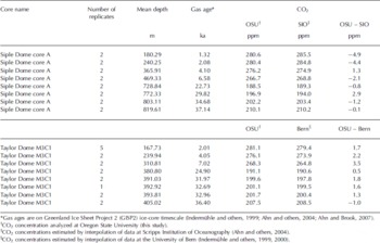
Duplicate measurements of 8–11 g samples from the Siple Dome A core (Fig. 2a) and Taylor Dome M3C1 core (Fig. 2b) were made and the pooled standard deviations for these duplicates are 0.84 (16 samples from 8 depths) and 0.83 ppm (18 samples from 8 depths), respectively (Table 3). This is comparable to the best results from the average of four to six replicates at other facilities. Siple Dome ice for the last glacial age was highly fractured and we avoided the fractures by trimming. The good agreement between duplicate samples from the Siple Dome core indicates that the contamination due to invisible fractures and/or drill fluid is negligible. In Figure 2 the results are compared with previous measurements at the Scripps Institution of Oceanography (SIO; Reference AhnAhn and others, 2004) for Siple Dome, and the University of Bern (UB; Reference IndermühleIndermühle and others, 1999, Reference Indermühle, Monnin, Stauffer, Stocker and Wahlen2000) for Taylor Dome. The individual measurements for Oregon State University (OSU) are plotted, whereas data presented from UB and SIO are the mean of four to six measurements for each depth. Our data agree with those from SIO and UB for the nearest sample depths, within 5 ppm (Table 4). The glacial samples agree better than those of the Holocene, within 2 ppm except at one depth. As we have not measured exactly the same samples it is difficult to know whether differences are due to real variability in atmospheric CO2, differences in standard scales or other analytical offsets. We are participating in an international laboratory intercomparison exercise for ice-core gases, including CO2, which should clarify some of these issues.

Fig. 2. (a) Comparison of Siple Dome CO2 data measured at OSU with data from the SIO (Reference AhnAhn and others, 2004). (b) Comparison of Taylor Dome CO2 data measured at OSU with data from the University of Bern (Reference IndermühleIndermuhle and others, 1999, Reference Indermühle, Monnin, Stauffer, Stocker and Wahlen2000). In most cases the replicates were measured several months apart and agree to better than 1 ppm (see Table 4).
Table 3. CO2 concentrations from Antarctic ice cores from this study
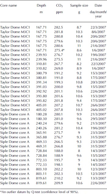
Table 4. Comparison of CO2 concentration results among different laboratories
We also measured CO2 in several samples from a shallow ice core (<300 m) drilled at the WAIS (West Antarctic ice sheet) Divide site. WAIS Divide is the site of a new deep-drilling program conducted by the US National Science Foundation, with a major objective of obtaining high-resolution greenhouse-gas records. We measured seven samples, two of which included a bubble-free layer ∼1 mm thick, which is common in shallow cores from the WAIS Divide site. It is not known whether the layers are refrozen melt layers or snow crusts. However, these layers were initially a concern because of reports that melt layers can artificially enrich the CO2 content of the ice (Reference Neftel, Oeschger, Schwander and StaufferNeftel and others, 1983; Reference Stauffer, Neftel, Oeschger, Schwander, Langway, Oeschger and DansgaardStauffer and others, 1985; Reference Ahn and BrookAhn and others, 2008). We did not detect any enrichment associated with the bubble-free layer, and replicate analysis of ice in a 9 cm section at a depth of 297.6 m and a 3 cm section at 140.9 m gave 1σ precisions of 1.2 and 1.5 ppm, respectively. This confirms that the bubble-free layer does not significantly affect the CO2 content. In addition, the excellent results from this ice show that records from WAIS Divide will allow measurements of small variations, of 10 ppm or less, for the last 1000 years (Reference MacFarling MeureMacFarling Meure and others, 2006). The precision will be enhanced by replicate measurements. This is encouraging for future studies of the deep WAIS Divide ice cores.
CO2 data from the Byrd ice core were obtained as part of a project to understand the role of CO2 in millennial-scale climate variability during the last ice age (Reference Ahn and BrookAhn and Brook, 2007, Reference Ahn and Brook2008). CO2 variations among replicate ice samples from the Byrd ice core at matching depths gave a pooled standard deviation of ∼3.0 ppm for 14 samples from 7 depths. This is much larger than those of the Siple Dome and Taylor Dome ice cores (<1 ppm). We expedited the experimental process and employed an average of two or three internal standards for two to four ice samples (Reference Ahn and BrookAhn and Brook, 2007, Reference Ahn and Brook2008). As such, not every sample was paired with a standard introduced before and after crushing, as described above. Using this method, the pooled standard deviation for 382 samples from 171 depths was 3.4 ppm after rejecting data from 4 depths (Reference Ahn and BrookAhn and Brook, 2007, Reference Ahn and Brook2008). We reduced the data uncertainty by making replicate measurements. The standard deviation of the mean for samples with two to five replicates averaged 1.5 ppm. Using these new data from ∼90–20 ka, a new chronology for CO2 was established. This was synchronized with Greenland ice-core records to study the link between high-latitude climate change and the carbon cycle during the last glacial period (for further discussion see Reference Ahn and BrookAhn and Brook, 2007, Reference Ahn and Brook2008).
Discussion and Future Directions
Our methods show excellent extraction and analytical performance for bubbly ice from Siple Dome, Taylor Dome and shallow WAIS Divide coring sites. Clathrate Byrd ice shows larger scattering of the data, although the uncertainty is still good enough to address current scientific issues. It is not clear whether this uncertainty is due to the physical properties of the ice or due to alteration during coring (Reference Bender, Sowers and LipenkovBender and others, 1995) or long-term storage (since 1968). Stauffer and others (2000) observed slow degassing after crushing of clathrate ice samples. Owing to different degassing kinetics for specific gas species, the CO2 mixing ratio changes with time (Stauffer and others, 2000) in the crusher and may give a low CO2 mixing ratio for the short degassing period from the clathrate ice. Our method allowed more than 5.5 min for degassing. A longer degassing time would increase the desorption and adsorption of CO2 in the extraction system and the precision would deteriorate. With the deepest ice core, at a depth of over ∼2000 m, we observed an ∼8–10% increase in gas pressure in the crusher 35–95 s after crushing. After 240 s of trapping sample air in the sample tube (total 330 s after ice crushing) from clathrate ice originating from Byrd ice, we usually observed a pressure of ∼10 mtorr or less in the extraction line (P1; Fig. 1), indicating very little degassing from the ice. In order to check if our degassing time was sufficient, we also allowed 90–120 s longer trapping time (total 420–450 s after crushing) for several pairs of ice samples, but we observed no significant change in the mixing ratio, implying that our extraction time was sufficient. The appropriate gas extraction time will change from core to core and depth to depth within the same core. This is important, for example, in comparing Holocene CO2 records from bubbly ice with penultimate interglacial CO2 from clathrate ice.
Future studies should also include techniques that allow 100% gas-extraction efficiency without melting the ice. High fractionation of CO2 occurs at depths where air bubbles coexist with clathrate crystals. As such, variable gas-extraction efficiency from bubbles and clathrate crystals gives distorted CO2 mixing ratios (Stauffer and others, 2000; Reference Kawamura, Nakazawa, Aoki, Sugawara, Fujii and WatanabeKawamura and others, 2003). Sublimation techniques allow 100% gas-extraction efficiency; however, the technique requires a long extraction times (Reference Wilson and LongWilson and Long, 1997; Reference Güllük, Slemr and StaufferGüllük and others, 1998) that substantially limit the acquisition of a temporal CO2 series.
Conclusions
We have developed a dry extraction technique for the analysis of CO2 concentration in ancient atmospheric air trapped in ice cores. Our method uses a needle crusher for extraction and GC for analysis of ∼8–15 g of ice. The technique was applied to several Antarctic ice cores, and the overall uncertainty for high-quality samples from Taylor Dome and Siple Dome ice cores was better than 0.9 ppm (1 pooled standard deviation for the total individual ice samples). Our results were also compared with previous results from other laboratories, showing differences of <5 ppm CO2. This technique is suitable for high-precision and high-temporal-resolution studies of ice cores where snow accumulation is high (e.g. the WAIS Divide ice cores), and will improve our understanding of the carbon cycle and, ultimately, Earth’s climate variability.
Acknowledgements
We greatly thank J. Ahrens for assistance in gas-chromatographic analysis and the staff of the US National Ice Core Laboratory for ice sampling and curation. M. Wahlen, K. Kawamura and B. Deck shared their invaluable experimental experience with us. Financial support was provided by the Gary Comer Science and Education Foundation, and US National Science Foundation grant OPP 0337891 to E.J.B.


