


The Gravity Survey
The general location of the ice caps is shown in Figure 1; they are designated as “North”, “West”, “East” and “South” ice cap according to their relative positions. Approximately elliptical in shape, the ice caps lie on the dissected plateau which is the principal topographic form of west Melville Island. The ice caps range in area from 15 to 55 km.2 and lie at an average elevation of 550 m.

Fig. 1. Location of the Melville Island ice caps
The objectives of the gravity survey, performed in June 1963, were to find the general form of the ice bodies and to determine the locations of greatest ice thickness, suitable for a future bore hole for glaciological and heat-flow studies. The survey was performed by the author, a member of the Dominion Observatory Gravity Division affiliated with the Polar Continental Shelf Project (P.C.S.P.).
During a nine-day period 138 gravity stations were established and linked with the gravity control station network established by the Dominion Observatory in the Arctic Islands. Transportation was provided by a Bell 47G-2A helicopter. Gravity measurements were made using a temperature-compensated Worden gravity meter which had a scale constant of 0.40718 mgal/div. Geographical positions of most gravity stations were established by tellurometer traverse and triangulation. Elevations were determined by trigonometric levelling. The stations are separated by intervals of from 0.8 to 2.5 km.
Values of gravity at each station were adjusted for the gravitational effects of varying latitude and elevation according to standard procedures (Reference DobrinDobrin, 1960, p. 187–90) to obtain the Bouguer gravity anomaly. The density of the underlying bedrock, important in carrying out the above reduction, was estimated from the average of 29 dry rock samples: 2.30±0.05 g./cm.3. The Hammer terrain correction chart (Reference HammerHammer, 1939) was used in making corrections for the gravity effect of topographic relief about each station to a radius of 18.8 km. The terrain effect was found to be usually less than 0.5 mgal however in a few cases, it was as high as 2.5 mgal.
Interpretation of the Gravity Data
Accumulations of ice occur at relatively high elevation, usually in mountainous terrain. Because of this the gravity data include significant contributions from effects in addition to the anomaly of a low-density ice body. The gravity effect of irregular topography can be so significant that without adequate topographic mapping in order to calculate the terrain effect, interpretation of the gravity data is severely limited in value. A more subtle difficulty is involved in separating the gravity effect of the ice body from the effect of density variations associated with a possibly complex underlying geology. Detailed geological information is always lacking and because of this, estimates of the “regional” gravity field arising from bedrock density variations, are quite conjectural. These and other difficulties are acknowledged by authors engaged in ice thickness interpretation; Reference LittlewoodLittlewood (1952), Reference Bull and HardyBull and Hardy (1956), Reference ThielThiel and others (1957), Reference RussellRussell and others (1960), Reference Weber and RaaschWeber (1961) and Hyndman (Reference KoernerKoerner and others, 1963, p. 71–72).
The underlying bedrock of this area consists of at least 2,100 m. of flat-lying sandstone of Devonian age, resting on at least 4,500 m. of older sediments of the Franklinian Geosyncline (Reference Thorsteinsson and TozerThorsteinsson and Tozer, 1959). The “regional” anomaly for each ice cap was estimated from the Bouguer anomaly (including terrain correction) at stations established exterior to the ice caps. In all four cases, after the regional anomaly was contoured using this exterior data, it was observed that the gradient is small and almost linear: 0.6, 0.5, 0.4 and 0.6 mgal/km. in a south to south-east direction for the “North”, “East”, “West” and “South” ice caps respectively. A gravity survey of the Melville Island area (Reference SpectorSpector, unpublished) consisting of stations separated at intervals of about 10 km., reveals that the gravity field of a large area including the ice-cap region is indeed slowly varying, confirming the estimate of the regional anomaly made in the ice-cap survey.
In Figure 2, the Bouguer anomaly (including terrain correction) at each gravity station is shown and the data are contoured at 0.5 mgal intervals. Exceptionally low anomalies were observed at two stations on the extreme north-eastern and south-eastern parts of the “North” ice cap and also in the north-eastern part of the “South” ice cap. Contouring of the gravity data in the vicinity of these stations is fairly conjectural because of the lack of neighbouring stations. These anomalies can only be determined by a more detailed gravity survey.
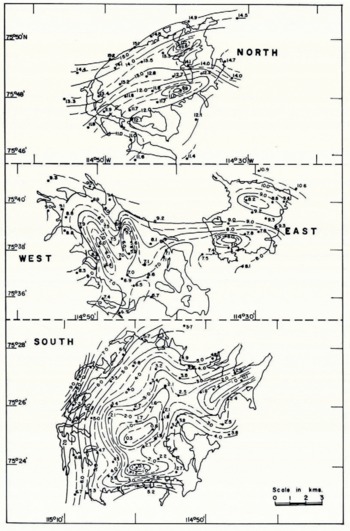
Fig. 2. Bouguer gravity maps of the ice caps, contour interval 0.5 mgal
Figure 3 shows the contoured residual anomaly pattern after the removal of the regional anomaly from the data. Over the major parts of the ice caps, the residual anomaly can be seen to be quite slowly varying. Inherent in this picture is the effect of the wide spacing of the data points achieving a smoothed representation of the actual gravity field.

Fig. 3. Residual gravity maps of the ice caps, contour values in milligals
The uniqueness of gravity interpretations is satisfied in glaciological problems because the upper surface of the “disturbing mass” is known and the problem is reduced to the mapping of a single interface, viz. the ice–bedrock contact. Because of the apparent smoothness of the residual anomaly in the greater portion of each ice cap, the following interpretational technique was chosen, The Bouguer formula,
represents the gravity effect of a slab of ice having a thickness t, a density contrast with respect to underlying bedrock of Δρ and whose horizontal dimensions are very large in comparison to t. The ice density was assumed to be 0.91 g./cm.3, resulting in a density contrast of −1.39 g./cm.3. G is the universal gravitational constant, 6.668×10⁻⁸ in c.g.s. units.
Figure 4. illustrates the interpreted ice distribution. In all four ice caps, the ice body is characterized by two thick zones separated apparently by a bedrock hill. It is surprising that the thickness of ice in these zones is comparatively the same for all four ice caps, namely 30 to 50 m. The ice–rock interface appears to be undulating. The exceptionally low gravity anomalies measured at stations at the north-eastern extremities of both the “North” and “South” ice caps imply the possibility that very thick ice may be found in narrow valleys emanating from the central part of the ice caps. The true nature of these valley ice zones awaits further investigation.

Fig. 4. Ice thickness maps as interpreted from gravity data, contour interval 15 m.
The volume of ice in an ice cap can be estimated by integrating numerically the gravity anomaly over the area of the observation plane (Reference HammerHammer, 1945);

The estimated volumes were found to be 0.4, 0.4, 0.2 and 1.0 km.3 for the “North”, “West”, “East” and “South” ice caps respectively.
Errors in Interpretation
The presence of a number of important factors serves to limit the accuracy or uncertainty of ice thickness interpretation from gravity data. This is best demonstrated by considering the interpretation formula

The uncertainty in the value of the residual anomaly Δg arises from the following considerations:
-
a. reading error, uncorrected temperature drift in the gravity meter mechanism and uncorrected earth tide effect; ±0.05 mgal (estimated).
-
b. positioning inaccuracy; ±0.05 minute of latitude; ±0.06 mgal.
-
c. inaccuracy in trigonometric levelling; ±0.06 mgal.
-
d. probable uncorrected terrain effect; ±0.010 mgal (estimated).
-
e. probable uncertainty in regional anomaly estimation; ±0.010 mgal (estimated).
The total uncertainty in the Δg-factor is about ±0.40 mgal. The uncertainty in the ice–bedrock density contrast is ±0.06 g./cm.3. Thus from the above formula

or Δt=±(7.2+0.7Δg) m. with the aid of the Binomial Theorem. Hence for an anomaly of 2 mgal the uncertainty or accuracy of ice thickness interpretation is
Because of the large separation of gravity stations which results in a smoothed representation of the actual gravity field, interpretation of ice thicknesses are conservative. A more detailed survey especially across the thick ice zones coupled with interpretational techniques using more realistic models other than the slab approach may show that greatest ice thicknesses are considerably larger than have been estimated.
Discussion
Some of the main features of the Melville Island ice caps study are that the survey was made in an area in which the regional gravity is small due to the uniform geology of the area and that adequate topographic mapping had been done of the surrounding terrain, facilitating correction for terrain effect. An informative picture of the ice bodies results from the gravity interpretation regarding the nature of the ice–bedrock interface topography, the distribution of ice thickness and ice-cap volume.


