Personnel

Each expedition consisted of six men (for RISS-I see Reference Hofmann and MellorHofmann and others (1964)). The participants of RISS-II were E. Dorrer as geodesist and field leader, K. Nottarp as electronic specialist, O. Rcinwarth as glaciologist, N. O’Hara as geologist and navigator, W. Seufert as assistant geodesist and D. Stelling as assistant glaciologist.

Instruments

During both traverses, the same surveying methods were used. Experience in Greenland (Reference HofmannHofmann, 1964) showed that a geodetic traverse was most accurate if its distances were measured with tellurometers and its angles with a precision theodolite. Unlike the 1959 journey in Greenland, the aerial system was separated from the tellurometer and mounted on a light aluminium tube approximately 4 m high (Reference NottarpNottarp, 1963). It was therefore possible to measure distances of 8 to 11 km directly, almost independently of local topographie features on the ice shelf. Using experience from RISS-I, special extension legs for the theodolite tripod were constructed by Nottarp, thus enabling the observer to sight his angle targets during RISS-II from a standpoint up to 0.5 m higher. The targets were identical with the tellurometer reflectors (diameter 65 cm). Because of the high mounting of the theodolite, traverse angles could be measured even under abnormal atmospheric conditions. One tellurometer (MA 1-417) was borrowed from the Ohio State University and two others (MR II-3MV, MRA 11-4MV) from the U.S. Army Corps of Engineers at Fort Belvoir, Maryland. A Kern DKM3 precision theodolite had been made available to the party by the Institut fir Photogrammetric and Kartographie at the Technische Hochschule München, Germany, a Zeiss Th 40 theodolite by the Geodätisches Institut of the Technische Hochschule Braunschweig, Germany, and a Kern DKM2 theodolite with astronomical accessories by United States Antarctic Research Programs (USARP).

Equipment

The group was provided with four used Polaris “Sno Traveler” motor toboggans by USARP. One of these motor toboggans broke down at R18 and could not be repaired within reasonable time; it was center behind. Sciengific instruments, tents, food, fuel, aluminium tubes, bamboo poles and personal gear were distributed on eleven Nansen sledges, three or four of which had to be dragged behind each motor toboggan.

Method

To eliminate gross errors in the observations and to check the results, distances as well as angles must be measured at least twice and preferably repeatedly. This requires the arrangement of three groups of two men each, distributed over three neighbouring traverse stations (Fig. 1). The measuring process was directed by means of the voice communication channel in the tellurometer system.

Fig. 1. Arrangement of traverse measurement.

The task of the first group after leaving its preceding station was to find the next marker. Along the Dawson trail, between R1 and R30, most of the old bamboo poles could be seen and followed. Later on, a navigation technique similar to that of Reference BlackBlack (1962) was used. Sitting or standing and facing backwards on the motor toboggan, the driver sighted back along the track of his sledge train and to a fairly straight line of 12 ft (3.6 m) bamboo poles set out each kilometre by his companion. After having noted the bearing to the next station by using the RISS-I angle, the navigator never missed the new marker by more than 50 m. Immediately after arrival, the aerial mast was placed vertically on the marker tube and oriented towards the middle group; that is to say, backward by the first group and forward by the third group.

Meanwhile group two (Fig. 1) had set its theodolite vertically above the centre of the upper end of the aluminum tube. This centre was chosen as the reference point to which all measurements were to be related. Normally, the markers of the first traverse could be used directly. Sometimes, however, these old markers were higher than the tripod. In those cases, an auxiliary marker was used a few metres away, the eccentrically measured angles and distances later being reduced to the old marker. Each traverse angle was measured in five full sets as quickly as possible in order to avoid the effects of the tripod sinking into the snow and tripod torsion due to the sun’s radiation. In favourable observational conditions, the angle measurement of a single point could be completed in 15 to 20 min.

For the distance measurements, the theodolite and tripod had to be replaced by the tellurometer aerial mast. From each station, group two measured the distance to the forward and to the backward station with its master tellurometer (MA I-417). Ten fine readings were made between the initial and final coarse readings. It was also necessary to make meteorological observations and to measure the inclination of the mast. During the course of the work all traverse distances were measured twice, giving an important check against gross errors. No single distance measurement took more than 15 min.

On each traverse it took about 2 months to measure the 103 traverse stations on the Dawson trail and on the north–south profile (910 km). This gives a rough figure of the rate of measurement using light-weight equipment on a smooth level surface without crevasses such as the northern part of the Ross Ice Shelf.

Accuracy

From a total of 106 angle measurements during the second traverse, a mean square error of ±±1·9^ec (dispersion range 0.3 to 5.2^ec) was obtained (Fig. 2). Compared with the corresponding value of the first journey (±2.3^ec), a remarkable increase in accuracy was noted, due to the experience gained on RISS-I.

Fig. 2. Frequency distribution of the standard errors of traverse angles.

Using 101 distances measured back and forth, a mean square error of ±6.7/2 = ±3.4 cm (the same as in RISS-I) resulted for every traverse distance measured twice. As indicated in Figure 3, a systematic error of 4.3/2 = 2.2 cm with undetermined sign reveals a possible constant deviation between the two remote tellurometers (Fig. 1), probably due to deformation of their antennae. During RISS-I, no similar effect had occurred.

Fig. 3. Frequency distribution of the distance differences between fiirward and backward measurements.

Reduction of data

At first, all data observed during both field journeys had to be reduced with respect to deviations from the geometrical model adopted. The transmission time of the electromagnetic waves between two stations depends on the refractive index of air; changes in the pattern frequency of the tellurometer influence the scale of distance measurement. Therefore, meteorological reductions due to air pressure, humidity and temperature (Reference Hofmann and MellorHofmann and others, 1964), and frequency corrections are necessary. Due to the fact that the tellurometer antennae were not exactly vertical, all traverse distances and angles had to be reduced to the reference point defined above.

For each traverse distance measured twice, the arithmetic mean value was calculated. Since both observations were carried out at different instants, this is only correct to a degree depending on the amount of ice deformation. Theoretically, the mean of both distances and the mean of both corresponding observation instants are incoherent quantities.

All angles and distances observed eccentrically on auxiliary markers had to be reduced to the corresponding central marker. Since geographical coordinates refer to an earth ellipsoid coinciding approximately with sea-level, all traverse distances on the ice-shelf surface had to be reduced to sea-level. The corresponding altitudes were taken from Reference CraryCrary and others (1962) and the altitude of Observation Hill is based on the H.O. Chart No. 6712.

Methods

Normally, geodetic measurements are carried out on the rigid earth surface, whose points have fixed relative and absolute positions. However, for measurements over a glacier, the displacement of the surveying point due to the deformation of the surface during the measurement has to be considered. This means that any geometrical observation (angle, azimuth or distance) is valid only for a certain instant (Reference DorrerDorrer, 1967). Measurements combined in the same survey have to be reduced to the same reference time. Deformations and movements in the survey area can be detected and determined by repeated measurements at different times.

The “reduction to epoch” problem has been treated by Reference SwithinbankSwithinbank (1958). Reference HofmannHofmann (1964) has also discussed the reduction of all observations in a glacial survey to a reference time. As small parts of a glacier do not generally change their form very much within short periods, this problem was neglected by Dittrich and Schwarz (196Reference Dittrich and Schwarz6) for the loo km long trigonometric chain near the Soviet station Mirny in Antarctica. The geodetic traverse over the Ross Ice Shelf, however, extends over a distance of more than 900 km and is tied to a fixed point on rock only at its beginning (it is a so-called “end-free traverse”). Owing to the cumulative propagation of errors of traverse angles, time reduction in this case is essential.

If only two measurements are available, the reduction must be based on the assumption that the movement of the markers took place along straight lines and with constant speed. Neither the curvature of the flow lines nor an acceleration of the trajectory can be derived from such a solution. At the ice margin, however, flow lines curve as the ice conforms to the outline of the land. The start of the RISS traverse (cf. Fig. 11) lies on the McMurdo Ice Shelf in a zone subject to rapid local deformation. Neglecting this would affect at least the directions of the traverse. It is therefore worth considering whether other glaciological surveys in the area might throw light on this problem.

Assuming the traverse points to be moving along straight lines and at constant speed, the time reduction can be made in two distinct ways:

1. The field observations of the two journeys can be reduced to two reference dates in order to determine the displacements in the period between them. The displacement of all points during the period is computed by comparison between the two series of time-reduced observations. The traverses I and II, reduced to their reference dates t′ _z and t″ _z are represented in Figure 4 by thin lines.

2. The original observations can he used if applied to points whose positions correspond to the actual dates of measurement. These positions are obtained by time reduction along the observed displacement vector. In this case the displacement of all points results from the comparison of two terraced traverses (Fig. 4).

Both methods, if correctly applied, lead to the same final displacement vectors for a certain period, normally one year. As they have both been used on the RISS traverse, they will be described in detail.

Fig. 4. Terraced traverses caused by time dependency of measurements.

Time reduction of observations (W.H. and W.S.)

The fundamental equations can be derived from Figure 5 in which o is a fixed point whereas p moves along the straight line p′ p″ with constant velocity. The traverse angles ω′, ω″ and distances s′, s″ were measured at times t′, t″, respectively. The displacement vector for the time interval (t″−t′) is r. The displacement vectors r′ _t , or r″ _t , for any time intervals (t−t′) or (t″−t) are determined by linear interpolation:

Fig. 5. Time-reduction of observations.

With the denominations in Figure 5 the corresponding values ω _t and s _t can be determined with the following formulae:

or by exchanging s′ with s″ and c′ with c″

Formulae (3)–(5) show that the time reduction of the observations ω and s depends only on the observations themselves and their changes with time; it can be done without knowledge of the displacement vector r.

In order to reduce errors caused by deviations from the assumed linear movement of p, formulae (3a) and (3b) will be used if (t−t′) is small, i.e. for the first traverse, whereas for the same reason formulae (4a) and (4b) are suitable for the second traverse where (t″−t) is small.

For the application of formulae (3)–(5) along the whole traverse, Figure 5 has to be adjusted to the general case where not only p but also o is movable.

Figure 6 shows the straight flow lines of three adjacent points p _i−1, p _i , p _i+1 of the traverse. The positions p′ refer to the first traverse, p″ to the second. The positions p′ ⁱ⁻¹ and p″ ⁱ⁻¹ represent the case that all measurements were executed at the same moments t′ _i−1 and t″ _i−1 on the two traverses.

Fig. 6. Time-reduction of observations.

By parallel shift of the distance

into the position

we originate the triangle

.

is the vector of the relative displacement between p _i−1 and p _i in the time interval (t″ _i−1−t′ _i−1). As all movements are taken to be straight and proportional to time, the length of this vector is proportional to the absolute displacement

. Therefore, triangle

corresponds to the reduction triangle op′ p″ in Figure 5 and the time reductions of the traverse elements ω and s can be derived in this triangle. The angle

is the sum of the differences ω′−ω″ of the traverse angles from ω ₀ to ω _i−1 between the two traverses; for the present, it may be taken as known.

If the measurements in p′ _i and p″ _i took place later at t′ _i and t″ _i the markers will have moved to the positions p′ ⁱ and p″ ⁱ . The corresponding reduction triangles are

and

. The triangle

permits the time reduction of the measurements in

and

to the times t′ _i−1 and t″ _i−1 in the following way.

The angle

differs from

by the difference of the measured traverse angles ω′ _i and

:

As Figure 6 shows, angle

is connected with angle

by the equation:

The generally small angles δ′ _i−1 and δ″ _i−1 transform the reduction triangle

into the triangle

and can be computed in the triangle

by application of Equations (3a) and (4a), using the known time intervals (t′ _i −t′ _i−1), (t″ _i −t″ _i−1) and (t″ _i−1−t′ _i−1) between the measurements in p _i−1, and p _i . Combining Equation (7) with (6) gives

With

, all necessary elements of the reduction triangle

are known.

The time reduction of triangle

to triangle

according to formulae (3) and (4) gives the reduced distances

and

and the generally small angles d′ _i and d″ _i .

Finally, as Figure 6 shows, the reduced traverse angles

and

can be computed with the formulae:

In this way the traverse elements—angles ω and distances s—of the leg p _i p _i+1, measured at time t _i , can be reduced to any time t ₀ if the corresponding elements of the preceding leg p _i−1p _i are known for the time t _i−1. As the elements of the first triangle p₀ p′₁ p″₁ between the starting point p₀ (Observation Hill) and the first marker p₁ are known as measurements in p₀ at times t′₀ and t″₀, all following measurements can be reduced to the dates t′₀ and t″₀. For that purpose, the angles d′ _i and d″ _i and the reduced distances

and

have to be computed with the time intervals (t′ _i −t′₀) and t″ _i −t″₀).

The displacement vectors follow from a comparison of the marker coordinates in both traverses.

Time reduction of positions (E.D.)

The use of original observations requires that they are applied at the points where they were actually measured. The position of points on a surface can be described by differential geometry. The mathematical relations are simple if a reference plane is used. If, however, we consider that all movements take place on the earth ellipsoid (ellipsoid of revolution), the reduction becomes rather complicated. Any points (markers) p on the surface of this ellipsoid can be indicated by their geographical coordinates p = (λ,ϕ), where λ = longitude (positive eastward, negative westward), and ϕ = latitude (positive in the Northern Hemisphere, negative in the Southern Hemisphere).Footnote *

If at instants t′, t″ a marker p is located at the corresponding positions p′ = p(t′), p″ = p(t″), the position of the ice flow line is determined but not its shape. On this line the position of the marker itself is fixed at an arbitrary instant t if the velocity vector v is known.

The location of a marker p as a function of time can be expanded into a Taylor series in powers of (t−t ₀):

where

and

are the velocity and acceleration vectors respectively at a reference time t ₀. Applying t′ and t″ to Equation (9), subtracting the resulting equations from each other, and putting t ₀ = (t′+t″)/2 gives

Neglecting all residual terms of higher than second order leads to an average velocity vector

Since no acceleration vector can be deduced from Equation (10), and therefore no force system assumed to act upon the marker, the flow line has to coincide with the geodesic between p′ and p″. Denoting the metric tensor of the surface by G, and the magnitude of the velocity by v, then

where

represents the geodetic distance between the two points p′, p″. The variable surface vector p has to meet the differential equations of the geodesic. This means that Equation (12) is a differential equation which may be solved by any numerical method (see for example Reference DorrerDorrer (1966)).

The reduction procedure will be described by means of Figure 7, which shows the beginning of a terraced traverse repeated after a certain time interval. Starting from a fixed point p₀ and a fixed azimuth from p₀ to a second fixed point p₋₁, the positions of the first marker p₁ can be computed at instants t′₀, t″₀ at which the angles ω′₀, ω″₀ and distances s′₁, s″₁, respectively, have been measured.

Fig. 7. Geometrical relations at the beginning of a repeated traverse on moving ground (simplified).

On the earth ellipsoid this computation leads to the solution of two systems of differential equations of the geodesics between p₀ and

,

, respectively. This is known in geodetic literature as the “problem of transferring geographical coordinates over long distances” (in the following denoted by “problem I”), for the numerical treatment of which any appropriate method may be used (see for example Reference DorrerDorrer (1964)).Footnote † The displacement vector r ₁ is now fixed between

and

, Footnote ‡ and can be determined from Equation (12) which represents the reversal of problem I, viz. the problem of determining distance and azimuth of a geodesic between two known points (problem II Footnote §).

Since measurements of the angles ω′₁, ω″₁ in p₁ and distances s′₂, s″₂ have been carried out at different instants t′₁, t″₁, respectively, the corresponding positions

,

have to be determined on the geodesic through

and

. The small displacements from

,

to

,

, denoted by

,

, respectively, are defined by

,

can therefore be found by using problem I. To transfer the azimuths between p₀ and

,

to the azimuths between

,

and

,

, respectively, at first problem II has to be applied to the geodesics between p₀ and

,

respectively.

The two resulting azimuths

,

simply lead to the tranferred ones:

By means of these azimuths and the distances s′₂, s″₂ the positions

and

of marker p₂ can be determined by problem I, and the procedure described above has to be repeated. From marker p₂ on, however, the transfer of azimuths is possible only if the corresponding positions

,

of marker p₁ were computed as analogues to

,

, respectively. The corresponding displacements

,

Footnote * can be determined by using Equation (14):

and problem I.

If required, the positions of all markers at their different observation times (two terraced traverses in Figure 4) can now be reduced to a certain reference date which may be chosen arbitrarily unless there are important reasons for a particular time. For the RISS traverse, this applies in the McMurdo Ice Shelf region where great changes of ice velocity occur. Therefore the reference date should be chosen within the period of observations in this region. If this is done, deviations of the supposed straight flow lines from the actual ones will have least effect on the whole traverse. For the sake of simplicity, the dates t′ _z = t′₀ and t″ _z = t″₀ of observations on Observation Hill (p₀) have been taken as reference dates for both traverses. Reducing the markers to these dates analogue to Equations (13) or (15) leads to the positions

,

, i = 1, 2, …, n (Fig. 7) of the two reduced traverses in Figure 4. The geographical coordinates of all traverse markers, listed in the Appendix, are identical with these reduced positions.

The process of computation from a marker p _i−1 to the next marker p _i requires the solution of problem I six times, and of problem II three times, and, if reduced traverses are wanted, an additional two solutions of problem I.

As the velocity vectors still refer to sea-level, they have to be transferred in reverse to the ice-shelf surface.

Improvement of the method. The method described above can be refined with respect to time reduction and with respect to the acceleration and curvature of the ice movement.

Since at a marker p _i−1 the traverse angle ω _i−1 and the traverse distance s _i towards the next marker p _i , i = 1, 2, …, n were normally measured at slightly different times, the two markers changed their positions relative to each other during the time interval. The computation of p _i by azimuth and distance (problem I) is therefore theoretically incorrect unless s _i is reduced to the date of angle measurement. Figure 8 illustrates the geometrical conditions of the traverse between neighbouring stations.

Fig. 8. Measurement conditions between neighbouring stations of a traverse on moving ground.

At a certain time t _i−1, the angle ω _i−1 was measured in

. The azimuth

,i towards

can then be fixed provided the position of the preceding marker

is known at the same time (connection azimuth

, _i−2). Hence, p _i must lie on the geodetic line that goes through

with an azimuth

,i. At another instant t _i−1;s , distance

was measured between

and

. Since the movement vectors of p _i−1 and p _i are not parallel, and since t _i−1;s ≠ t _i−1, the distances s _i and

are not equal. The new position of the marker

could be determined exactly by transferring the geographical coordinates

into

over the distance

(problem I), if

were known. This distance, however, can only be obtained with mathematical rigour from the solution of an algebraic equation of fourth degree, which numerically is inconvenient. Although

and

could be determined in the case of RISS with sufficient accuracy by assuming a linear dependence of the distance with respect to time, a more general methodFootnote * may be considered.

Figure 9 illustrates how

and

can be obtained by means of successive approximations, provided that the time interval t _i−1;s −t _i−1 is much smaller than the time difference between both traverses. Proceeding on the assumption that p _i−1 is known as a function of time, the positions

,

and

,

of the marker are fixed (Equation (15)). By means of the known azimuths

,

,

, i and distances

,

approximate positions

,

for

,

, respectively, can be transferred from

,

(problem I). The greater the difference

, the more different are the exact and approximate positions. This leads (problem II) to an approximate displacement vector

, and to a velocity vector

according to Equation (II). Approximate positions

,

can be determined from Equation (9):

Fig. 9. Iterative solution for the elimination of time differences between consecutive angle and distance measurements.

Now, the geodetic distances

,

, obtained by problem II, have to be compared with the corresponding measured distances s′ _i , s″ _i . From the differences

,

thus found, the corresponding differences

,

can be found by linear interpolation from

Addition of these differences to the measured distances provides better approximations for

,

. The procedure has to be repeated until the differences δ s′ _i and δ s″ _i are equal to zero. The convergence of the recursive process is evident from Figure 9. At the end, the final marker positions

,

, as well as a definite velocity vector v _i , will be obtained.

The second improvement considers that, if the curvature of the flow lines and the change of velocity are known at least approximately, the accuracy of the results can be greatly increased. Especially at the beginning of the traverse in the McMurdo Ice Shelf area, the flow lines depart considerably from straight lines (see Fig. 11). As such data could be obtained from a plot of velocity vectors on the McMurdo Ice Shclf,Footnote † it was worth considering them in the computations. However, reliable values for curvature and acceleration could be determined only for the first three RISS markers (Table I).

Knowledge of the curvature c allows us to replace an assumed straight line by an are of a circle with radius c ⁻¹. The straight flow lines shown in the Figures 7, 8 and 9 can therefore be replaced by curves. It is evident that the mathematical relations become still more complicated, even if we neglect earth curvature and earth rotation (Coriolis force).

From Figure 10 there follows a relationship between the length of the are r _c and the geodetic length of the chord r _g:

Fig. 10. Flow line with constant curvature.

The whole computation procedure has to be altered with these refinements, i.e. if the positions

,

of a marker p _i are determined (Figs. 7, 8 and 9), the geodetic length

II not only gives the arc length r_c by Equation (16) but also the angle

between chord and arc at the endpoints

,

. The velocity v at these two points results from Equation (9), slightly changed however from its vectorial form into a representation along the flow line. Denoting the arc length by r and the tangent acceleration by a, the differentiation of

with respect to t then leads to (v ₀ from Equation (11))

hence to

Thus the velocity vectors v′ _i , v″ _i are determined by Equations (17) and (18), and the positions

,

,

,

(Fig. 7), or additionally

,

,

,

(Fig. 8) can be computed by a procedure similar to that described above.

The effect of using these external data becomes evident if we consider the values for c and a of the RISS marker R2 in Table I. By Equations (17) and (18), an angle γ = 2° 02′ and a velocity difference v″−v′ = −2.2 m year⁻¹ can be deduced.

Discussion of results

Application of the method described above by means of the reduced field data and Reference HeineHeine’s (1967) data (Table I) gives the results listed in the AppendixFootnote * and represented graphically in Figure 11.Footnote † This figure shows the field of velocity vectors along the RISS traverse. Obvious characteristics are the rapid increase of velocity between McMurdo station and the Ross Ice Shelf, the uniform, nearly parallel movement in the middle of the ice shelf between the markers R33 and R37, and the systematically increasing divergence of the flow lines towards the ice margins.

Fig. 11. Map of the northern part of the Ross Ice Shelf, Antarctica,.showing the positions of the RISS aluminium mackers. the movement vectors (in year⁻¹) and the strain-rates (10⁻² year⁻¹).

On the southern leg, a distinct decrease of velocity can be noted as well as a clear change of movement direction due to the turning of the ice flow lines around the western side of Roosevelt Island. The uniform decrease of velocity and the increasing divergence of movement direction along the nearly straight part of the traverse between r57 and r69 makes it possible to extrapolate these values beyond r69 to r76. We find that the region around r77 moves at a velocity of about 300 m year⁻¹ almost perpendicular to the ice front west of the Bay of Whales.

Moreover, Figure 11 gives a graphical representation of the strain-rates between each pair of adjacent points on the traverse. These values, which are also listed in the appendix (column 6), give a measure of the relative change of distance per year. Two characteristics are evident. First, a very homogeneous strain field along the Dawson trail with significant variations only at the traverse vertices. Secondly, a high dependence of the strain-rates on the azimuth of the traverse, especially on the southern part of the north–south leg. This is evidently due to the compression caused by a major ice stream coming from Marie Byrd Land and another flowing from the polar plateau through the eastern part of the Queen Maud Range (Reference GiovinettoGiovinetto and others, 1966).

Owing to the zigzag course of the north–south profile, due to primitive navigation techniques during the first traverse (Reference Hofmann and MellorHofmann and others, 1964), every station p _i , the traverse angle ω _i of which differs considerably from 180° (Fig. 12), allows us to determine the deformation tensor. For this purpose, the two adjacent strain-rates

,

and the rate of angle change

are sufficient, although the accuracy of the eigenvalues and eigenvectors decrease rapidly if ω _i approaches 180°. The maximum and minimum strain-rates, together with their corresponding azimuths, have been computed for many points on the north–south profile but also for a few points on the Dawson trail. It must be noted, however, that these values appear to be significant only for the stations r5, r17, r53, r57 and r69. Though many traverse angles on the north–south profile differ more than 10° from 180°, the errors suggest a greater accuracy than can be expected. The conspicuous major changes of strain-rate (Appendix, column 6) and angle would require much more detailed information about the deformation field than is available from our observations. But this was beyond the scope of RISS.

Fig. 12. Adjacent strain-rates and angle change-rate at a traverse point P_i.

Although a careful study of the velocity vectors shows some deviations from an entirely uniform distribution along the four straight sections of the traverse between r5 and r69, velocity changes reveal a more detailed picture. The changes of velocity vectors along all traverse distances (except between r1 and r5), reduced to unit length, are shown in Figure 13. These changes are equivalent to the relative movement vectors between consecutive markers and they depend mainly on the corresponding direction of progress in the velocity vector field. This is evident at the traverse vertices r17, r53, r57, r69 and in the whole north–south profile. For each velocity-change vector the component parallel to its traverse distance is identical to the strain-rate, shown in Figure 11. Notable points lie between r8 and r10, where the border effect of Minna Bluff and Ross Island probably comes to an end, and between r120 and r133.

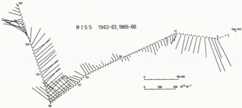
Fig. 13. Velocity vector changes along the traverse and reduced to unit length.

The velocity-change vectors around the traverse vertices, where the traverse angles differ considerably from 180°, enable us to determine the acceleration and curvature of the ice flow line at these points. The results are shown in Table II. According to this, r5 is slowed down considerably, but r17 still has a negative acceleration.