


Introduction
Many studies have been carried out to detect the equilibrium line and glacier facies using C-band synthetic aperture radar (SAR) with one polarization only (HH or VV). On large ice sheets it appears to be possible to detect different glacier facies (Reference Bindschadler and VornbergerBindschadler and Vornberger, 1992; Reference Fahnestock, Bindschadler, Kwok and JezekFahnestock and others, 1993; Reference PartingtonPartington, 1998), while many studies on smaller glaciers suggest that the equilibrium line can be detected (Reference Hall, Williams and SigurðssonHall and others, 1995; Reference Engeset and WeydahlEngeset and Weydahl, 1998). However, most of these studies lack ground observations, and recent work suggests that in many cases these studies have identified the firn line rather than the equilibrium line (personal communication from F. Rau and D. K. Hall, 1999). We define the firn line as the boundary between glacier ice and old firn from many previous years. The snowline, in contrast, is the lowest extent of the accumulated snow from the present mass-balance year at the end of the ablation season. The snowline usually approximates the equilibrium line. Some authors, in contrast to our definition, use the terms firn line and snowline interchangeably.
An example of the situation can be found on Kongsvegen glacier, Svalbard. Reference Engeset and WeydahlEngeset and Weydahl (1998) studied Kongsvegen using a European Remote-sensing Satellite (ERS) SAR image, and found excellent agreement between the equilibrium-line altitude (ELA) and an observed boundary on the SAR image. Reference EngesetEngeset (2000), however, looked at an 8 year time series of SAR images on the same glacier and found that this apparent agreement was accidental. The observed boundary occupied the same position year after year, and Reference EngesetEngeset (2000) concluded that this line represented the average firn-line altitude (FLA). Similarly, Reference Hall, Williams, Barton, Sigurðsson, Smith and GarvinHall and others (2000) found on Hofsjökull, Iceland, that the firn line may obscure the equilibrium line. Further information on these and other studies can be found in Reference Konig, Winther and IsakssonKönig and others (2001).
Glacier studies using multipolarization SAR (X-, C- and L-band) have been carried out in the Austrian Alps using the airborne NASA AIRSAR (Reference Rott and DavisRott and Davis, 1993; Reference RottRott, 1994; Reference Shi, Dozier and RottShi and others, 1994; Reference FloricioiuFloricioiu, 1997) and the Spaceborne Imaging Radar SIR-C/X-SAR on the space shuttle (Reference Rott, Nagler and FloricioiuRott and others, 1995). Similar to the findings of Reference EngesetEngeset (2000), Reference Rott and DavisRott and Davis (1993) report that polluted firn from previous years appeared below the present year’s snow on Système probatoire pour l’observation de la terre (SPOT) visible imagery acquired 1 day after the AIRSAR images. For mass-balance purposes, firn and snow need to be discriminated, but SAR cannot usually distinguish these two surfaces (Reference FloricioiuFloricioiu, 1997). The firn in the Alps, however, did not cover significant areas compared to snow (Reference FloricioiuFloricioiu, 1997).
Based on the above, we will examine our findings on Austre Okstindbreen, Norway, mainly in order to determine whether the firn line or the equilibrium line is visible on SAR imagery.
Motivation
In this section we explain why doubt has been cast on the ability of SAR to detect the equilibrium line. A comparable description can be found in Reference EngesetEngeset (2000), although here we consider a case without a superimposed-ice zone. Figure 1 presents a simplified cross-section of a glacier at the end of the ablation season. If we assume that no superimposed-ice zone exists, which is valid for most temperate glaciers, the present year’s equilibrium line is equal to the present year’s snowline at the end of the ablation season. In an ideal case, as illustrated in Figure 1a, the snowline divides the snow from the bare ice. From this we would assume that the late-summer snowline, i.e. the equilibrium line, can be easily identified on SAR images, since on winter images the smooth bare-ice facies results in low backscatter, while the snow facies gives a high backscatter (Reference Bindschadler and VornbergerBindschadler and Vornberger, 1992; Reference Fahnestock, Bindschadler, Kwok and JezekFahnestock and others, 1993). This is the situation assumed in many previous studies. The scenario just described, however, develops on top of previous years’ surfaces. Therefore, we can encounter two additional scenarios, which are also illustrated in Figure 1.

Fig. 1. Simplified cross-section of a glacier near the equilibrium-line location, with the late-summer snow cover of the present year on top. Three possible cases are drawn, showing the equilibrium line (a) at the same altitude as the firn line, (b) above the firn line and (c) below the firn line. Note the resulting SAR backscatter and that firn and snow can be indistinguishable due to similar backscatter.
In Figure 1b, we have a year with a mass balance that is more negative than average, and the late-summer snowline lies higher than the old firn line. In this scenario, we will not be able to see the present year’s equilibrium line, since the firn from previous years and the snow from the present year will both have a similar, high backscatter (Reference EngesetEngeset, 2000). We will, however, be able to see the firn line created by the old layers.
In Figure 1c, we have a mass balance which is more positive than average, and the late-summer snowline is located below the firn line. Here we can expect that either (1) the snow from the present year hides the firn line and has such high volume scattering that only the lower-lying snowline is visible on the SAR images, or (2) the present year’s snow layer has low volume scattering, in which case it is invisible in the SAR signal and only the firn line is visible.
The best acquisition time for the SAR images is during the winter following the mass-balance year. The dry winter snow-cover is normally invisible to the SAR signal, which has a penetration depth of tens of metres for dry snow at C-band (Reference MatzlerMätzler, 1987). The situation in the previous mass-balance year, as it appeared in late summer, is thus preserved in the SAR images. It must be ascertained that no melting has occurred before or during SAR acquisition. Just a slight amount of water or frozen ice lenses will alter the backscatter and thus obscure the late-summer situation we wish to observe (Reference Fahnestock, Bindschadler, Kwok and JezekFahnestock and others, 1993; Reference Rott, Nagler and KaldeichRott and Nagler, 1993).
Study Site and Data
Austre Okstindbreen is located in Norway (Fig. 2) at 66°01′ N, 14°18′ E. The total area of the glacier is 14 km2, and its elevation is about 730–1700 m a.s.l. (Fig. 2). A heavily crevassed icefall extends between about 1000 and 1200 m a.s.l., having an average slope of about 18°. The glaciers in the Okstindan area have been the focus of a cooperative project between the University of Manchester, U.K., and the University of Aarhus, Denmark, since 1970 (Reference KnudsenKnudsen, 1995b). Since 1976, the studies have concentrated on Austre Okstindbreen. Mass balance was measured between 1985 and 1996 (Reference KnudsenKnudsen, 1994, Reference Knudsen1995a, Reference Knudsenb). Six out of the nine years before 1996 had a positive balance. Generally, however, the glacier has been retreating for the last century and is now 2 km shorter than in 1908 (Reference Jacobsen and TheakstoneJacobsen and Theakstone, 1997). Field observations were made during the overflight of the Electromagnetic Institute of the Technical University of Denmark’s EMISAR and have been published in part in Reference Theakstone, Jacobsen and KnudsenTheakstone and others (1999).
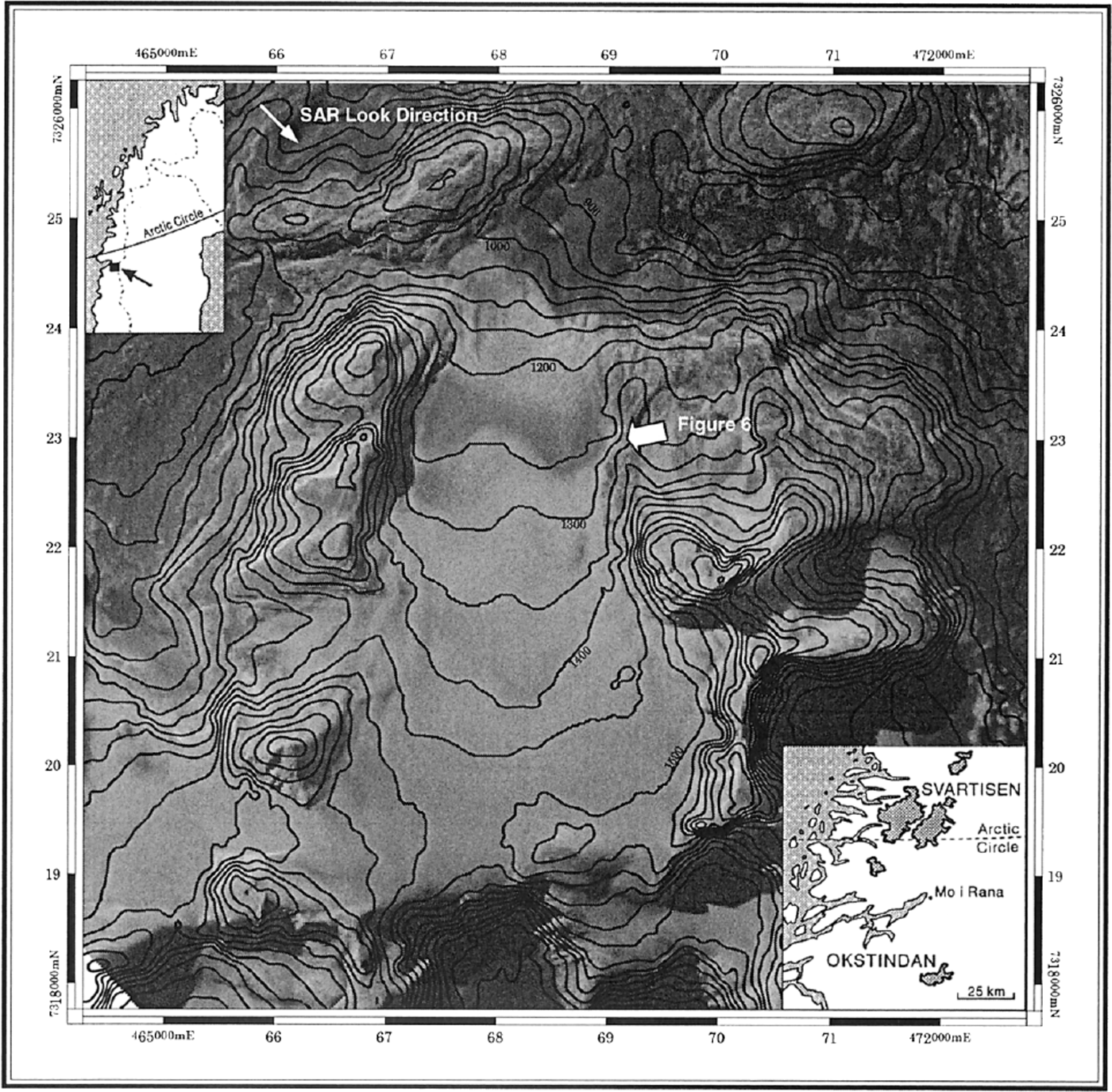
Fig. 2. The location of Austre Okstindbreen and the glacier as seen by the C-band HV-polarization image (23 March 1995) with elevation lines at 50 m intervals. The arrow marks the view direction of the photograph in Figure 6.
In spring 1995, the European Multisensor Airborne Campaign EMAC ’95 collected SAR images on 23 March (as well as 1 May and 5 July, which we do not consider here) with the EMISAR sensor. EMISAR is an airborne, dual-frequency (C-band, 5.3 GHz, and L-band, 1.25 GHz), multipolarization SAR sensor (Reference ChristensenChristensen and others, 1998). The incidence angle of the SAR signal is 35–65°. For a flat surface along the centre line of Austre Okstindbreen, the incidence angle varies only between 51.6° at the glacier tongue and 58.4° in the upper parts. The raw SAR images have been calibrated and geocoded by NORUT-Information Technology Ltd, Tromsø, Norway, using an algorithm described in Reference Johnsen, Lauknes and GuneriussenJohnsen and others (1995). The pixel size of the SAR images was resampled to 20 m during the calibration process. A digital elevation model (DEM) from the Norwegian mapping authority, Statens Kartverk, has been used for geocoding. It has a grid size of about 100 m with an accuracy of ±20 m elevation, and has been resampled to a grid size of 20 m for geocoding. A more detailed and more recent DEM has been developed for Austre Okstindbreen (Reference Theakstone and JacobsenTheakstone and Jacobsen, 1997), but this was not available at the time of geocoding. A detailed discussion of the accuracy of the geocoding process is provided below.
Observations and Image Analysis
The SAR images are presented in Figure 3, with a more detailed version of the C-band HV-polarization image in Figure 2. Figure 4 shows the backscatter along the centre line of Austre Okstindbreen. As a first observation we note that HH and VV backscatter are similar in both C- and L-band (see Fig. 4). The cross-polarization images HV and VH should be identical from SAR theory (Reference Ulaby and ElachiUlaby and Elachi, 1990), and differences in Figure 4 are probably due to radar system noise and calibration uncertainties. In both C- and L-band, the cross-polarization images HV and VH contain more variation in backscatter than the HH and VV images (see Fig. 4). This is in agreement with Reference RottRott (1994), who found that the separation of snow and glacier ice is improved by using C-band cross-polarization data. The reason for this is that glacier ice, being a smooth surface, does not change the polarization of the incoming signal. Thus the return in the cross-polarized images is very low, lower than in the HH and VV images, and the glacier-ice areas are more easily recognized. The snow and firn contain snow crystals, leading to multiple scattering, which changes polarization of the incoming wave and causes cross-polarization images to have similar backscatter to HH and VV images.
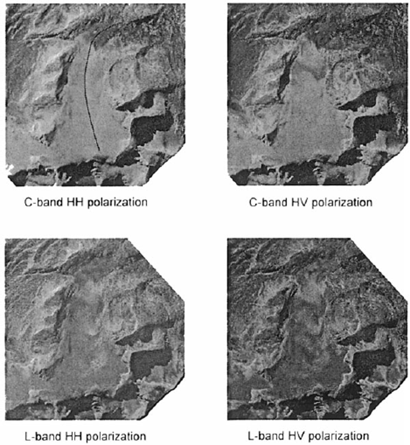
Fig. 3. The EMISAR images acquired for Austre Okstindbreen on 23 March 1995 in C- and L-band with different polarizations. VH- and VV-polarization images are not shown, since they look the same as HV- and HH-polarization images, respectively. The centre line used to extract backscatter values (see Fig. 4) is marked in black in the C-band HH-polarization image.
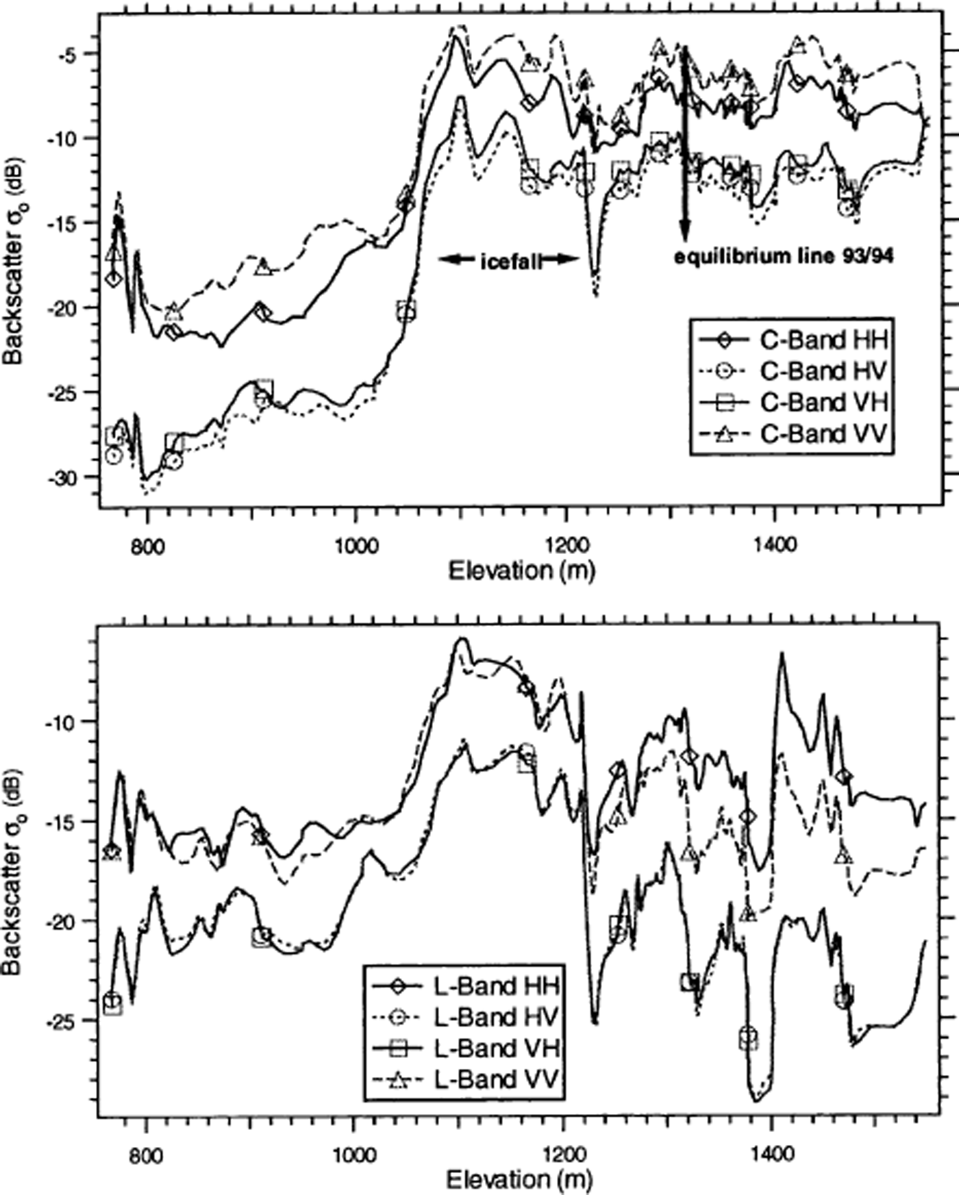
Fig. 4. Backscatter along the centre line (see Fig. 3) of Austre Okstindbreen for C- and L-band in all available polarizations. Binomial smoothing was applied to the raw data. The high backscatter of the icefall can be seen at about1050–1220 m a.s.l. A distinct increase in backscatter at 1230 m a.s.l. is seen in HV and VH polarization. The incidence angle of EMISAR for a flat surface along this centre line varies between 51.6° at the glacier tongue and 58.4° in the upper parts.
L-band penetrates deeper into the glacier and reveals, for example, crevasses and the bergschrund in the accumulation area, which are not seen in C-band (Fig. 3). Field observations show little or no evidence of these crevasses on the glacier surface, and snow-probing reveals that many of them are buried by several metres of snow. In the following we will concentrate on the C-band images, and especially on the C-band HV polarization (Fig. 2), where most variation is seen.
Reference Rott, Nagler and FloricioiuRott and others (1995) reported backscatter values from multipolarization SIR-C/X-SAR from the Austrian Alps (see also Reference FloricioiuFloricioiu, 1997). These images, like ours from Austre Okstindbreen, were acquired in spring before the beginning of snowmelt. For the glacier ice area < 1000 m a.s.l. our values agree with those of Reference Rott, Nagler and FloricioiuRott and others (1995) in L-band, but are about 5 dB lower in C-band. L-band penetrates into the glacier ice and we assume that similar values in both studies are due to the similar structure of the glacier ice. C-band, on the other hand, is dominated by scattering at the snow–ice interface below the dry winter snowpack (Reference Rott, Nagler and FloricioiuRott and others, 1995), and lower values in our case suggest a comparably smoother glacier surface at Austre Okstindbreen. For the firn areas, our values are in agreement with those of Reference Rott, Nagler and FloricioiuRott and others (1995) in C-band, and they are about 5 dB lower in L-band. This suggests similar snow characteristics of the snow cover in both cases, while higher backscatter in the deeper-penetrating L-band suggests relatively larger grain-sizes or possibly ice lenses deeper in the Alpine firn, whose presence is reported in Reference Rott, Nagler and FloricioiuRott and others (1995). The standard deviation of L-band backscatter at Austre Okstindbreen, however, is quite large (about 3 dB), and parts of the glacier exhibit L-band backscatter values comparable to those reported by Reference Rott, Nagler and FloricioiuRott and others (1995). Again, insufficient field data are available for Austre Okstindbreen to check our assumptions against ground truth.
Radar backscatter depends strongly on the incidence angle of the radar beam (Reference Rott, Nagler and FloricioiuRott and others, 1995). ERS SAR satellites have a much lower incidence angle than EMISAR (23° vs 51.6–58.4° for the centre line of Okstindbreen), and backscatter values will therefore be considerably higher for ERS SAR images. However, relative differences between firn and glacier-ice areas in the studies by Reference PartingtonPartington (1998) and Reference EngesetEngeset (2000) are comparable to our results. Backscatter differences for incidence angles of 50–60° are relatively small (Reference Rott, Nagler and FloricioiuRott and others, 1995), so we assume a negligible effect on the backscatter for Austre Okstindbreen.
Low backscatter is seen on the glacier tongue (Figs 2 and 4a). The smooth glacier ice surface does not reflect much energy back to the SAR sensor. At higher elevations in the glacier bend, at about 1050–1200 m a.s.l., we find an area of high backscatter. In this zone, there is a large icefall with a highly crevassed and rough surface that reflects much of the SAR signal and leads to high backscatter. At about 1220–1250 m a.s.l., we again find low backscatter, more distinct in the HV than in the HH polarization. Snow-pit data at 1230 m a.s.l. from Reference KnudsenKnudsen (1995b) show a smooth glacier ice surface, and Reference Theakstone, Jacobsen and KnudsenTheakstone and others (1999) report that glacier ice is exposed towards the end of the ablation period in this area.
At around 1250 m a.s.l. we find a distinct boundary on the C-band images, above which the backscatter is considerably higher, especially in the cross-polarization images. On the L-band images, this boundary is seen only weakly (Fig. 3), and, in contrast to C-band, there is not much backscatter difference between the lower and upper glacier. Only the icefall appears distinct in both L- and C-band. In the rest of this paper we analyze the nature of this boundary, which we call the 1250 m line (noting that it only approximately follows the 1250 m contour line and that parts of it are at somewhat higher or lower elevations). We suggest that similar SAR boundaries have been interpreted as the equilibrium line but may actually be the firn line.
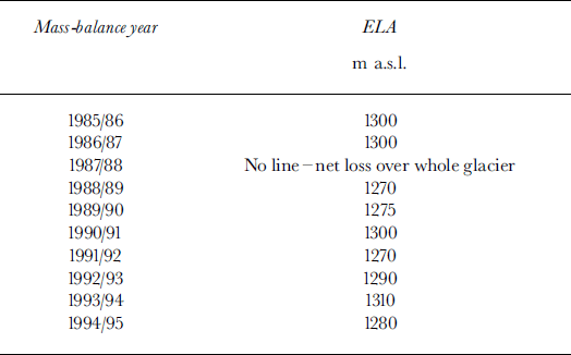
We can immediately see that the 1250 m line is not equivalent to the 1993/94 equilibrium line, which is located at 1310 m a.s.l., and is about 700 m away from the 1250 m line along the glacier’s centre line (Reference KnudsenKnudsen, 1995a). The 1250 m line is also situated lower than any equilibrium line since 1985/86, the lowest such line being 1270 m in 1988/89 (Table 1). The average ELA for the years 1985–94 is 1290 m a.s.l.
Table 1. ELA, 1985–94
Reference Elvehøy, Haakensen, Kennett, Kjøllmoen, Kohler and TvedeElvehøy and others (1997) and Reference Theakstone, Jacobsen and KnudsenTheakstone and others (1999) report a distinct increase in snow depth from 1 to 2 m snow water equivalent between about 1250 and 1300 m a.s.l. (Fig. 5). We can expect from theory that the dry winter snow cover is invisible to the SAR due to the large penetration depth of the microwave signal (Reference MatzlerMätzler, 1987). Nonetheless, we examine whether the 1250 m line may be due to this strong increase in winter snow thickness, which coincides with the location of the 1250 m line. The transect at about 1230 m a.s.l. in Figure 5 shows that the snow depth is high at the sides of the glacier and lower around the centre line. This is consistent with observations on many glaciers (e.g. Reference Winther, Bruland, Sand, Killingtveit and MarechalWinther and others, 1998) and is due to deposition of drifting snow along the glacier margin, but it is the opposite of what we would expect from the shape of the 1250 m line. Assuming dependence of the SAR signal on snow depth, the low backscatter on the sides would require a low snow depth, such that the SAR signal was reflected by the glacier ice. The high backscatter at the centre line would require high snow depth such that volume scattering was possible. Since we observe the opposite distribution to what would be required, in addition to the large penetration depth of SAR in dry snow (Reference MatzlerMätzler, 1987), we conclude that the 1250 m line is not due to the 1994/95 winter snow-depth distribution.
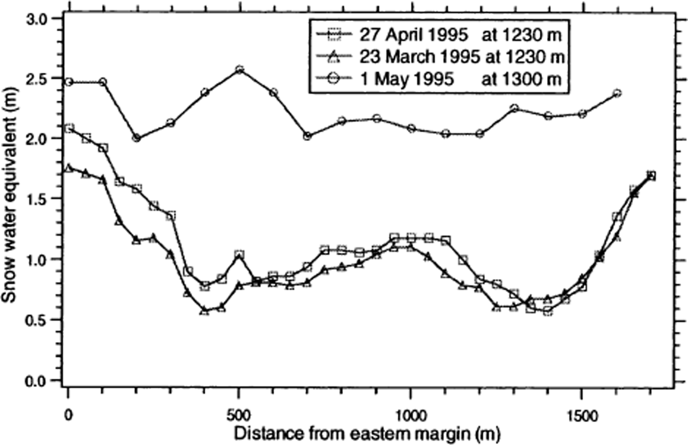
Fig. 5. Two transects on Austre Okstindbreen perpendicular to the centre line, one at 1230 m a.s.l., the other two at approximately 1300 ma.s.l.
Evidence on the nature of the 1250 m line can be found on a photograph from August 1995 (Fig. 6), whose view direction is marked in Figure 2. The snowline, i.e. the equilibrium line, was at 1280 m at the end of the balance year (Reference KnudsenKnudsen, 1995b), but in early August 1995 it was still close to 1250 m. In 1994, the year represented by the SAR images (Figs 2 and 3), the late-summer snowline was much higher at about 1300 m. Below the snowline from August 1995 is the old firn (Fig. 6). The firn line, i.e. the boundary between firn and ice, in Figure 6 has the same shape as the 1250 m line on the SAR images.

Fig. 6. A photograph from August 1995 showing snow and firn line of Austre Okstindbreen at around 1250 m a.s.l. The location and view direction of this photograph is marked in Figure 2. The flow direction of the glacier is to the right, and crevasses from the upper end of the icefall can be seen. The firn line follows the same shape as the 1250 m line in Figure 2. The snowline, which was located at 1250 m in August 1995, was much higher at about 1300 m in August 1994, i.e. the year represented by Figure 2.
The shape of the 1250 m line suggests that it has been affected by glacier movement. It is further down the glacier around the faster-flowing centre line and further up the glacier at the slower-flowing sides of the glacier. We therefore conclude that the 1250 m line is the firn line created by previous years’ layers, which is deformed by the ice movement. We thus have the case described in Figure 1b with an equilibrium line at higher elevation and a lower-lying firn line. In the following we will model the stratigraphy of Austre Okstindbreen as an additional way of determining FLA.
Modelling the Stratigraphy
We know from field observations documented in Figure 6 that the 1250 m line is the firn line created by old layers of firn from several previous years. In order to understand the firn line’s development, we have written a simple algorithm that models the stratigraphy of Austre Okstindbreen from previous years’ net balance data. A cross-section of the glacier reveals a stratigraphy in the accumulation area, consisting of previous years’ layers of accumulated snow. Each year a layer of snow is deposited and then buried by the following year’s snow accumulation. In addition, glacier movement transports the layer further down-glacier. To derive the position of the firn line, we model the stratigraphy of Austre Okstindbreen using the available information on mass balance from 1986 to 1994 (Reference KnudsenKnudsen, 1994, Reference Knudsen1995a). The steps of the algorithm are as follows:
-
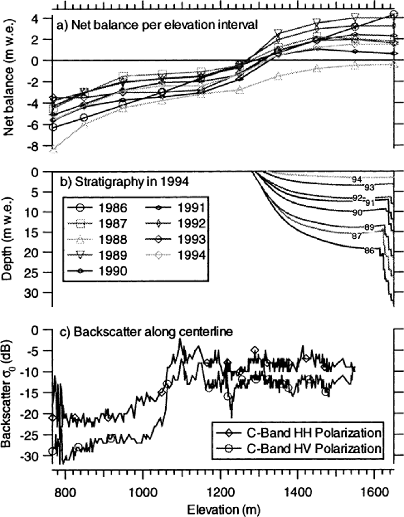
(a) The curves in Figure 7a represent the net balance on Austre Okstindbreen for the years 1986–94. These curves are based on a large number of snow measurements on the glacier, which were averaged into a net balance value for each 100 m elevation interval on Austre Okstindbreen. We interpolate this curve in order to obtain a net balance value for every point along the x axis.

Fig. 7. (a) Met balance curves, 1986–94. (b) Modelled stratigraphy; every line represents the lower boundary of that year’s layer. (c) Centre-line backscatter; the deviation between the modelled firn line at 1280 m and the backscatter increase at 1230 m is due to inaccuracy of the model and georegistration errors.
-
(b) Using this net balance information, we wish to model a certain year’s surface as it appears in a later year. We want to follow, for example, the 1986 layer from its deposition in 1986 through its different stages up to the location where we would observe it in 1994. The net balance curve for 1986 can be seen in Figure 7a. Any negative value of the 1986 net balance curve means that snow or ice at this location has melted away and thus no 1986 surface is visible at this location. At the remaining points, where the net balance is positive, snow is being deposited, creating a 1986 layer.
-
(c) In the following year, the 1986 layer is first moved towards the glacier tongue due to the glacier velocity. We assume movement parallel to the glacier surface, which is valid around the equilibrium line, and use the centre-line velocities close to the equilibrium line. These velocities were derived in the field from stake surveys as reported by Reference KnudsenKnudsen (1994, Reference Knudsen1995a). After the 1986 layer has been moved, it is affected by the present year’s net balance from Figure 7a. This moves the 1986 layer deeper into the glacier where this year’s net balance is positive, and closer to the surface at locations where this year’s net balance is negative. At locations where the net balance is especially negative, the 1986 layer may be melted away and vanish. Step (c) is repeated for each of the following years 1987–94, moving the 1986 layer according to glacier velocity and net balance. The final location of the 1986 layer in 1994 can be seen in Figure 7b.
-
(d) Steps (b) and (c) are repeated for each of the annual layers from 1986 to 1994. The resulting stratigraphy can be seen in Figure 7b. Each layer in this graph (e.g. the line representing the 1986 layer) represents the base or deepest point of this layer at a certain elevation.
Comparing Modelled and Visible Line
Figure 7b shows the results from the modelled stratigraphy. Here, the firn line is located at 1282 m a.s.l. at the centre line, while Figure 7c shows that the 1250 m SAR line is at 1230 m a.s.l. at the centre line. In terms of ground distance the 1250 m line and the firn line are separated by 500 m. The question remains whether according to the model the 1250 m line is indeed the firn line. Possible errors in the analysis, which could cause this 500 m deviation, are as follows:
During the process of geocoding, each pixel of the SAR image is tied down to its corresponding location on a DEM. The DEM thus serves as the basis for georegistration. The accuracy in location of any SAR pixel depends therefore on two factors: the accuracy of the map base, i.e. the DEM, and the accuracy of tying a certain SAR pixel to its real location on the DEM.
The accuracy of the DEM used is ±20 m elevation according to the producer of the DEM, Statens Kartverk. The elevation of any SAR pixel therefore cannot be determined to better than ±20 m elevation, assuming that each SAR pixel has been assigned to its accurate location on the ground (i.e. latitude and longitude).
To find the accurate geolocation of a SAR pixel, some easily recognizable features, such as mountain tops, are used as tie points, while the location of the remaining points is calculated as described in Reference Johnsen, Lauknes and GuneriussenJohnsen and others (1995). This calculation inevitably leads to errors. Using control points after georegistration, we found that the deviation between DEM location and SAR pixel location is usually 100–200 m ground distance. This is not surprising since the DEM originally had a grid spacing of 100 m and was resampled to a 20 m grid. The largest observable deviation can be seen in Figure 2 in the lower right corner of the glacier. The contour lines of the mountainside and the SAR image deviate here by 350 m ground distance. A pixel location of the SAR image can thus deviate from its real position by 100–350 m ground distance, which corresponds to about 10–30 m error in elevation in the area of the 1250 m line. If we thus consider inaccuracy of the DEM and georegistration errors, we estimate an accuracy of ±40 m elevation for a SAR pixel in the area close to the equilibrium line.
On the other hand, we have an inaccuracy of the modelled FLA. The algorithm uses net balance data averaged over 100 m elevation bands. The strong increase in snow depth at 1250 m in every year, as reported in Reference Elvehøy, Haakensen, Kennett, Kjøllmoen, Kohler and TvedeElvehøy and others (1997) and Reference Theakstone, Jacobsen and KnudsenTheakstone and others (1999), suggests that the net balance curves in Figure 7a may be steeper and cross the zero line at lower elevations. This would cause the firn line to be located lower than in Figure 7b. The use of inaccurate velocity values can be neglected as an error source. According to the model, the FLA is relatively insensitive to velocity changes, and a greatly different velocity would be needed to give a significant change in FLA.
Considering these points, modelled FLA and the visible 1250 m line lie very well within the error margins. We can therefore justify the assumption that the 1250 m line is indeed the firn line and that the observed discrepancy between Figure 7b and c is due to the inaccuracy of the methods used. This is supported by the fact that we can confidently exclude other possible explanations for the 1250 m line, such as a strong increase in snow depth or the 1995 equilibrium line, whose 1310 m elevation is too far from the visible 1250 m line.
Conclusions
Our study suggests that multipolarization SAR, like the future ASAR or RADARSAT-2, will be a better tool for glacier monitoring than previous single-polarization SAR sensors. Cross-polarization SAR images (HV and VH) display a greater variation in backscatter than HH and VV polarization and reveal more details of the glacier surface. C-band is preferred for mass-balance observations; L-band penetrates much deeper and can be used to detect crevasses buried by snow and firn.
The snowline from the end of the ablation season, approximating the equilibrium line, could not be detected with the SAR data; a distinct boundary was visible on the glacier, however, which we conclude from photographic evidence to be the firn line created by previous years’ snow layers. Additionally, modelled FLA and the observed line are separated by 50 m elevation, but considering errors during co-registration and modelling, this is not a significant difference.
Monitoring of the firn line will be a valuable source of information. The firn line is not itself affected by yearly variations in ELA, but a permanent change in the average ELA will eventually result in a change in FLA. The firn line therefore seems to smooth out short-term variations and to show trends on a longer time-scale. The FLA thus serves as a valuable climate indicator and appears to be easily detectable on SAR images due to strong difference in backscatter between ice and firn. This suggests that the connection between FLA and mass balance needs to be studied further so that SAR can be used for routine mass-balance observations. Eventually, this may call for the development of correlation factors between FLA and mass balance, in contrast to today’s use of ELA, in order to use SAR for routine mass-balance monitoring.
Acknowledgements
We wish to thank I. Lauknes from NORUT-Information Technology Ltd, Tromsø, who did the geocoding of the SAR images. Discussions with R. Engeset (Norges Vass-dragsog Energiverk, NVE, Oslo) and J. Kohler (Norsk Polarinstitutt, Tromsø) provided helpful insights. Thanks go also to W. H. Theakstone (University of Manchester) for information on Austre Okstindbreen. This project is funded by the European Space Agency and the Norwegian Space Centre (PRODEX Implementation Contract No. 13505/99/NL/VJ(1C)) and the Norwegian Polar Institute (NP).


