


1. INTRODUCTION
Glacier mass balance is directly influenced by fluctuations in local weather and climate. Global warming has drawn the attention of glaciologists owing to its strong impact on glacier change (e.g., Braithwaite and Yu, Reference Braithwaite and Yu2000; Kang and others, Reference Kang2010; Marzeion and others, Reference Marzeion, Jarosch and Hofer2012; Radić and others, Reference Radić2013). The accumulation and ablation of glaciers are not only related to air temperature and precipitation but also other variables such as debris cover, cloudiness, surface impurities, wind, humidity, radiation, surface slope and aspect. Incoming shortwave radiation (S ↓) and longwave radiation (L ↓) are key variables in the energy balance (e.g. van den Broeke and others, Reference van den Broeke, Ettema and Munneke2008; Yang and others, Reference Yang2011; Sun and others, Reference Sun2012; Zhang and others, Reference Zhang2013; Sun and others, Reference Sun2014; Cullen and Conway, Reference Cullen and Conway2015). Accurate estimates of these variables are needed when modeling glacier surface energy and mass balance.
Clouds can alter the magnitude and nature of S ↓from shortwave radiation incident at the top-of-atmosphere and increase the proportion of diffuse radiation. Similarly, clouds can dramatically enhance the ability of the atmosphere to radiate longwave radiation. Clouds are very frequent in many high-altitude mountainous regions and the cloud/radiative interactions there are very complex, owing to low temperatures and water vapor content, the presence of the highly reflective and inhomogeneous snow/ice surfaces and multilayered clouds. Some works have shown that over maritime glaciers, cloud tended to increase Rnet (the sum of net shortwave radiation (Snet) and net longwave radiation (Lnet); van den Broeke and others, Reference van den Broeke, Ettema and Munneke2008; Gillett and Cullen, Reference Gillett and Cullen2011). Incorrect understanding of cloud/radiative interactions may result in misunderstanding of climate and earth surface interaction. For example, Arctic sea-ice extent reached a minimum during summer 2007, to which Kay and others (Reference Kay, L'Ecuyer, Gettelman, Stephens and O'Dell2008) believed that reduced cloud fractions and enhanced S ↓contributed. However, Schweiger and others (Reference Schweiger, Zhang, Lindsay and Steele2008) illustrated that the increase of S ↓ from reduced cloud fractions contributed little to that 2007 minimum. Moreover, magnitudes of other meteorological variables vary with cloud cover. Conway and Cullen (Reference Conway and Cullen2016) showed that relative humidity was always higher on overcast days than on clear-sky days; while air temperature was lower, the surface temperature was higher on overcast days during the warm season. Therefore, detailed knowledge of the effects of clouds on glacier melt is very important.
The Qilian Mountains act as the water source for Hexi Corridor in China. In winter, there is a dry, rainless continental climate under control of the Mongolian high. In summer, the upper atmosphere over the Bay of Bengal and Tibetan Plateau (TP) is a heat source (Long and Li, Reference Long and Li1999) and the Mongolian high weakens, allowing southwesterly airflow to bring moisture from the Indian Ocean and the Bay of Bengal to Hexi Corridor. This airflow can occasionally transport moisture as far as the western Qilian Mountains, while an intense Mongolian cyclone causes a strong meridional wind that blocks Arctic air masses from reaching Hexi Corridor (Du and others, Reference Du, Qin, Kang, Cui and Sun2016). Several studies of glacier energy and mass balance have been carried out in the Qilian Mountains (Jiang and others, Reference Jiang, Wang, He, Wu and Song2010; Sun and others, Reference Sun2012, Reference Sun2014), but did not address the effects of cloud cover on glacier melt.
Most studies of cloud effects focused on maritime or Arctic glaciers (e.g., Greuell and others, Reference Greuell, Knap and Smeets1997; Gillett and Cullen, Reference Gillett and Cullen2011; Pellicciotti and others, Reference Pellicciotti, Raschle, Huerlimann, Carenzo and Burlando2011; Conway and Cullen, Reference Conway and Cullen2016; Sicart and others, Reference Sicart, Espinoza, Quéno and Medina2016; Van Tricht and others, Reference Van Tricht2016), but little is known about the effects on continental and high-elevation glaciers. This paper addresses these issues using observed meteorological variables and glacier melt data from three automatic weather stations (AWSs) at Laohugou glacier No. 12. The radiative properties of clouds were investigated through their shortwave transmissivity and longwave emissivity. Combined with the AWS observations, the cloud effects on radiation and meteorological variables and glacier melt were quantified.
2. SETTING AND AWS DESCRIPTION
Laohugou glacier No. 12 (Fig. 1) is a mountain glacier in the upper Shulehe River basin of the western Qilian Mountains, northeast TP, and is the largest glacier in the Qilian Mountains. The glacier faces northwest, is 9.85 km long, and has a total area of 20.4 km2. Its elevation ranges from 4260 m to 5481 m a.s.l. (Du and others, Reference Du, Qin, Liu and Wang2008). The lower part of the glacier (below 5000 m a.s.l., 52% of its total area) is relatively steep and the upper part (48% of the total area) is wide and flat (3°–6°) with a 480 m altitude difference. Annual precipitation was 310 mm w.e. during 1960–2006 (Qin and others, Reference Qin2015) and the annual air temperature was −13.2°C during 1957–2013 (Qin and others, Reference Qin2014) at 5040 m a.s.l. The glacier has experienced pronounced thinning and areal reduction in past decades; from 1957 to 2007, ice thickness decreased by 18.6 m and surface area by 0.82 km2 (Zhang and others, Reference Zhang, Liu, Shangguan, Li and Zhao2012).
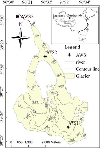
Fig. 1. Map of Laohugou glacier No. 12 showing AWS locations. Contour are at 100 m intervals.
The three AWSs used were AWS1, AWS2 and AWS3 (Fig. 1). AWS1 (5040 m a.s.l.) and AWS2 (4550 m a.s.l.) were installed on the glacier and AWS3 (4190 m a.s.l.) was located in a meadow 1.6 km from the glacier terminus. Precipitation was measured in mm w.e. using a Geonor T-200B gauge, which is an accumulative weighing bucket-type precipitation gauge without heating, on the eastern margin of the glacier at the same elevation as AWS2. The stations were of identical design. Table 1 gives details of the instrumentation of the three AWSs and a rain gauge. All sensors were connected to a data logger (CR1000, Campbell, USA) which had low-temperature resistance. The logger was configured to store half-hourly means of measurements taken every 10 s. AWS1 and AWS2 were installed on the glacier surface using a steel tripod, with wood blocks of size 70 cm × 70 cm placed under each tripod leg to provide stability and prevent melting of the tripod legs into the ice. The AWSs were placed on a relatively flat surface. The base of AWS1 was always covered by snow or ice, preventing tilt caused by melt at the bottom of the AWS. During the glacial melt period (June–September), AWS2 was visited every 3–5 days, and AWS1 about once per month. Although the AWS tilted because of glacier melt, the weekly checks kept the instrument largely parallel to the glacier surface. Data were collected from 1 January 2011 to 31 December 2012.
Table 1. AWS technical parameters and sensor installation heights
3. METHODS
3.1. Data treatment
During morning and evening, when the solar angle is low, the downward shortwave radiation (S ↓) is occasionally less than upward shortwave radiation. Data with S ↓<10 W m−2 were discarded. To avoid the effect of low solar elevation on albedo, albedos between 12.00 and 16.00 hours were averaged to daily resolution. Measured precipitation was corrected following the method of Ma and others (Reference Ma, Zhang, Yang and Farhan2015) to account for undercatch caused by wind-induced error, wetting loss and evaporation. The air temperature sensor was installed inside a ventilated radiation shield.
3.2. Mass balance
Surface height change measured by sonic range sensor was converted into specific mass balance according to the following method. Derived daily surface height changes at AWS1 and AWS2 were converted into w.e. thicknesses according to the daily albedo value, as follows. Increases in surface height (accumulation) were multiplied by 0.3, which was the observed average new snow density. Sampled accumulation during June–September was then distributed over the entire glacier using 100 m elevation bins. For decreases in surface height (ablation), the surface height change was multiplied by 0.9 (the ice density) if the daily mean albedo was <0.4 (Cutler, Reference Cutler1996), or multiplied by 0.5 if the albedo was between 0.4 and 0.7, corresponding to the observed average density 0.5 g cm−3 in the snow pit adjacent to AWS1 measured during July.
Nine plastic stakes were installed near AWS2 (Sun and others, Reference Sun2014) and one near AWS1. The stakes were measured every 3–5 days at AWS2 and ~1 month at AWS1 during summer 2011. These measurements were used to validate the mass balance recorded by sonic range sensor.
3.3. Longwave radiation model
L ↓ is governed by the Stefan–Boltzmann law:
 $$L_ \downarrow = \varepsilon _{{\rm eff}} {\rm \;} \sigma {\rm \;} T_{\rm a}^4, $$
where T a is air temperature in the near-surface layer (k) and ε eff is the effective emissivity of the atmosphere. During clear skies, the variation of effective emissivity (ε cs) is controlled by the profile of air temperature and water vapor pressure (e, hPa) at screen level. ε cs is parameterized following Konzelmann and others (Reference Konzelmann, van de Wal, Greuell and Abe-Ouchi1994).
 $$\varepsilon _{{\rm cs}} = \varepsilon _{{\rm ad}} + p^1 ({\rm e}_{\rm a} /T_{\rm a} )^{(1/p^2 )}, $$
where ε ad is the emissivity for a clear, dry atmosphere (ε ad = 0.22; (Dürr, Reference Dürr2004)). P 1 and p 2 are constants. p 2 was assigned a value from previous studies and p 1 was tuned using clear-sky incoming longwave radiation (L ↓M−cs) measured at AWS3.
Days with cloudless sky were selected following Conway and others (Reference Conway, Cullen, Spronken-Smith and Fitzsimons2015), which were identified on the basis of a monotonic increase of S ↓ during the morning and corresponding decrease during the afternoon. On some cloudy days, although S ↓ followed the above pattern, visual inspection clearly identified the effect of clouds, and these days were reclassified as cloudy. From the original 2-year dataset at AWS3, a total of 66 cloudless days were selected to optimize the clear-sky model.
In complex topography, L ↓ is reduced because part of the sky is obstructed, but additional radiation is received from surrounding slopes (Hock and Homgren, Reference Hock and Homgren2005). Received longwave radiation from these slopes is influenced by the effective temperature of surrounding terrain and the sky view factor. Sky view was calculated from a 30 m × 30 m DEM (http://datamirror.csdb.cn) according to the shadow casting algorithm of Lindberg (Reference Lindberg2005). Calculated values of F are 0.975 at AWS1, 0.97 at AWS2 and 0.911 at AWS3. Here, a simple scheme was used whereby the effective temperature of surrounding terrain is represented by T a. The final expression for L ↓ is
 $$L_ \downarrow = F\varepsilon _{{\rm eff}} {\rm \;} \sigma {\rm \;} T_{\rm a}^4 + \left( {1 - F} \right)\varepsilon _{{\rm eff}\_{\rm rock}} \sigma {\rm \;} T_{\rm a}^4 {\rm \;}, $$
where $\varepsilon _{{\rm eff}\_{\rm rock}} $
is the emissivity of rock (0.9).
$\varepsilon _{{\rm eff}\_{\rm rock}} $
is the emissivity of rock (0.9).
To quantify the influence of cloud on L ↓, longwave equivalent cloudiness was defined by van den Broeke and others (Reference van den Broeke, van As, Reijmer and van de Wal2004) as
 $$N_{\rm L} = (\varepsilon _{{\rm eff}} - \varepsilon _{{\rm cs}} )/(\varepsilon _{{\rm ov}} - {\varepsilon} _{{\rm cs}} )$$
 $$N_{\rm L} \left( {N_{\rm L} \gt 1} \right) = 1;{\rm \;} N_{\rm L} \left( {N_{\rm L} \lt 0} \right) = 0,{\rm \;} $$
where ε ov = 1 is emissivity in overcast conditions and ε eff is the actual effective emissivity, calculated by rearranging Eqn (1) for L ↓ = L ↓−M.
3.4. Shortwave radiation model
To quantify the influence of clouds on S ↓, a cloud transmission factor (trc) was used (Greuell and others, Reference Greuell, Knap and Smeets1997), defined as the ratio of S ↓−M to theoretical clear-sky radiation (S ↓cs):
 $$trc = S_{ \downarrow - {\rm M}} /S_{ \downarrow {\rm cs}}. $$
Some studies have defined trc as the ratio of S ↓−M to top-of-atmosphere shortwave radiation (S TOA) (Hock and Homgren, Reference Hock and Homgren2005; Sedlar and Hock, Reference Sedlar and Hock2009), but this includes effects of both cloud and clear-sky atmospheric attenuation. The basic equation to calculate S ↓cs is
 $$\; S_{ \downarrow {\rm cs}} = S_{{\rm cs}} + D_{{\rm cs}}, $$
where D cs is diffuse solar radiation and S cs is direct beam solar radiation, which is calculated as follows (Bird and Hulstrom, Reference Bird and Hulstrom1981):
 $$S_{{\rm cs}} = 0.9751S_0 E_0 {\rm sin}h{\rm \tau} _{{\rm cs}}, $$
where S 0 is the solar constant (1367 W m−2), E 0 the eccentricity correction factor, h the solar elevation above the plane of the horizon and τcs the clear-sky transmissivity of the atmosphere for the (broadband) direct sunbeam. The coefficient 0.9751 is the ratio of solar to extraterrestrial radiation. The term τcs includes the extinction of solar radiation by Rayleigh scattering (τr), absorption by gases (τg), absorption by water vapor (τw) and attenuation by aerosols (τa). The terms τr, τg and τa are calculated as functions of optical air mass and air pressure, and τw is estimated from optical air mass and precipitable water (Parta, Reference Parta1996). The total vertical column ozone value is 0.294 cm, based on the annual average for the entire TP (Zou, Reference Zou1996). τa varies with space and time, and is given by τa = x ma (e.g., Mölg and others, Reference Mölg, Cullen and Kaser2009; Conway and others, Reference Conway, Cullen, Spronken-Smith and Fitzsimons2015). Here, we defined x as the ratio of S ↓−M to predicted S ↓cs, excluding aerosol effects.
D cs comprises two components, one from clear sky and the other from reflected solar radiation from the surrounding terrain (D t). D cs from the sky is the sum of the contributions of Rayleigh scattering (D r), aerosol scattering (D a) and multiple reflections between the surface and atmosphere (D m):
 $$D_{{\rm cs}} = (D_{\rm r} + D_{\rm a} + D_{\rm m} )F + D_{\rm t} (1 - F),$$
where D t is calculated by
 $$D_{\rm t} = \alpha _{\rm t} S_ \downarrow. $$
Here, α t is the albedo of the surrounding terrain. AWS1 was in a firn basin and was always surrounded by firns, so α t was set to 0.7 (the measured fern albedo). AWS2 was in an ablation zone where glacier ice was always exposed, so α t was set to 0.4 as per the maximum for glacier ice suggested by Cutler (Reference Cutler1996). AWS3 was surrounded by rock, so a rock albedo of 0.18 (Klok and Oerlemans, Reference Klok and Oerlemans2002) was chosen. D cs from the clear sky (D r + D a + D m) was calculated following Bird and Hulstrom (Reference Bird and Hulstrom1981).
To quantify the influence of clouds on S ↓, shortwave radiation cloudiness (N S) was derived from a simple cloud metric (Mölg and others, Reference Mölg, Cullen and Kaser2009), which includes a cloud extinction coefficient (k) varying with geographic latitude:
 $$N_{\rm s} = (1 - trc)/k$$
 $$N_{\rm s} (N_{\rm s} \gt 1) = 1;{\rm \;} N_{\rm s} (N_{\rm s} \lt 0) = 0{\rm \;} {\rm.} $$
4. RESULTS
4.1. Air temperature and humidity
In the study region, air temperature followed a clear seasonal cycle. Annual mean air temperatures at all three sites were <0°C, but in melt season (May–September) the average air temperature at AWS3 was >0°C (Table 2). The mean temperature lapse rate between AWS1 and AWS2 was−6.1°C km−1, but the lapse rate was smaller during melt season (−4.9°C km−1). The lapse rate between the glacier and nonglacierized areas was much steeper owing to the glacier cooling effect, with an annual mean of −9.6°C km−1 between AWS2 and AWS3 and −7.6°C km−1 between AWS1 and AWS3. The daily mean air temperature was strongly correlated between the three AWSs sites (Table 2).
Table 2. Mean values of meteorological quantities and cloud cover
Measurements of relative humidity indicated dry conditions at Laohugou glacier No. 12, with annual mean relative humidity ~50% (Table 3). Relative humidity increased with altitude, except that between AWS1 and AWS2 during the melt period. The annual mean vapor pressure was ~2 hPa, reaching 3.6 hPa in summer.
Table 3. Correlation (R 2) and RMSE between measured and simulated half-hour, clear-sky incoming longwave radiation
4.2. Wind speed and direction
The wind speed was stronger in winter at AWS1 and AWS2, but varied little between summer and winter at AWS3 (Table 2). The correlation was moderate between AWS1 and AWS2, but correlations were insignificant between the glacier site and nonglacier site, where R 2 was as small as 0.28 between AWS1 and AWS3.
Dominant wind directions varied between the AWSs. AWS1 was in a wide fern basin, with little shelter from the prevailing westerly wind and little influence from katabatic winds. AWS2 and AWS3 were in a narrow valley, which provided shelter from the westerlies. Katabatic winds were more frequent at both lower sites, with directions parallel to the valley orientation; at AWS2, the west and east branches of the glacier converge and flow northward, whereas the valley at AWS3 has an orientation of ~135°.
4.3. Incoming longwave radiation and N L
L ↓ decreased with altitude because of the decrease in air temperature, with a mean gradient of −36 W m−2 km−1. Daily mean L ↓ values at the three AWS sites were also strongly correlated (Table 2). In summer, high air temperature and more frequent cloud cover increased L ↓ by ~50 W m−2 relative to the annual average.
Using Eqns (2) and (3), the variation of ε cs with e a and T a was captured effectively (Fig. 2). p 2 used the original exponent 8 and p 1 used optimized values of 0.387 at AWS1, 0.434 at AWS2 and 0.455 at AWS3. Clear-sky incoming longwave radiation calculated using optimized parameters was very close to observed values at the three sites; the correlation coefficient (R 2) and RMSE are listed in Table 3. N L (the daily average cloud fraction calculated from L ↓) at the three sites was also calculated with optimized parameters. Figure 3 shows daily means (gray bars) and 9-day running means (red lines) of N L, indicating similar cloud fractions between the three sites (Table 2).
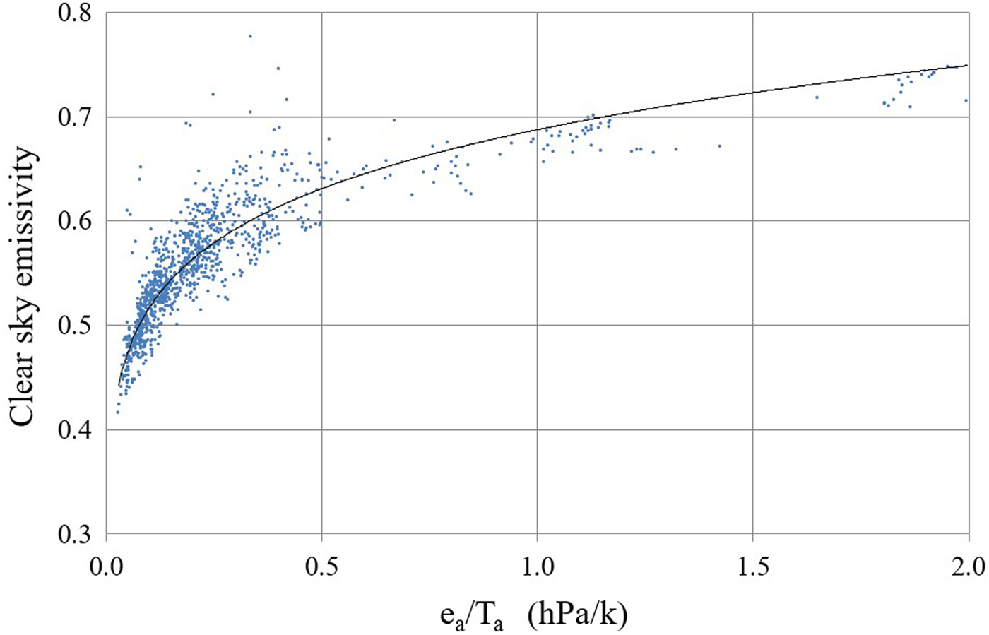
Fig. 2. Dependence of clear-sky emissivity on e a/T a at AWS3 for the cloudless dataset (n = 1455). Parameterization of Konzelmann and others (Reference Konzelmann, van de Wal, Greuell and Abe-Ouchi1994) is shown as a solid black line (p1 = 0.387; p2 = 8).

Fig. 3. Daily-average effective cloud-cover fraction N L (gray bars), with red lines showing 9-day running mean; blue line is 9-day running mean cloud transmission factor (trc). All three AWS sites are plotted for study period 2011/12.
4.4. Incoming shortwave radiation and N S
An annual mean of 63% of top-of-atmosphere shortwave radiation arrived at the glacier surface, with the remainder scattered by air, absorbed by gases and water vapor, attenuated by aerosols, reflected by cloud, and shaded by surrounding terrain. During summer, S ↓ was substantially greater owing to the higher solar zenith but was weakened by low transmissivity (Fig. 3) caused by cloud.
S ↓cs was calculated following the model of Bird and Hulstrom (Reference Bird and Hulstrom1981), at both 30 min and daily resolutions. The RMSE between modeled and observed radiation in the cloudless datasets at 30 min and daily resolution were respectively, 2% and 9% of the mean (mean = 687 W m−2, when data with shading by surrounding terrain were not included). The optimized model used an aerosol extinction coefficient (x) of 0.991, representing a low aerosol optical depth. trc was calculated using Eqn (5), and its daily average variation is plotted in Figure 3. Extended periods of high trc were seen from September to March, with generally lower values observed during summer.
By rearranging Eqn (10) for N trc = 1 and following Conway and others (Reference Conway, Cullen, Spronken-Smith and Fitzsimons2015), the relationship between k (1 − trc) and e a during overcast conditions were defined. A weak linear relationship between k and e a (R = 0.468, n = 84, P < 0.001) was found (Fig. 4), as shown by Eqn (11) below (N L,day > 0.8, the cloud fraction during daytime). The values of k are similar to those for Kersten Glacier (Mölg and others, Reference Mölg, Cullen and Kaser2009) and to the suggested value of 0.65 by Hastenrath (Reference Hastenrath1984).
 $$k = 0.0245e_{\rm a} + 0.6062{\rm \;} {\rm.} $$
Using Eqns (10) and (11), N S was derived for the three AWSs. The modeled N S values were slightly smaller than N L,day (Table 2). During summer, to further test the performance of derived cloud, correlations between N L,day and N S in the daytime were calculated (Table 4). The strong correlation between daily average N L,day and N S (0.78 < R 2 < 0.83) gave us confidence in the model results.
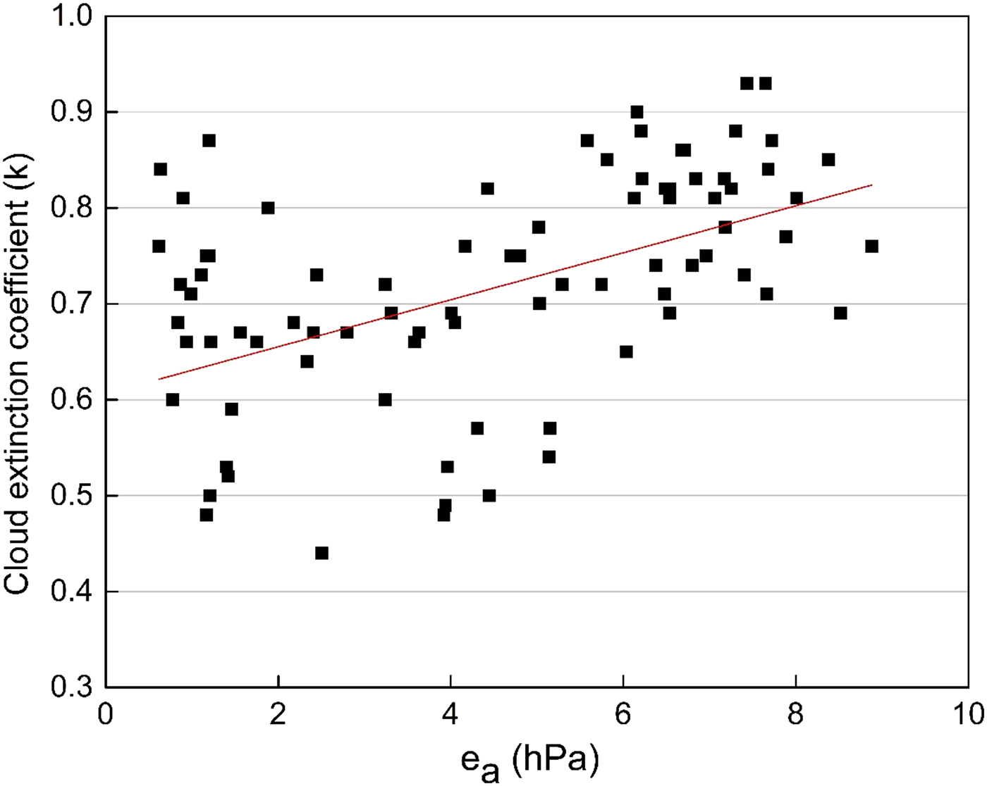
Fig. 4. Scatter plot of cloud extinction coefficient (k) and vapor pressure (e a) for overcast days (N L,day > 0.8).
Table 4. Correlation (R 2) between daily average cloud metrics derived at AWS1, AWS2 and AWS3 for period 1 January 2011–31 December 2012
To examine transferability of the cloud metrics to an on-glacier site, the correlation coefficients of daily average cloud metrics were calculated (Table 4). Strong correlations (R 2 ≥ 0.9) of N L between any two sites indicate the spatial consistency of cloud cover between sites and thereby validate the use of cloud data from one site to calculate S ↓ or L ↓ in a distributed glacier energy and mass-balance model (e.g., Arnold and others, Reference Arnold, Willis, Richards and Lawson1996; Brock and others, Reference Brock, Willis and Sharp2000; Hock and Homgren, Reference Hock and Homgren2005). The weakest correlations (0.6) were between N s at AWS1 and N L at AWS2, and between N s at AWS1 and N L at AWS3. This might be attributed to diurnal cycles in cloud cover or errors in measured data.
4.5. Seasonal variability in cloud
The 2-year AWS dataset covering 2011/12 was used to construct the preliminary climatology of cloudiness. Compared with N S, N L was more transferable and so its values were used to indicate monthly cloud variations (Fig. 5). There was a clear seasonal cycle in cloudiness. The majority of overcast days were in summer (May–August), accounting for 71% of the annual total. The largest fraction of overcast days was in July, reaching 27% at AWS2. In contrast with AWS1 and AWS2, the largest fraction of overcast days occurred in August at AWS3. The fraction of clear-sky days was slightly larger at AWS3 than AWS1 and AWS2. The largest fraction was in October and the smallest in July. From September to December, the climate was dry and cloudless and the fraction of overcast days was near zero at AWS3.
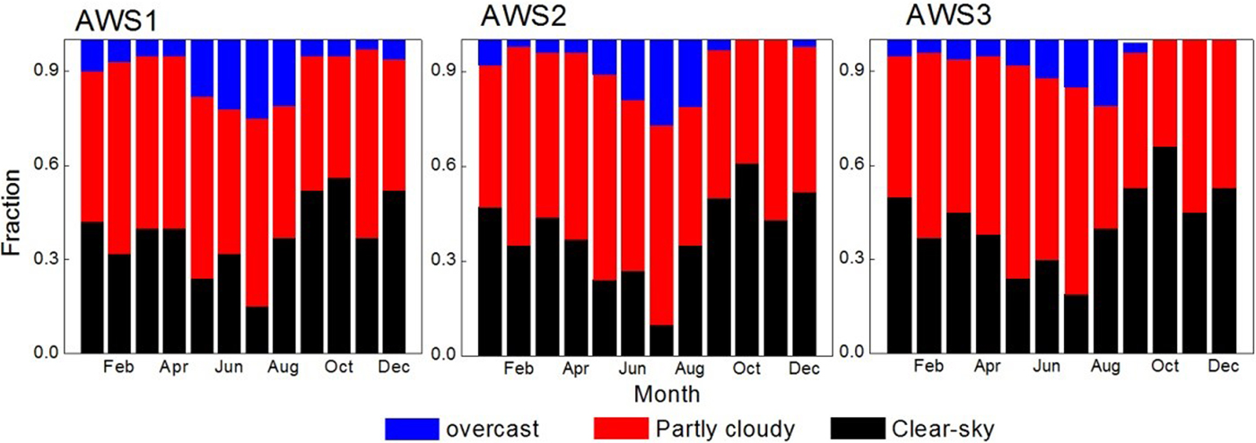
Fig. 5. Monthly fraction of clear-sky (N L < 0.2), partly cloudy (0.2 < N L < 0.8) and overcast (N L > 0.8) conditions at three AWS sites.
5. DISCUSSION
5.1. Cloud impacts on incoming shortwave and longwave radiation
Both S ↓ and L ↓ are influenced by air mass and cloud variability. We simply derived differences between observed actual and modeled clear-sky radiation to assess the influence of cloud on incoming radiation. Figure 6 shows a monthly mean change in S ↓ and L ↓ at the three AWS sites during 2011/12. In general, variability in both S ↓ and L ↓ was greatest in summer, owing to frequent cloud cover and the most striking change was in July 2012 at AWS3, with observations of −204 W m−2 for S ↓ and 71 W m−2 for L ↓. Annually, ~18% of top-of-atmosphere shortwave radiation was attenuated by the clear-sky atmosphere, 7% was shaded by the surrounding hills, while clouds attenuated a further 12%. The influence varied little with elevation. The annual mean change in S ↓ was 4 W m−2 greater at AWS2 and AWS3 than AWS1, and there was 5 W m−2 greater L ↓ at AWS3 than at AWS1 and AWS2. Mean annual and summer impacts were also determined (Table 5), clearly revealing that an increase in L ↓ could not offset a decrease in S ↓ either on a summer or annual timescale. There was a stronger gradient during the summer months. Conway and others (Reference Conway, Cullen, Spronken-Smith and Fitzsimons2015) found a more striking attenuation of shortwave radiation by the clear-sky atmosphere (23%) and by clouds (31%) at Brewster Glacier, because of its more humid atmosphere and more frequent clouds.

Fig. 6. Monthly mean influence of cloud on incoming shortwave (red line), longwave (blue line) and net radiation (black line) at three AWS sites during 2011/12.
Table 5. Annual and summer (May–September) mean reduction in S ↓ and Snet and increase in L ↓(W m−2) caused by cloud
Net radiation (Rnet) can be partitioned into net shortwave (Snet) and net longwave (Lnet) radiation fluxes. In many high altitudes and high latitude environments, variations in summer ablation are closely linked to change in Rnet (Sicart and others, Reference Sicart, Hock and Six2008). At Laohugou glacier No. 12, Rnet was the primary energy source in the surface energy balance (Sun and others, Reference Sun2012, Reference Sun2014). Although the increase in L ↓ could not offset the decrease in S ↓, the increase in L ↓ was always larger than the decrease in Snet (Table 5), except during summer at AWS2. Figure 6 shows the impacts of clouds on Rnet (black line) at AWS1 and AWS2. Owing to the high albedo at AWS1, Snet was less important and clouds always contributed to Rnet. The opposite pattern occurred at AWS2 during the melt season (May–September). Annually, Rnet was increased by 21 W m−2 under the impact of clouds at AWS1 and 2 W m−2 at AWS2.
5.2. Turbulent heat flux under different cloud conditions
Turbulent heat flux (Sensible heat flux (SE) and Latent heat flux (LE)) is important to glacier melt and studies have demonstrated that SE may contribute 7–23% and LE − 57% to 5% to glacier melt on TP glaciers (e.g., Kayastha and others, Reference Kayastha, Ohata and Ageta1999; Aizen and others, Reference Aizen, Aizen and Nikitin2002; Li and others, Reference Li, Liu, Zhang and Shangguan2011; Yang and others, Reference Yang2011; Sun and others, Reference Sun2012, Reference Sun2014; Zhang and others, Reference Zhang2013; Azam and others, Reference Azam2014). SE accounted for 28% of the surface energy source and LE accounted for 32% surface output at AWS1 during 1 June–30 September 2009 (Sun and others, Reference Sun2012). In the ablation zone (AWS2), the contributions were smaller than those at AWS1, and SE accounted for 7% of the surface energy output and LE for 15% during 1 June–30 September 2011 (Sun and others, Reference Sun2014).
Turbulent heat fluxes are related to near-surface gradients in temperature, water vapor pressure and wind speed (e.g., Oerlemans, Reference Oerlemans2000; Wagnon and others, Reference Wagnon, Sicart, Berthier and Chazarin2003; Mölg and Hardy, Reference Mölg and Hardy2004; van den Broeke and others, Reference van den Broeke, van As, Reijmer and van de Wal2004). Therefore, we analyzed monthly mean meteorological anomalies under various cloud conditions during May–September (Fig. 7). At AWS2, the cloud was always associated with a decrease in glacier surface temperature, except during August and September, and the temperature difference between clear-sky and overcast days reached 2°C in July. At AWS1, the temperature during overcast days always was higher than that of partly cloudy days, except during June, and the temperature of clear-sky days was higher during May, June and July. This may be explained by cloud cover reducing incoming solar radiation, which in turn lowers air temperature (Fig. 6). In August, most overcast and partly cloudy days were in the beginning and middle of the month, and clear-sky days at the end of the month. This was why air temperature on cloudy days was similar or higher than that on clear-sky days. Although the effect of clouds could increase surface air temperature in some months, cloudy periods usually occurred during days with weak melting.

Fig. 7. Meteorological factors (air temperature, vapor pressure and wind speed) plotted as monthly average anomalies of clear-sky (N L < 0.2), partly cloudy (0.2 < N L < 0.8) and overcast (N L > 0.8) days during May–September.
Water vapor pressure increased with cloud cover at AWS1 and AWS2 because of the greater moisture content associated with clouds. This relationship was weaker in July. Though the relative humidity was higher on cloudy days than on clear-sky days during summer, water vapor pressure could not exceed the saturated water vapor pressure at a certain temperature (Alduchov and Eskridge, Reference Alduchov and Eskridge1996). Cloudiness strongly reduced surface air temperature in July (Fig. 7), and low air temperature corresponded to a low saturated water vapor pressure. Such pressure on cloudy days might approximate water vapor pressure on clear-sky days with high air temperature. This could also explain why water vapor pressure increased most on cloudy days in August, because the air temperature on cloudy days was similar to or higher than that on clear-sky days.
With the appearance of clouds, air temperature declined, hindering the formation of katabatic winds. In general, wind speed was weakest during overcast days, most evidently during August and September. Sun and others (Reference Sun2014) quantified the sensitivity of mass balance to wind speed, finding that a wind speed variation of ±0.3 m s−1 could produce a ±26.9% variation of SE and ±1.5% variation of the LE, equivalent to 33.5 mm w.e. glacier melt or 2% of total melt during the observation period at AWS2. Wind speed during clear-sky days was always at least 0.3 m s−1 faster than that during overcast days at AWS2, except during May.
To further quantify the influence of cloud on turbulent heat fluxes, the SE and LE were calculated under different cloud conditions using the bulk aerodynamic method (e.g. Oke, Reference Oke1987), including the stability correction based on Monin–Obukhov similarity theory. A detailed description of the method is in Sun and others (2012 and 2014). Figure 8 shows the monthly average SE, LE and SE + LE under clear-sky, partly cloudy and overcast days. SE greatly decreased with the increase of cloud fraction at both AWS1 and at AWS2. Because of high water vapor pressure and weak wind speed, LE was weakest on overcast days and slightly stronger on clear-sky days than on partly cloudy days. At AWS1, the sum of SE and LE on clear-sky days was much larger than that on partly cloudy and overcast days, and slightly larger on partly cloudy days than on overcast days at AWS1 (except during May). At AWS2, the sum of SE and LE on clear-sky days was larger during warm months (May–July) and smaller than on overcast days during August and September. It was always larger on overcast days than on partly cloudy days.
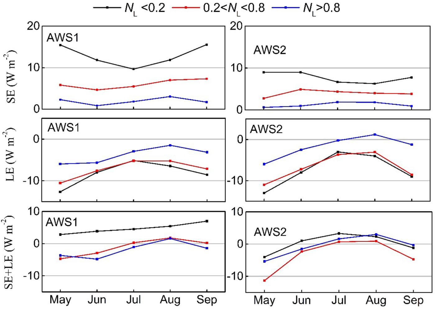
Fig. 8. Monthly average sensible heat flux (SE), latent heat flux (LE), and their sum under clear-sky (N L < 0.2), partly cloudy (0.2 < N L < 0.8) and overcast (N L > 0.8) days during May–September.
5.3. Melting during days with variable cloud cover
To assess the effect of cloud on glacier melt, accumulated mass balance was determined following the method in Section 3.2 for January 2011–December 2012 at AWS1 and AWS2 (Fig. 9). The total net mass balance was 320 and −2425 mm w.e. at AWS1 and AWS2, respectively. From October to March, there was small snow accumulation and very little melt. April–September was the main precipitation period (accounting for 86% of the annual total) and main melt period. Glacier melt was more intense in 2011 than in 2012, owing to a mean annual air temperature 0.7°C higher, and April–October precipitation was 50 mm w.e. less in 2011 than in 2012. Albedo was also lower during 2011, dropping to 0.38 at the end of the 2011 melt season at AWS1 and a negative net mass balance in 2011 indicated no net accumulation in the so-called accumulation zone (e.g. Wang, Reference Wang1981; Sun and others, Reference Sun2012).
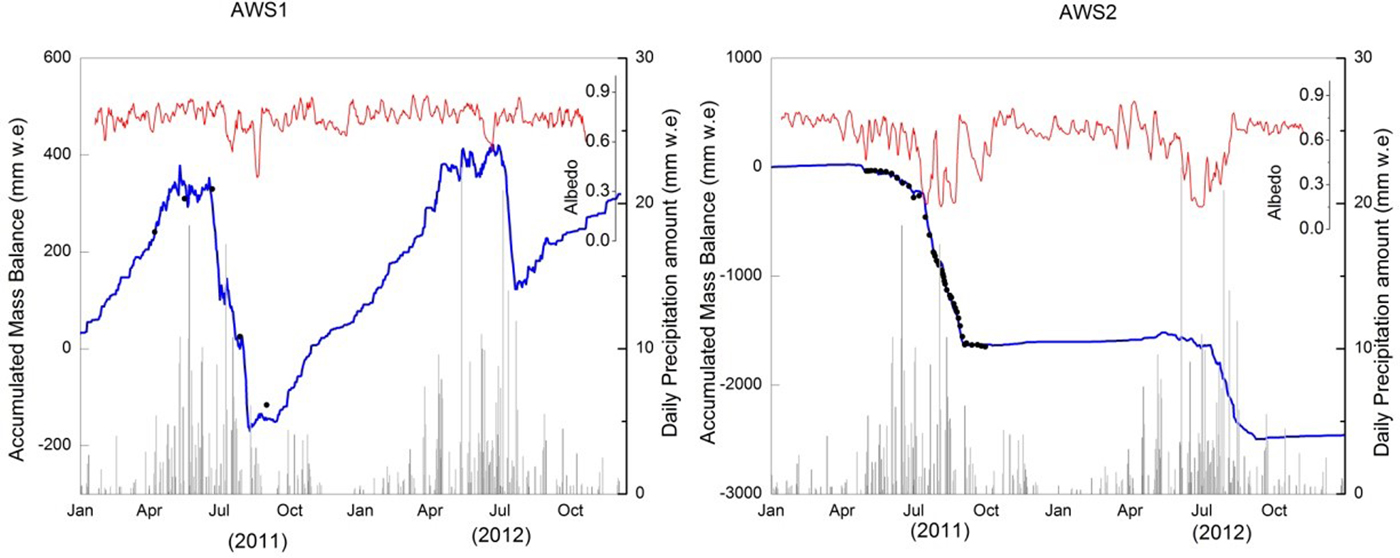
Fig. 9. Five-day running mean albedo (red line), daily total precipitation (gray bar), accumulated mass balance (blue line) and stake-measured mass balance (black dots) during 2011/12.
A dramatic loss of glacier accumulation area on many glaciers is an alarming problem. Two ice cores (from ~5800 m a.s.l.) retrieved at Mount Nyainqêntanglha and Mount Geladaindong on the southern and central TP provided evidence that the two coring sites had not received net ice accumulation since at least the 1950s and 1980s, respectively (Kang and others, Reference Kang2015). The problem of vanishing accumulation areas poses a threat to environmental information archived within the glacier ice layers (Zhang and others, Reference Zhang, Kang, Gabrielli, Loewen and Schwikowski2015).
The monthly mean daily net mass balance (not including snowfall days) during clear-sky, partly cloudy and overcast days are presented in Figure 10. The most intense melt was during July and August, with average melt reaching 7 mm d−1 at AWS1 and 24 mm d−1 at AWS2. Cloud suppression of glacier melt was very obvious at AWS2, especially in July, when melt was reduced by ~35 mm d−1 during overcast days compared with clear-sky days. There was a more complicated cloud effect on glacier melt at AWS1. Melt during overcast days was less than that on clear-sky and partly cloudy days. Melt on partly cloudy days during June, August and September exceeded that on clear-sky days but had comparable magnitudes. Melt during clear-sky days in May and July far exceeded that during partly cloudy days.
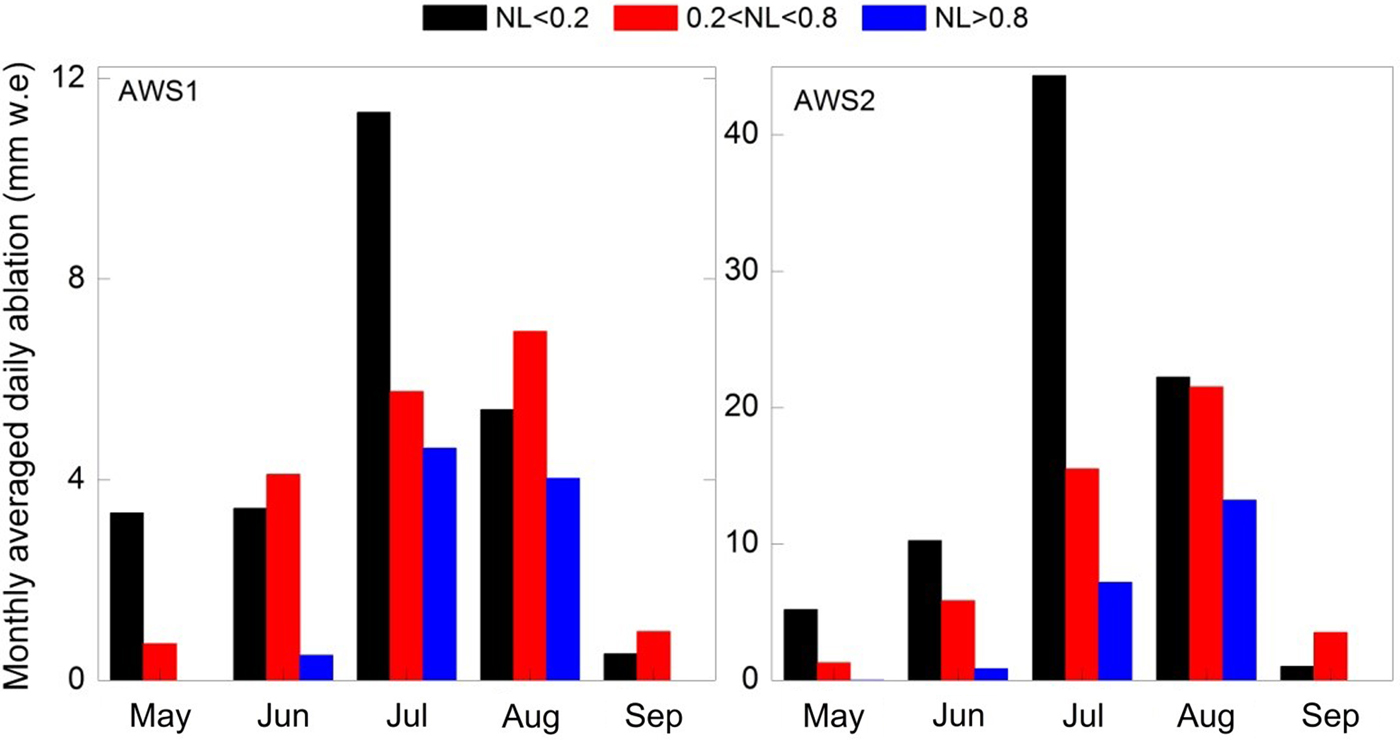
Fig. 10. Measured daily average net mass balance (mm w.e) of clear-sky (N L < 0.2), partly cloudy (0.2 < N L < 0.8) and overcast days (N L > 0.8) during summer (May–September).
In general, the appearance of cloud could protect glaciers from the intense melt. S ↓ is the primary source of energy in the surface energy balance of Laohugou glacier No. 12 (Sun and others, Reference Sun2012, Reference Sun2014), although in some months increases in Lnet exceeded decreases in Snet caused by clouds (Fig. 6). Nevertheless, most of the melt occurred in the daytime when S ↓ dominated Rnet. L ↓ followed no obvious diurnal cycle (Sun and others, Reference Sun2012), but the effect of cloud on S ↓ was largely during the daytime, so we infer that the increase in Lnet could not offset the decrease in Snet from cloud during the daytime. The reduced turbulent heat flux during cloudy periods further decreased melt on the glacier (Section 5.2).
On the Keqicar Baqi glacier southwest of the Tianshan Mountains, there is a strong negative correlation between relative humidity and Rnet during the ablation period (Li and others, Reference Li, Liu, Zhang and Shangguan2011). In view of the close connection between relative humidity and cloud fraction, and the great contribution of Rnet to the energy source on this glacier, we infer that cloud can reduce glacier melt. Jiskoot and Mueller (Reference Jiskoot and Mueller2012) found a substantial decrease of melt during overcast days compared with clear-sky days on Shackleton glacier in the Canadian Rockies. In fact, on these continental glaciers, Snet dominates melt and its decrease by cloud has strongly reduced melt (e.g., Aizen and others, Reference Aizen, Aizen and Nikitin2002; Li and others, Reference Li, Liu, Zhang and Shangguan2011; Zhang and others, Reference Zhang2013; Sun and others, Reference Sun2014). However, not all glaciers experience reduced melt during cloudy skies. In the ablation zone of Brewster Glacier, Conway and Cullen (Reference Conway and Cullen2016) found that during overcast conditions, positive Lnet and latent heat flux allowed melt to persist over a much greater period as compared with clear-sky conditions, leading to a similar amount of melt under each sky condition. Gillett and Cullen (Reference Gillett and Cullen2011) also found that the greatest melt events were associated with overcast conditions and contributed to proportionally larger changes in melt on Laohugou glacier No. 12. From the work of van den Broeke and others, (Reference van den Broeke, Smeets and van de Wal2011), we infer that melt rates are higher during overcast conditions at the lowest site of the Greenland ice sheet. In July 2012, a historically rare period of extended surface melt was observed across almost the entire Greenland ice sheet, which resulted from low-level clouds via their radiative effects (Bennartz and others, Reference Bennartz2013). The clouds brought more energy to that ice sheet via their radiative effects, but the ice sheet responded to this energy by reducing meltwater refreezing (Van Tricht and others, Reference Van Tricht2016). In the ablation zone of Parlung No. 4 glacier southeastern TP, Snet varied much less during summer. However, L ↓ showed a great difference because of the increase of cloud, which enhanced glacier melt (Yang and others, Reference Yang2011). Those glaciers are in maritime climates, where Snet is less important than in a continental high-elevation climate, and where warmer air masses are associated with cloudy skies. Owing to its important yet variable influence on glacier melt, cloud cover variation under increasing global temperatures may be important to future glacier melt.
6. CONCLUSIONS
We compared measurements made with three identical AWSs in the western Qilian Mountains during January 2011–December 2012. Two of the three were installed on Laohugou glacier No. 12 (5040 and 4550 m a.s.l.) and the third was in a meadow zone 1.6 km from the glacier terminus (4200 m a.s.l.). Except for wind speed and direction, daily mean values of all recorded variables exhibited synchronous fluctuations. Wind direction varied greatly between sites; westerlies dominated the wind direction in the upper glacier, while katabatic wind prevailed in its lower part.
In combination with clear-sky modeling, the variable effect of clouds on surface radiation fluxes was assessed. Derived cloud metrics from S ↓ and L ↓ were strongly correlated and of uniform magnitude. Owing to the effects of clouds and the atmosphere, top-of-atmosphere shortwave radiation was reduced by ~30% on average. The magnitude of the increase in Lnet caused by clouds exceeded the corresponding decrease in Snet over the glacier, except during July and August in the ablation zone.
Measured accumulated mass balances during the observation period were 32 mm w.e. at 5040 m a.s.l. and −2425 mm w.e. at 4550 m a.s.l.. May–September was the primary ablation period when the monthly mean daily accumulated ablation under different weather conditions revealed that melt weakened during cloudy conditions, particularly in the ablation zone. Analyses of air temperature, water vapor pressure and wind speed under various weather conditions indicated that increases in these variables tended to reduce energy reaching the surface, thereby reducing melt. Compared with glaciers in maritime climates, those in a continental climate are inclined to melt less under cloudy skies. However, this pattern may change as global temperatures rise and therefore needs further attention.
Acknowledgements
The work was supported by Chinese Academy of Sciences (KJZD-EW-G03-04) and National Natural Science Foundation of China (41721091, 41401074). Open Foundation of State Key Laboratory of Hydrology-Water Resources and Hydraulic Engineering(No.2017490711). We are very grateful to scientific editor H. Jiskoot, reviewer J. Conway and another anonymous reviewer for their constructive comments and thoughtful suggestions. Many thanks are also extended to colleagues working at Qilian Shan Station of Glaciology and Ecological Environment. We thank Steven Hunter, M.S, from Liwen Bianji, Edanz Group China (www.liwenbianji.cn/ac), for editing the English text of a draft of this manuscript.


 Open access