


Introduction
One of the prime goals of the Arctic Ice Dynamics Joint Experiment (AIDJEX) is an improved understanding of the drift of pack ice. To this end one urgently needs accurate field observations of the deformation οf different types of pack ice performed on a variety of time and space scales. To partially satisfy this need a series of detailed mesoscale strain measurements were made at approximately 3 h intervals over a 30 d period in the spring of 1972 in the Beaufort Sea. These measurements are particularly useful since in earlier studies of sea-ice deformation—as reviewed for example, in Hibler and others (973[b])—there have usually been large and random time intervals between observations, making the computation of accurate time series impossible. Also, and perhaps even more important, those studies included no detailed investigation of the non-linear variations in the ice velocity field that result from inhomogeneous spatial variations or fluctuations in the deformation of the ice.
Therefore, our analysis described in this paper was undertaken with three primary goals in mind: first, to provide a detailed time series of the least-squares strain-rate tensor and vorti-city (complete with “error bars” due to the non-linearity of the ice velocity field) over the 25 d period, Julian day 88–113, (28 March–22 April), 1972; second, to study the magnitude and nature of the non-linear velocity fluctuations; and third, to compare deformation measures from different scales to determine coherent modes of deformation in differently sized arrays as well as scaling effects. These results can then be compared with predictions from theoretical drift calculations and with data collected on the remote-sensing overflights. Besides providing insight into the nature of pack-ice dynamics, such comparisons and information on inhomogenities in the ice velocity field are helpful in designing future strain arrays.
Approach
As a framework in which to view our analysis, it is useful to think of the pack as a large number of irregular ice floes packed closely together, with the compactness varying with season. In the summer when the compactness is low, the individual ice floes can readily be identified and the pack looks like a two-dimensional granular medium. In the winter when the compactness is near unity, the individual floes can no longer be clearly identified and the ice is criss-crossed by a number of irregular leads. A typical example of the pack-ice structure in winter is given in Figure 1, where we show a schematic diagram of active leads and ridging zones in the mesoscale strain area for one instant of time.

Fig. 1. Schematic diagram of the mesoscale strain array together with an overlay of active leads and ridging zones. Leads and ridges were obtained from a 1500 m aerial photo-mosaic taken on 6 April 1972.
Using such a conceptual model of pack ice, we can view the velocity of any point in the pack as consisting of a continuum velocity component (varying over lengths commensurate with the scale of meteorological variations) plus a fluctuation component due to the discrete small-scale nature of the pack ice. Such a partition of the velocity field is similar to that which can be done for a fluid where the motion of each molecule has a continuum component plus a fluctuation component. In the case of the pack ice, however, the fluctuations are probably not due so much to random motion of floes (although this is undoubtedly a factor) as to the fact that the floe sizes are large relative to our measurement scale and thus spatial velocity profiles will be of a stepped nature. This is illustrated by Figure 1, where, we see that the distance between leads, where relative motion occurs, is generally 4 to 6 km. Also, for pack ice, the fluctuations would be expected to be highly variable in time since they will primarily be driven by the transfer of energy into the pack by meteorological forces. This is different from the case of a fluid in a laboratory, where fluctuations are well described by the temperature.
As we examine spatial variations in the velocity field over larger and larger areas, the contributions of fluctuations to average velocity differences (i.e. strain-rates) would be expected to become less pronounced. Stated differently, one would expect the contribution of fluctuations to the sea-ice strain-rate to become small when the area covered by the strain array becomes large relative to floe size and/or distances between leads.
In order to sort out the fluctuations from the continuum motion we have analyzed the position data of the mesoscale targets by fitting a least-squares planar surface to the spatial velocity field sampled by the array, with the slope angles of the plane representing the strain-rate and vorticity. Such a procedure is commensurate with the discussion of sea-ice strain by Reference NyeNye (1973) where he notes that for a precise measure of the strain-rate one needs to first smooth the velocity field before taking derivatives. Since the area covered by the mesoscale array is relatively small (≈ 20 km diameter) compared to meteorological systems, we would expect the continuum velocity to be relatively linear over this region and hence the planar approximation should be good. Residual deviations from this planar surface are identified as fluctuations. These residual deviations will also cause some uncertainty in the strain-rates, an uncertainty which can be estimated by dimensional analysis for differently sized arrays on the assumption that the fluctuation amplitude is reasonably similar over the region. As part of this procedure to distinguish between continuum motion and fluctuations, we also estimate a continuum length which we define as the length over which, on the average, the continuum velocity differences equal the fluctuation amplitude. This length, which turns out to be about 10 km, gives us a rough measure of the scale above which sea ice may be viewed as a continuum and below which the discrete nature of the pack begins to dominate the motion.
Finally, in addition to such a least-squares analysis to look at scaling effects, we also compare strains obtained from triangles of different sizes (5 km to 20 km) and compare the mesoscale strain results over the 20 km region lo the macroscale strain results measured from a 100 km triangle, one corner of which is the center of the mesoscale array. The comparison generally indicates that all arrays are measuring similar continuum motions of the pack with the fluctuations yielding a large contribution, but not masking the continuum motion on a scale of about 20 km.
Site location and Data Collection Procedures
The measurements used for this study were made in the vicinity of the main 1972 AIDJEX camp, located at roughly lat. 75° 00’ N., long. 148° 30’ W. The camp as well as the different research programs carried out from it are described in AIDJEX Bulletin, No. 14, 1972. The strain array was established by erecting a series of targets which consisted of corner cubes mounted on the tops of aluminum poles. The distances to and angles between the targets were measured using a continuous-wave laser range-finder at two to three hour intervals. The height of the targets varied from 3 to 10 m above the ice surface depending on the distance and the obstructions between the target and the main camp. A diagram of the strain array is shown in Figure 1, together with an overlay of active leads and ridging zones. The angles to the targets were measured with an average accuracy of better than ± 1 min and were referenced to a fixed stake on the multi-year floe on which the main camp was sited. The line between the laser and the stake was then tied into the true north determinations (sun shots) made by Thorndike and Gill (Reference Thorndike, Thorndike, Martin, Bell, Virsnieks and GillThorndike and others, 1972). Distances were measured to the nearest 0.1 ft (0.03 m) because the large strains that were experienced obviated the need for any greater precision.
This strain measurement system was found to be vastly superior to the use of manned tellurometer sites (Reference Hibler, Hibler, Weeks, Ackley, Kovaes and CampbellHibler and others, 1973[b]). With it, a large number of strain lines could be determined easily without manning the remote stations. It was also relatively quick and easy to install and placed a minimal reliance upon “black boxes”. However, visibility problems (wind-blown snow, sea smoke from leads) made acquisition οf continuous, equally-spaced time series difficult (laser measurements were impossible approximately 10% of the time, and once high winds caused a gap of almost two days in the time series for the strain line) In addition, the system required manpower 24 hours a day.
Data Analysis
Extrapolation and smoothing of strain data
Data taken in the field consisted of distances and angles of targets relative to a fixed reference stake. As a first step in the data reduction, these angles were converted to angles relative to true north as measured on Julian day 81 (21 March). Rotations of the array were not taken into account for strain calculations, so that the coordinate system used for this study is slightly different from the true north coordinate system (the maximum difference is, however, less than 5 deg). Rotations of the array were, of course, included in the vorticity calculations. The time scale was converted to G.M.T. by using four G.M.T. calibration times obtained in the field to find a least-squares rate for the clock used in the measurements. The data point times were recomputed with this rate and then all data (both angles and distances) were linearly interpolated and resampled every hour. Using this new data set at one-hour intervals, the time series was smoothed with a low-pass filter having a transition band width with periods from 8.0 to 6.15 h. The smoothed time series was then resampled every third hour. If there was reason to expect that the data contained a large number of time intervals greater than 3 h, a low-pass filter having a transition band from 20 to 11.4 h was used before resampling. Both filters had less than 0.16% side-lobe errors and consisted of 81 symmetric weights designed according to the procedure discussed by Reference HiblerHibler (1972).
This process of interpolation followed by smoothing may be viewed as a consistent way of constructing a smooth curve (with no high-frequency components past a reasonable cut-off dictated by the average sampling rate) through the randomly spaced data points. Alternatively the curve may be considered an accurate representation of the low-frequency portion of the linearly interpolated curve.
Examples of the smooth curves generated by this process are shown in Figure 2, Curve a, which results from the filter with the higher frequency cut-off, follows the data quite closely. This indicates that there is little variance associated with periods shorter than 6 h.

Fig. 2. Typical restais of the interpolation and smoothing process used to generate equi-spaced values for Ike strain analysis. Curve a was obtained with a smoothing filter transition band from 8.0 to 6.15 h and curve b with a transition band from 20.0 to 11.4 h.
Experimental error estimation
The primary source of error in the measurements is the uncertainty of target angles. Since angular measurements were generally accurate to ±0.000 3 rad (± 1 min) and distance errors were small, we estimated the x and y position errors of each measurement of a target at distance r and angle θ to be

Since measurements three hours apart were subtracted to obtain velocities we estimated x and y velocity errors to be

with Δt = 3 h. This is a slight over-estimation of errors for the difference between two numbers with uncorrelated errors. However, since there may be some errors due to interpolation between inequally spaced points that are not removed by smoothing, we have made a conservative error estimation. The experimental errors given by Equation (2) were then used as input to obtain the experimental error on the strain-rate tensor as discussed in the next section.
Least-squares computational technique
To understand conceptually the least-squares strain and vorticity calculations, it is useful to visualize a contour plot of the x (ory) velocity component of the ice. In essence the computer program used to calculate the deformation rate fits a planar surface through the contour plot with the slope angles of the planes yielding the strain-rates and voriicities. Since the actual velocity components will deviate from a perfect plane, there will be some uncertainty in the slope angles of the plane. We refer to the average deviation οf the velocity components from the plane as the residual fluctuation error and the uncertainty in the slope angles of the plane is referred to as the inhomogeneity variation. In addition, once the least-squares equation for the plane as a function of say N velocity measurements is determined, the estimated experimental errors may be inserted to obtain estimates of slope uncertainties due only to experimental errors. The remainder of the slope uncertainty may then be identified with non-linearities in the ice velocity field.
To formulate this conceptual model mathematically we proceed as follows. Using tensor notation for the strain-rate, the strain-rate tensor ė and vorticity ϖ are defined by

where vi is the ith velocity component of the ice pack (considered as a continuum) and i, j = 1, 2 since we are only concerned with the horizontal motion of the sea ice. Considering N targets whose positions are being measured, we denote by  the measured jth velocity component of the ith target, and by θi and ri the polar co-ordinates of the ith target relative to an arbitrary origin.
As a model to explain the velocities of the N targets, we consider the ice velocity field (on the scale of about 20 km) to consist of a continuum velocity component, which varies in a uniform linear manner, (specified by  and ϖ) plus a random fluctuation component. Mathematically our model is expressed by the equation

where

and A 1, A 2 are constants representing the continuum velocity components at the origin. In Equation (3), zi is the fluctuation component plus any measurement error and E(ui) = xij εj is the “expected” value of ui since E(zi) = 0. The least-squares estimates of єi, denoted by ê i, are obtained by minimizing ∑ zi 2.
To do this we differentiate

with respect to εk which yields the matrix equation for the least-squares estimates of εi (Reference Jenkins and WattsJenkins and Watts, 1968, p. 132):

where M = X TX and T denotes transpose.
When using these least-squares equations, it should be noted that adding a constant rotation to all angles only changes the vorticity ϖ. This can be demonstrated by noting that in Equation (3) changing ϖ to  changes ui to ui’ where

This, however, is equivalent to adding a constant rotation per unit time to all angles. In a similar manner, adding a constant velocity to all points changes only A 1, and A 2
Since we have only a finite number of random velocity measurements (each with some random fluctuation “error”) with which to calculate  there will be some uncertainty or error in . TO estimate this variation or uncertainty it is necessary to calculate the covariance matrix of which is easily shown (Jenkins and Watts, 1968, p. 134) to be given by

where  and Vij = cov (zi, zj). In our case zi consists of two parts

where zi M is the measurement error (which we estimate to be given by Equation (2)) and zi I is the fluctuation component of the ice motion due to the fact that the actual ice velocity field is non-linear. If we assume that zi M and zi I are uncorrelated, then the variation in ê i due only to measurement errors, call it Cij M, may be estimated using Equation (6) with Vij M = cov (zi M, zi M). Using Equation (2) we estimate Vij M to be

To find the variation of some linear combination of the due to the total “error” zi, we make the usual assumption that the zi are uncorrelated with the same mean and variance so that cov (zi, zj) = δij σ 2 where the point estimator of σ 2 (denoted by s 2) is given by the residual error

where  .
.
In this case Equation (6) reduces to

Given a linear combination of  then the deviation of
  from
from  is such that

has the t distribution with 2N—6 degrees of freedom, assuming that the errors are normally distributed (Reference Bennett and FranklinBennett and Franklin, 1954, p. 250). Consequently, confidence limits for the estimated strain may be obtained using a t-distribution table.
In addition to the estimated strain, we are also concerned with the velocity fluctuation component zi I which is strictly speaking not an error, but represents the variation from linearity of the velocity field over the region sampled. In the cases we have studied, the estimated residual error zi obtained from Equation (8) was generally found to be larger than the average estimated value of experimental error zi M from Equation (2). Consequently as a matter of convenience, we will often refer to the residual error obtained from Equation (8) as the residual fluctuation error.
Also, as a matter of notation we will refer to the uncertainty in  , as the inhomogeneity error. It should be remembered that the inhomogeneity error is an estimate of the uncertainty in the least-squares estimated strain and consequently will depend some-what on the number of samples used. The residual fluctuation error, on the other hand, should be relatively independent of the number of sample points used.
Strain Results
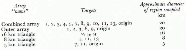
For comparison, time series of the strain-rate and vorticity have been calculated using several different combinations of targets; Table I describes all combinations of targets used in the calculations. The origin was also considered a position measurement in some arrays, with distance and angle being zero for all time.
Table I Strain-Line Combinations Used in this Paper.
Over the time interval studied in this paper, there was only one major gap in the time series, and this portion is blanked out in the plots. However, for spectral studies, root-mean-square error estimation, and correlation studies, the whole curve was used (data points every 3 h) including linearly extrapolated data through the gap, with the linear extrapolation being done on each target position as discussed previously.
Time series of the strain tensor
Since the outer array targets were measured more often than other targets, the outer array provides a more detailed time series for analysis. Results of least-squares calculations using the outer array are shown in Figures 3 and 4 which present the two invariants (Reference NyeNye, 1957) (denoted by  and
and  ) of the strain-rate tensor both separately and in the form of the divergence rate
  (sum of the principal components) and the maximum shear rate
  (half the difference of the principal components). For the strain-rates, the angles of the strain lines at the beginning of each 3 h interval were used in the least-squares calculations. The continuous errors in Figures 3 and 4, which are the ∆ values shown below each curve, represent the inhomogeneity error (calculated using Equations (8) and (9)) which is due primarily to velocity fluctuations. The small error bar on the divergence-rate curve represents the maximum experimental error, which was calculated by first calculating the experimental
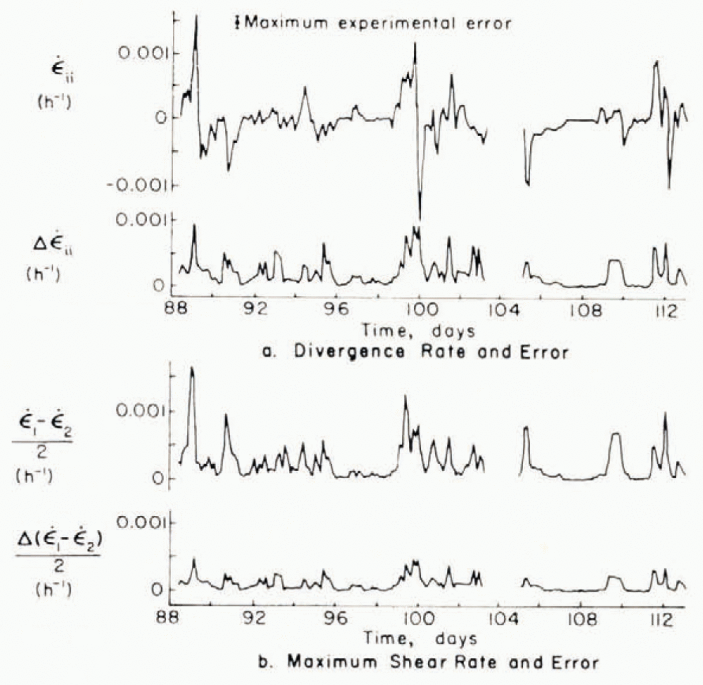
Fig. 3. (a)Least-squares divergence rate and accompanying inhomogeneity error and (b)maximum shear rate and inhomogeneity error. The small error bar in (a)represents the maximum uncertainty due to measurement error.
Fig. 4. (a)Principal axis components of the least squares strain-rate tensor and (b)inhomogeneity errors.
error for each point in the time series according to Equations (6) and (7) and then finding the maximum error over the time series. For a more compact summary of the relative magnitude of the strain-rates and strain-rate variation errors we list the r.m.s. values for the various time series in Table II.
Table II Table II. R.M.S. Strain-Rates, Strain-Rate Variation Errors and Experimental Errors for Outer Array.

It is clear from the figure and from Table II that in general strain-rates are of greater magnitude than their respective strain-rate inhomogeneity errors. The figures also indicate that the inhomogeneity error generally increases with increasing strain-rate. It is important to remember that the inhomogeneity errors shown are for six targets and would be smaller for a larger number of targets. This is analogous to the error on the slope of a simple least-square line, which becomes less as more points are added even though the standard error of the estimate may remain the same. In particular, for the same residual error for each velocity, an equilateral strain triangle would have a divergence-rate error c. 1.7 times as large as that shown in Figures 3 and 4.
One striking aspect of the deformation, best illustrated in Figure 4 is that in the principal-axis coordinate system most of the expansion or contraction is taking place along one axis. Moreover, there is usually contraction along one axis and extension along another. Another salient characteristic of the ice deformation is that the ice motion appears to consist of deformational events which occur every several days and usually consist of dilation followed by convergence.
The time series of the strain-rate generally shows rather rapid variations in strain which are probably due to the random bumping and yielding of floes as well as the random opening of leads. Under our idealized model consisting of ice fluctuations superimposed upon a continuum, these high-frequency motions should primarily represent fluctuations. The maximum observed divergence rate is seen to be (0.16% ±0.09%) per hour and the maximum convergence rate (0.15% ± 0.09%) per hour. The largest maximum shear rate is (o.16% ± 0.09%) per hour.
Non-linear velocity fluctuations
The least-squares calculation, besides yielding the average strain-rates, also give a measure of the non-linearity in the velocity field through the residual fluctuation error. This residual error can be viewed as a fluctuation in the velocity field from the ideal continuum value. The magnitude of these fluctuations is important for determining the size of a measurement array necessary for accurately measuring the average strain-rate. In terms of our continuum model, the fluctuation contribution together with the average strain-rate yields a characteristic length above which the pack ice may be considered a continuum and below which the ice motion of individual floes and leads becomes dominant. Such a characteristic length is estimated by determining on the average the length over which the fluctuation is almost the same as the continuum velocity variations.
For a best estimation of the fluctuation error we utilized the combined array consisting of 11 targets plus the. origin. Since some targets in the combined array were not measured as frequently as those in the outer array, the linearly extrapolated data were smoothed with a filter having a transition band from 20.0 to 11.4 h as discussed in the previous section on data analysis.
The resulting residual errors from the combined array and strain tensor components in a (north, west) co-ordinate system are shown in Figure 5. In order to put the residual error and deformation rates in perspective to the overall motion of the pack ice, we have also shown, in Figure 5, plots of the velocity components of the central point of the array. These velocity plots were obtained using drift data obtained by Thorndike and others (1972) from satellite navigation fixes. We have smoothed the velocity data with the same filter used in the strain calculation. In the processing of the data carried out by Thorndike, some smoothing was also carried out, but this smoothing only affected the higher frequencies past the transition

Fig. 5. Comparison of (a)mesoscale divergence rate, (b) north–south strain-rate, (


band of our filter. For a more concise comparison of the data, r.m.s. values of the various curves are given in Table III.
Table III Strain-Hates, Residual Errors, and Central-Point Velocities (from Fig. 5).

As can be seen from Table III, the characteristic length (residual error/strain-rate) over which the velocity change due to strain-rate is of the same magnitude as the residual fluctuation error is of the order of 10 km. A second characteristic length of some interest is the length over which the velocity difference according to the strain-rate equals the average drift velocity. This length is seen to be about 1 000 km, roughly similar to the size of the Pacific Gyre. Consequently we see that the residual error is rather insignificant in terms of the absolute velocity for a point but becomes more critical in terms of the velocity gradient or deformation rate. In terms of a continuum model the results suggest that on a scale larger than about 10 km the pack ice begins to behave like a continuum, whereas on a smaller scale the individual particle behavior begins to dominate the observed motion.
The magnitude of the residual error also allows us to estimate the effect of fluctuations on strain-rates from arrays of different sizes. For example, we can view the strain measured by a simple area, say a triangle, to consist of two components: (1) the continuum strain-rate and (2) the fluctuation component. Assuming that the residual error is approximately constant, independent of the size of the triangle, then the fluctuation contribution to the strain-rate will be of greater relative magnitude for small triangles. In addition, since the fluctuation component would be expected to consist of rather rapid bumping motions, strain-rates would behave in a more erratic manner as the measuring triangle becomes smaller. This effect is apparent in plots of individual triangles. In Figure 6, for example, we illustrate the net divergences (essentially the areas) of three nested triangles as a function of time. The more rapid, large-magnitude motion of the small triangles is apparent. The curves do, however, illustrate a general correlation of strain events consisting of dilation followed by convergence. Generally these results suggest that although the smaller triangles are averaging over very few leads and/or floes, over a period of several days the ice on a small scale would be expected to diverge if the pack is generally diverging and converge if the pack is converging.
Comparison of Mesoscale Deformation to Macroscale Deformation
In addition to a satellite navigation system at the main 1972 AIDJEX camp (the center point of the mesoscale array), the 1972 pilot study included satellite position measurements of two other camps approximately 100 km west and north-west respectively of the main camp. Strain data from this larger triangle, which we refer to as macroscale deformation, provides a valuable measure of the deformation averaged over a larger region than that covered by the mesoscale array.
In a comparison between the macroscale and mesoscale deformation rates, arguments both for similarities and differences can be made. First, since weather systems typically vary over several hundred kilometers, one would intuitively expect some similarity between the macroscale and mesoscale deformation rates, at least to the extent that both systems are measuring the continuum motion of the ice pack. However, there are several reasons why the correlation should not be extremely good. Foremost is the fact that the mesoscale array is only slightly larger than the estimated continuum length of 10 km and thus fluctuations of the

Fig. 6. Comparison of net divergences (areas)of overlapping Mangles, (a)16km triangle, (b)8 km triangle, (c)5 km triangle.
velocity field yield a strong component in the time series of the least-squares mesoscale deformation, much stronger than would be expected to be present in the macroscale data. Also, even if the pack ice could be considered a homogeneous continuum at very small scales, the nature of the continuum constitutive law might couple with variations in the weather systems to give rapid variations in the deformation. This is especially true since the mesoscale array is not at the center of the macroscale array, but at one corner.
In order to examine differences and similarities between the macroscale and mesoscale deformation, and thus test some of the above hypotheses, a comparison both of the various deformation time series and their spectra was made. The macroscale deformation data were supplied by Allan Thorndike and are essentially the same data as presented by Reference ThorndikeThorndike (1974).
In the processing of the macroscale data, Thorndike employed a Kalman filtering procedure to obtain the position and velocity of each of the three satellite sites. The filter cut-offs varied somewhat but generally all frequencies up to a period of 18 h were passed. The strain-rates and vorticity were uniquely determined since there were only three stations.
Time-series comparison
In order that both time series be smoothed in the same manner, all deformation rates were smoothed with a low-pass filter with a transition band from 21 to 84 h. This smoothing also allowed a time series for the mesoscale vorticity to be constructed by adding in the camp rotation, a step that is difficult without extensive smoothing because azimuthal measurements were typically made only once a day. To obtain the camp rotation for the mesoscale calculation, a time series R = (sin ϕ) (longitude —azimuth) (with longitude increasing in an easterly direction, see Reference NyeNye (1974)) where ϕ is the latitude, was constructed by linearly extrapolating the satellite position and azimuth measurements reported by Thorndike and others (1972). This time series was smoothed by the same filter that was applied to the deformation data. This rotation rate was added to the vorticity calculation in the camp coordinate system to obtain the true vorticity as discussed in a previous section. For mesoscale data in the camp coordinate system, the least-squares results for the outer array were used. In addition, several days of earlier data (taken before the array was complete) consisting of only four targets (1, 2, 3, 8) plus the center point were used to extend the time series.

Fig. 7. Comparison of (a)mesoscale and macroscale divergence rates, (b)vorticities, and (c)maximum shear rates. The dashed lines represent macroscale data and the solid lines mesoscale data.
In Figure 7 we show a meso–macro comparison of the divergence rates, vorticities and maximum shear rates. The dashed lines represent the macroscale data. Due to a malfunction of one of the satellite navigation units, there is a gap of several days in the macroscale data which was bridged by Thorndike using a Kalman filter. This gap is indicated in Figure 7. For a quantitative comparison of the curves we give in Table IV correlation coefficients and r.m.s. values for the various curves up to the gap in the macroscale data. The standard error for the correlation coefficients is based upon a number of degrees of freedom equal to the number of points correlated times the fraction of the spectrum passed by the filter.
Table IV Mesoscale and Macroscale R.M.S. Deformation Rates and Correlation Coefficients (from Fig. 7).

Figure 7 and Table IV indicate that there are significant correlations between the time series for deformation measured at different scales. Visual examination of the curves suggests that the correlation is due to the presence of similar strain events over periods of several days, Since these events are often of different amplitude and occur at slightly different times, the correlation is not complete, especially at higher temporal frequencies. The results also show the deformation rates to have comparable amplitudes, with the mesoscale amplitude generally being slightly larger. The comparison generally indicates that both mesoscale and macroscale arrays are measuring similar continuum motions of the ice pack.
Spectral densities
Some of the important differences between the nature of the mesoscale and macroscale deformations are illustrated by the spectral densities which we calculated using the lag product method as discussed, for example, by Reference RaynerRayner (1971, p. 94). In Figure 8a we show the spectra of the mesoscale divergence rate and shear (not maximum shear) and in Figure 8b the spectra of the macroscale divergence rate, shear and vorticity. Because of the inadequacy of the lime series for the camp rotation at higher frequencies, it is not possible to construct a mesoscale vorticity spectrum. Also, because of the Kalman filter smoothing of the macroscale data, the macroscale spectra are valid only up to frequencies with about 15 h periods. Since there were differing data gaps, the spectra do not come from the same time periods, but were calculated from day 88 to 113 for the mesoscale data and from day 81 to 101 for the macroscale data.
From Figure 8 we see that the macroscale spectra generally contain less variance at higher frequencies than the mesoscale spectra. Such a result is commensurate with viewing the deformation as a continuum signal plus a fluctuation component with the fluctuation magnitude dropping off inversely with the size of the array. This follows because the fluctuation signal, being of a random nature, would be expected to have a greater high-frequency variance.
An interesting aspect of the mesoscale spectra (especially the divergence rate) is the presence of a significant spectral peak at about 12 h periods. Whether such a peak is contained in the macroscale data cannot be ascertained because the smoothing employed by Thorndike effectively filtered out any such oscillation. A possible explanation for this peak is a variation in water currents due to inertial oscillations Reference Hunkins(Hunkins, 1967). Measurements of ocean currents by Newton and Coachman Reference Newton and Coachman(1973) during previous AIDJEX pilot studies have indicated 12 h cycles in the currents with the oscillation displaying coherence over distances up to 20 km. Different drag coefficients for different ice floes could couple with

Fig. 8. Power spectra of (a) mesoscale divergence rate and shear rate, (b) macroscale divergence rate, shear rate and vorticity.
these currents to create a differential ice motion. There is also evidence of an approximately 24 h cycle in the macroscale divergence rate spectrum (which may possibly be present in the mesoscale data). The source of this peak is not at present understood.
The general fall-off of the spectra in Figure 8 is also relevant for sampling considerations. The shape of the spectra generally suggests that sampling intervals up to 10 h (with accurate measurements) would yield low-frequency information without intolerable aliasing. A more direct test of this can be made by sampling the data at larger intervals before smoothing and comparing this to data smoothed before resampling. Such comparisons have been made for the mesoscale data Reference Hibler, Hibler, Weeks, Kovaes and Ackley(Hibler and others, 1973[a]) and support the conclusion that accurate samples every eight hours are adequate for resolving the low-frequency components of the time series required for comparison with synoptic meteorological variations which generally occur over a time scale of several days Reference Monin(Monin, 1972).
Nature of the Ice-Pack Rotation
Examination of the mesoscale vorticity indicates that it is similar to the camp rotation. This can be seen from Figure 9 where we show the camp rotation rate and the mesoscale vorticity. This similarity means that to a large degree the whole mesoscale region is rotating as an entity. Investigation of the macroscale deformation data indicates that such a “solid” rotation is also partially occurring for the larger macroscale region, at least at low temporal frequencies. This may be seen from Figure 10 when the cast–west shear ∂vy /∂x and vorticity are plotted together. As can be seen, the two curves are similar, indicating that ∂vx /∂y and ∂vy /∂x are close to being equal in magnitude and opposite in sign, a condition which holds identically for solid rotation. Another indication of this behavior on the macroscale is the relative smallness at low frequencies of the macroscale shear-rate spectral density in the x–y co-ordinate system compared to the macroscale vorticity spectral density as shown in Figure 8b.

Fig. 9. Camp rotation rate and mesoscale vorticity.
These observations suggest that the most pronounced mode of differential deformation of the ice pack is a relatively cohesive rotation of the pack, at least at low frequencies. The direction of the rotation is, from the curves in Figure 10, generally clockwise in agreement with the motion of the Pacific Gyre. Other deformation rates at low frequencies appear to be somewhat smaller than the rotation rate. Such a cohesive rotation is also borne out by deformation studies in the shear zone (Reference Crowder, Crowder, McKim, Ackley, Hibler, Anderson, Santelbrd and SmithCrowder and others, 1974; Hibler and others, in press) suggesting that the pack is rotating as a relatively tightly bound continuum with slippage at the boundaries.
A final point of interest is a negative correlation between the vorticity and the divergence rate (see Fig. 7). The correlation coefficient for the mcsoscale data (omitting the earlier data taken before the mesoscale array was complete) is in fact —0.35 ± 0.17, indicating that a convergence is associated with a counter-clockwise rotation. This correlation is discussed in greater detail in relation to linear drift theories and atmospheric pressure variations in another paper (Reference HiblerHibler, 1974).

Fig. 10. Fig. 10. Comparison of east–west shear rate (∂vy /∂x)and vorticity for (a)mesoscale array, (b)macroscale array,
Conclusions
We believe that this study has shown that strains measured on a scale of to km or greater can serve as a valid measure of the continuum motion of sea ice. When strains are measured on a smaller scale, the continuum motion is obscurred by the random bumping and yielding of floes and by the finite size of the interacting floes relative to the size of the strain array. These small-scale motions are, of course, interesting in their own right. Our results also indicate that meaningful vorticity values can be obtained from even smaller arrays, indeed from the measured rotation of individual stations.
These results suggest that it should be possible to carry out highly useful experiments on the macroscale (continuum) behavior of pack ice by utilizing one manned drifting station or ship with radar transponders located at the remote strain points. Strain arrays with effective diameters of up to 50 km should easily be possible using currently available techniques.
Finally, it should be emphasized that our results were obtained from a pack-ice field with a compactness of near one and a specific, but unknown, ice thickness distribution. Whether similar results would be obtained for other conditions, is presently a moot point.
Acknowledgements
We would like to thank Dr W. J. Campbell for interesting us in developing a mesoscale strain program and for his valuable assistance during the field study. Thanks are also due to J. Taylor and G. F. N. Cox for their assistance with the manning of the laser array. Allan Thorndike kindly provided us with processed macroscale drift and deformation data and, together with A. Gill, provided us with information on the rotation of the base camp.
We would also like to thank Dr J. F. Nye for his comments on a draft version of the paper and A. Johnson for editing the final version. Finally we would like to thank the staff of the AIDJEX project for their support which made this program possible. This research was funded by the National Science Foundation under NSF Grants AG-344 and AG-492, and by ARPA under ARPA order 1615.


