Introduction

The flow of ice sheets and their interaction with climatic conditions involves the response of polycrystalline ice to stress and temperature over timescales of hundreds to thousands of years, which cannot be observed in laboratory experiments. However, ice-core data yield a variety of measurements of ice properties at the different depths down the core, including the corresponding ages of each ice element, which reflect the above timescales. These, though, are the ‘present’ states of the ice elements, which have evolved from some initial state as the ice element moves down the core from the surface. The correlation of the present statewith laws describing, for example, grain growth requires the motion history of each ice element: its particle path and deformation evolution. These, in turn, require the histories of the accumulation and strain rate.

We will make the conventional assumptions of purely vertical particle velocity and uniform compressive axial strain rate in the core, which yield a tractable one-dimensional analysis. The present surface accumulation is measured. To determine the past thickness, it is necessary to prescribe the history of melting (or refreezing) at the bed and to extend the above axial motion assumptions below the core, down to the bed, which is assumed here for illustration. To determine the surface- and bed-elevation histories it is then necessary to prescribe an additional bed condition (e.g. a rigid-bed assumption), but conditions below the core do not influence the core analysis. The vertical motion approximation also supposes the core is near a divide, which may not be a good approximation for all 11 cores treated.

With the above core assumptions we obtain differential equations and initial conditions for each ice particle path, the ice thickness evolution and the deformation evolution. The particle path solution, and hence the age/depth relation, is formally expressed in terms of a repeated integral involving, in turn, the strain-rate and surface-accumulation histories (Reference MorlandMorland, 2009). Reference MorlandMorland (2009) correlated age/depth data points from three cores allowing strain rate and surface accumulation to be completely independent, which is not sensible. Here we make the more plausible restriction that the strain rate is proportional to the surface accumulation, so the unknowns are the accumulation as a function of past time, and the proportionality factor. Adopting physically sensible functional forms for the positive accumulation with unknown coefficients allows a least-squares correlation with measured age/depth points. The measured age/depth data points and present surface accumulation from 11 ‘present’ ice cores are analysed in the above manner, to infer the past accumulation and strain-rate histories for each core.

It was found that correlations close to the best obtained, that is, with slightly larger mean-square errors, sometimes yielded quite different solutions, so while the presented solutions are consistent with the age/depth data, it must be concluded that further information about past conditions is needed to restrict the correlation so that a robust solution is obtained – one varying little between alternative close correlations.

Kinematics

The following kinematic relations and formal integral solutions were presented by Reference MorlandMorland (2009). They are the necessary basis for particle path determination and age/depth correlations.

Figure 1 shows schematic bed and surface elevations, z = f(t) and z = h(t), at the ice-core location, at past time t, and at present time t = 0, with f(0) = f ₀ = 0 and h(0) = h ₀. The z-coordinate is measured vertically upward from the present bed location; w is the vertically upward particle velocity; q(t) is the surface accumulation, a positive downward ice deposit (negative if there is surface melting) at time t, shown by the arrow direction, with q(0) = q ₀; b(t) is the basal melt, a positive downward ice loss (negative if there is refreezing) at time t, shown by the arrow direction, with b(0) = b ₀. The surface elevation and depths are for ‘ice equivalent’ conditions, where firn thickness has been converted to ice thickness at density ρ _i.

Fig. 1. Bed, f(t), and surface, h(t), elevations at past time, t, with f = f ₀ = 0 and h = h ₀ at present time t = 0.

With the assumption that the vertical strain rate is uniform down the core, defined by a compressive strain rate, s(t), the vertical motion in the core is described by

where w _s is the vertical velocity at the surface. The surface accumulation condition is

Let P be the ice particle deposited at the surface, z = h(t _p), at a time t _p ≤ 0, then P has a path z = z _p(t) given by

Define the depth of particle P at time t by , then combining Eqn (2) with Eqn (3) ₂ gives

which depends only on q(t), independent of basal conditions, as expected.

Down the core the deformation becomes finite; that is, the vertical stretch, the current length of a vertical line element initially of unit length, λ, which is less than unity in compression, does not remain close to unity. The deformation gradient is F = diag(λ ^−1/2, λ ^−1/2, λ), and the left Cauchy–Green strain tensor is B = FF ^T = diag(λ ⁻¹, λ ⁻¹, λ ²), which define an incompressible deformation and are therefore measures of shear. The velocity gradient, L , and strain rate, D , are L = D = diag(s/2, s/2, −s), and the material time derivative of F is , so λ is related to the vertical compressive strain rate, s(t), by

where λ _p(t) is the vertical stretch of particle P.

If the vertical motion with uniform vertical strain-rate assumption is extended down to the bed, then the basal melt condition is

where w _b is the vertical velocity at the bed, then by Eqn (1)

where Δ(t) is the ice thickness,

Hence by Eqns (2), (6) and (7),

The three first-order, differential equations (4) ₁, (5) ₂ and (9) have a common integrating factor

with J (0) = 1, so Eqns (4) ₁, (5) ₂ and (9) with initial conditions (4) ₂, (5) ₃ and (8) ₂ have solutions

Now and λ _p(0) are the depth, , and stretch, λ, attained by particle P in the present core after a time (age) . Thus, setting and , Eqns (10) and (11) yield

Given and , Eqn (12) determines the age/depth, , relation and the present stretch distribution, , down the core.

In contrast to Reference MorlandMorland (2009), who allowed s(t) to be independent of q(t), we now propose that it is more sensible to assume that is proportional to . Determination of independent and by correlation of the relations (12) with measured age/depth data points allows and to evolve in different manners, whereas it is expected they should follow similar patterns. The latter is achieved by the proportionality assumption now adopted for more extensive correlations, though this is likely to be too strong a restriction.

The accumulation, and hence strain-rate and stretch histories, are now determined for 11 ice cores by correlation with their age/depth data points, adopting a suitably chosen parameterized form of . The thickness history is then determined by Eqn (11) ₃. Note that the basal melting, b, only enters relation (11)₃ for the thickness, Δ.

Age/Depth Correlation

In terms of the ice thickness, h ₀, surface accumulation, q ₀, and strain rate, s ₀, at t = 0, introduce a dimensionless age, τ, and corresponding dimensionless functions by

such that , and at the bed. We now make the assumption that s(t) is proportional to q(t), which implies s(t) ≡ s ₀ q(t)/q ₀; i.e. . The common estimate for s ₀ is s _e = q ₀/h ₀, which in general is not consistent with the core kinematics, so we introduce a multiplier, s _m, such that s ₀ = s _m s _e. Thus

A referee has pointed out that the thickness evolution relation (9) with this proportionality assumption, together with the reasonable assumption of zero basal melting, b, becomes

which implies dΔ/d t = 0 when Δ = q ₀/s ₀ = h ₀/s _m. However, at this value of Δ, with the proportionality and b = 0, Eqns (10) ₁ and (11) ₃ show that d² Δ/d t ² is not zero, so if Δ does attain this value it would not remain stationary at this value. In fact, Δ is only stationary when Eqn (15) applies while q ≡ 0.

Now Eqns (12) and (11)₃ become

where . The constant q ≡ q ₀ and s ≡ s ₀, , solution is

(Note that the corresponding eqn (19) of Reference MorlandMorland (2009) contains a spurious denominator, 1 – r, in the expression for , an error caused by using instead of q in eqn (18).)

To ensure positive q(t), consider a parameterized form

where has n parameters for the correlation, and n can be varied. Together with the unknown factor, s _m, there are n + 1 free parameters in the assumed forms of the accumulation and strain rate. Note that Eqn (18) is a representation of with a specified number, n, of terms, and not an expansion with decreasing terms. Substitution of these forms in Eqn (16) _1,2 allows correlation with dimensionless age/depth data points (τ, ) from each core to determine by a least-mean difference procedure the corresponding s _m and n parameters (q_k , k = 1, …, n). Then Eqn (13) ₄ determines , and (16)₃ determines .

The dimensionless age range, , is first divided into N = 4n _v equal intervals to construct, for each core, a smooth interpolation (τi,, i = 0, …, n _v) of the n _d data points, shown as a dashed curve and circled points, respectively, in the later figures. The factor 4 is necessary in order to use Simpson’s rule for the repeated integral in Eqn (16), to calculate at 2n _v intervals, then at n _v intervals, where n _v can be varied. Now the multiplier s _m applies at all τ, and hence at small τ for which Eqn (17) is a good approximation. Let (τ _s, ) be a small τ interpolated point, then s _m is a strictly positive root of

Now g(s _m) has no strictly positive root if , and a unique strictly positive root if which is greater than, but close to, . This expression is sensitive to the accuracy of the values τ _s and , and, in general, the core data do not yield a consistent root when different early interpolated points are used. This sensitivity will be due, in part, to the assumed firn density profile near the surface used to convert the physical distances to ‘ice equivalent’ depths at density ρ _i. An alternative strategy is to correlate the solution (17) with m data points starting at point i_m , with m + i_m small, to see if a consistent s _m can be obtained with different m and i_m for a similar final point m+i_m . This was possible for some cores, allowing m + i_m = 10, and then a correlation with the general solution (16) is made with this s _m and n free coefficients q_i . Otherwise the general solution (16) is correlated with n + 1 free parameters s _m and the n coefficients q_i . It must be noted that correlations using different n ≤ 10 and n _v ≤ 100, with mean errors not much greater than the least one found, can give significantly different coefficients, particularly s _m in the latter situations. The best correlations are shown by solid lines in the later figures.

Table 1 shows parameters for the present state of the 11 cores analyzed, where n _d is the number of age/depth data points given for Vostok (personal communication from V. Lipenkov, 2009; Reference Parrenin, Rémy, Ritz, Siegert and JouzelParrenin and others, 2004); Dome C (Reference Parrenin, Loulergue and WolffParrenin and others, 2007a,Reference Parreninb); Dome F (personal communication from N. Azuma, 2007; Reference AzumaAzuma and others, 1999); EDML (Reference RuthRuth and others, 2007, supplement table S3); Byrd (Reference Blunier and BrookBlunier and Brook, 2001); GRIP and NorthGRIP (personal communication from A. Svensson, 2007; Reference VintherVinther and others, 2006); GISP2 (Reference MeeseMeese and others, 1997); Siple Dome (personal communication from J. Fitzpatrick, 2003; Reference TaylorTaylor and others, 2004); DSS and DE08 (personal communication from T. van Ommen, 2011; Reference Van Ommen, Morgan and CurranVan Ommen and others, 2004; Pedro and others, 2011). The present core length (depth of data points used) is l ₀ and a dimensionless present core length is defined by . The strain-rate multiplier, s _m, determined by the correlations is also shown. The age/depth data points are expressed in terms of τ where 0 ≤ τ ≤ τ _a and where for the correlation. Table 2 gives the coefficients (q_i , i = 1, …, n) obtained by the best correlations for each of the cores. The Dome C and DE08 data yielded only very small varying values for s _m, so the value 0.001 was chosen and the qi were determined by the correlations, with best results obtained with n = 10 and 5, respectively. The Byrd and DE08 data allowed a consistent s _m to be determined by correlation of early points with the constant s = q ≡ q ₀ solution. The other cores’ data were correlated with free s _m and q_i .

In Figures 2–12 we show two graphs for each core. The first graph (a) shows the data points (circled), the smooth interpolation (dashed curve) and the correlation in the age/depth coordinates, (solid curve). The second graph (b) shows the surface accumulation, q(t), (solid curve) the stretch, , (dashed curve) and the thickness, , assuming zero basal melt, b (dot-dashed curve). The correlation for Dome C was poor for small age, and that for Dome F was poor for both small and large ages. While the correlated can be wildly non-monotonic (e.g. for Vostok, Dome F and Byrd cores), for all cores the correlated is always monotonically increasing or decreasing over the age of the core, with significant decreases for EDML and DE08 from their age to the present time. Other physical data may reject these patterns, and could possibly be used to restrict the correlation freedom.

Fig. 2. Vostok core. (a) Age/depth correlations: circles are data points; - - is interpolation; − is nearly identical correlation. (b) − is accumulation; - - is stretch; - · - · is thickness.

Fig. 3. Same as Figure 2, but for Dome C core.

Fig. 4. Same as Figure 2, but for Dome F core.

Fig. 5. Same as figure 2, but for EDML core.

Fig. 6. Same as Figure 2, but for NorthGRIP core.

Fig. 7. Same as Figure 2, but for Byrd core.

Fig. 8. Same as Figure 2, but for GRIP core.

Fig. 9. Same as Figure 2, but for GISP2 core.

Fig. 10. Same as Figure 2, but for DSS core.

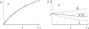
Fig. 11. Same as Figure 2, but for Siple core.

Fig. 12. Same as Figure 2, but for DE08 core.

It must be concluded that the correlations are not robust: correlations with similar errors can yield very different values of the proportionality factor, s _m, and consequently different patterns of the accumulation, . With this proportionality assumption it is the factor s _m that is not correctly determined by the age/depth correlations, and it appears that additional information, from the core data or otherwise, is needed to improve the choice of s _m. While independent and does not seem sensible, the above proportionality with uniform is likely to be too restrictive, and the situation allowing depth dependence of the strain rate is now being analysed. This is expected to require more core information.

Property Evolution

The knowledge of past conditions and particle paths for each element in the core is essential to relate current core measurements to growth laws which describe the evolution of different ice properties. Reference MorlandMorland (2009) considered relations for grain growth and dislocation density evolution for three cores, using data curves given by Reference De La Chapelle, Castelnau, Lipenkov and DuvalDe La Chapelle and others (1998) and Reference Montagnat and DuvalMontagnat and Duval (2000) to determine past independent accumulation and strain rate, in contrast to their assumption of unchanged past conditions. However, it was still assumed that the present temperature profile with depth had remained unchanged. While we have no reliable kinematic histories for the 11 cores analysed here, and no temperature history, we will present a general form of growth relation and illustrate how it is related to the histories of the core variables.

Grain growth depends, at least, on temperature and strain rate, and fabric evolution depends further on deformation. The most simple dependence is on second invariants of shear strain rate and shear strain, defined by

using Eqn (5) ₂, where the positive root of b is implied, and in the limit as λ → 1, from below or above:

Since the invariant b has a zero rate of increase with time at b = 0, it is not a useful monotonic parameter to describe initial changes. However, E increases strictly monotonically from zero as λ decreases from unity, and also in tension as λ increases from unity with s < 0. Further, in a simple shear γ, E = |γ|, which increases strictly from zero as |γ| increases from zero. E is therefore a sensible strain invariant measure.

Consider a property A satisfying a typical evolution relation for particle P:

where A _p(t _p) = A ₀, T is temperature, a(T) is a rate factor, ζ is one or more invariants such as I and E, and is a function of the property and collection of kinematic variables ζ. For example, could be a grain area or diameter squared when Eqn (23) is a grain growth relation. With determined by Eqn (11) ₁, E _p(t) by Eqns (21) and (11)₂, and I _p(t) by Eqn (20) in terms of s(t) for all past times during the core age, Eqn (23) can be integrated from each t _p to t = 0 to determine the distribution of down the present core. The age of particle P at time t is , which increases from 0 to as P descends from the surface to depth at t = 0. Thus P is identified by the present age point, , in the core, and with the assumption that the initial value is the same for all P, Eqn (23) can be written as

where and . Time runs from to 0 as ice with current age moves down from the surface to current depth, . The distribution of A down the present core is given by the solution of Eqn (24) at the end time, .

Temperature history is a significant ingredient of a growth relation (23) when the rate factor, a(T), varies strongly with T. This is a feature of ice where response rates decrease sharply as T falls significantly below the melting point. Neglecting the negligible shear stress working near a divide, the temperature is determined by the vertical energy balance

where λ _i = 7 × 10⁷ N K⁻¹ a⁻¹ is the thermal conductivity of ice and C _i = 2 × 10³ N m kg⁻¹ K⁻¹ is the specific heat of ice, subject to surface and bed boundary conditions, and an ‘initial’ (present time) distribution. Dimensionless analysis (Reference MorlandMorland, 1984) of the energy balance shows that all three terms have equal status, so the assumption that the present temperature distribution, say with depth, has remained steady in the past, adopted by Reference MorlandMorland (2009), is only a good approximation when T is uniform in z through the core, so that all derivatives are zero. A balance between advection and diffusion, to allow a zero temperature time derivative when not uniform in z, implies w is independent of t which, by Eqns (1) ₂ and (2), is only possible when conditions have remained unchanged. The corresponding age/depth relation (17) is not consistent with any of the core data studied. When T is not approximately steady, solutions of the coupled equations (24) and (25) are required, and property evolution becomes a more major problem.

Conclusions

Age/depth data from 11 ‘present’ ice cores have been used to infer past surface accumulation and vertical strain-rate histories, and hence the paths of the ice element at each depth since deposited at the surface, necessary to describe the evolution of ice properties during its descent down the core. The conventional assumptions of purely vertical motion and uniform vertical strain rate down the core have been made to yield a tractable one-dimensional analysis. The present correlations have assumed that strain rate is proportional to accumulation, in contrast to the earlier correlations for which they were treated as independent histories. It is found, however, that the correlations are not always robust; that is, correlations nearly as good as the best found, and shown, have quite different proportionality factors and consequently parameters in the accumulation, which give very different accumulation history patterns. It must be concluded that more core information is required to choose the best correct proportionality factor for this strain-rate assumption.