


Introduction
Calving is one of the largest sources of uncertainty in projected mass loss from ice sheets and glaciers (Stocker and others, Reference Stocker2013; Pörtner and others, Reference Pörtner2019; Pattyn and Morlighem, Reference Pattyn and Morlighem2020) and developing better models of the calving process is essential for accurate sea level projections. Current parameterizations of calving, such as height above buoyancy (Vieli and others, Reference Vieli, Funk and Blatter2001), eigencalving (Levermann and others, Reference Levermann2012) or von Mises stress (Morlighem and others, Reference Morlighem2016) can replicate behavior of glacier advance and retreat in some cases, but the predictions made by these parameterizations often have several tunable parameters and result in projections of rates of mass loss that diverge over time (Choi and others, Reference Choi, Morlighem, Wood and Bondzio2018).
The Nye zero stress criterion provides a simple method to introduce a physically motivated parameterization of calving into glacier models (Nye, Reference Nye1957; Nick and others, Reference Nick, Van der Veen, Vieli and Benn2010; Todd and Christoffersen, Reference Todd and Christoffersen2014; Ma and others, Reference Ma, Tripathy and Bassis2017; Ma and Bassis, Reference Ma and Bassis2019). This criterion assumes crevasses penetrate to the depth in the glacier where the largest effective principle stress vanishes. The Nye zero stress criterion has some disadvantages: it lacks coupling between flow and fracture and assumes closely spaced crevasses, which is a good assumption for Greenland outlet glaciers but less so for Antarctic ice shelves (Colgan and others, Reference Colgan2016). However, the method is computationally cheap to incorporate into models and straightforward to implement compared to other theories that can be cumbersome to include in ice-sheet models, such as linear elastic fracture mechanics (Krug and others, Reference Krug, Weiss, Gagliardini and Durand2014; Yu and others, Reference Yu, Rignot, Morlighem and Seroussi2017; Jiménez and Duddu, Reference Jiménez and Duddu2018).
However, with a few exceptions (Bassis and Ma, Reference Bassis and Ma2015; Sun and others, Reference Sun, Cornford, Moore, Gladstone and Zhao2017), previous crevasse depth studies omit the effect of crevasse advection despite the fact that observations show advection is important in predicting the location and depth of crevasses (e.g. Mottram and Benn, Reference Mottram and Benn2009; Hubbard and others, Reference Hubbard2021; Enderlin and Bartholomaus, Reference Enderlin and Bartholomaus2020). The omission of crevasse advection and the assumption that crevasses immediately ‘heal’ makes modeled calving solely dependent on the instantaneous stress within the glacier. Although instantaneous stress near the terminus may be diagnostic of criteria for calving in some cases, it may not adequately predict calving events where ice near the terminus is highly crevassed due to previous crevasse formation and advection.
An alternative approach to simulating fractures in ice uses damage mechanics, which can easily incorporate crevasse advection of a scalar (or tensor) damage variable (Pralong and Funk, Reference Pralong and Funk2005; Borstad and others, Reference Borstad2012; Duddu and others, Reference Duddu, Bassis and Waisman2013; Krug and others, Reference Krug, Weiss, Gagliardini and Durand2014; Jiménez and others, Reference Jiménez, Duddu and Bassis2017). Damage mechanics is well suited to simulate the propagation of crevasses within numerical models because it avoids complex remeshing of crevassed geometries. However, damage mechanics can be computationally expensive to implement for long timescale simulations. It also relies on empirical damage production criteria that are difficult to constrain with field or laboratory data, although model results may be relatively insensitive to parameter tuning in some cases (Duddu and others, Reference Duddu, Jiménez and Bassis2020).
Here, we formulate a calving model that combines elements of the Nye zero stress model with damage mechanics. The basis of our model is the Nye zero stress crevasse criterion. However, we generalize the Nye zero stress model to include advection of ‘damaged’ or crevassed regions of ice. Our implementation is computationally simple and has few tunable parameters. Although similar to damage based models, our model assumes that brittle failure occurs rapidly compared to the timescale of ice flow and thus portions of the ice transition immediately from ‘intact’ to ‘fractured’. This reflects the reality of the calving process: ice fractures near instantaneously compared to the time it takes for appreciable flow.
Flow model description
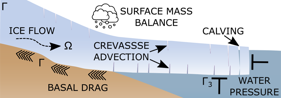
We include crevasse formation and advection in a 2-D flowline glacier model. Choosing a 2-D representation reduces computational cost and simplifies the implementation of the calving criteria. A schematic illustration of the model is shown in Figure 1. The different elements are described in detail below.

Fig. 1. Illustration of the different processes in the calving model. Incompressible flow with indicated boundary conditions determines the viscous evolution of the glacier. Based on the Nye zero stress criterion, tensile crevasses form and advect with the ice. A calving event occurs when surface and basal crevasses meet.
Incompressible viscous flow
We use a modified version of the incompressible equations describing slow, viscous flow, which can be written as:

where Ω indicates the entire glacier domain (Fig. 1). The effective viscosity is denoted by η, the ice density by ρ, the acceleration due to gravity by g, the velocity vector by u(x, z, t) and the pressure by p(x, z, t). We retain the acceleration term following Berg and Bassis (Reference Berg and Bassis2020) as a physically based regularization that avoids unphysical time-step dependence of the velocity and stress fields.
The effective viscosity of ice is calculated using Glen's flow law using a temperature-dependent constant B and a flow law exponent n = 3:

where the effective strain rate is related to the strain rate tensor by:

and we have used summation notation.
Boundary conditions
Denoting the ice divide boundary as Γ1 and the ice–bed interface as Γ2 (Fig. 1), the boundary conditions on velocity are given by:

where $\hat {n}$ is defined as the outward facing unit normal vector. The velocity boundary condition on Γ1 represents zero inflow at the ice divide. The inequality condition on Γ2 is a no-penetration boundary condition for grounded ice.
For simplicity, we use a modified Weertman sliding law with the drag force along the bed (Γ2) proportional to the cubed root of the sliding velocity. Defining Γ3 as the portion of the ice boundary beneath sea level (Fig. 1), the applied stresses for basal drag and water pressure are thus given by:

Here, $\hat {\tau }$ denotes the unit vector tangential to the surface, β is the sliding coefficient, ρ w is the density of water, z w is the ice depth relative to sea leveland σ is the Cauchy stress tensor.
Traction must also vanish at the ice divide (Γ1) and on the ice-ocean boundary (Γ3). On the ice-atmosphere boundary Γ4, there are no external stresses. These conditions are expressed as:

Model implementation details
Flow solver
We implement our model using the open source finite-element solver FEniCS with an arbitrary Lagrangian–Eulerian formulation using mixed Taylor–Hood elements with the second-order continuous Galerkin elements for velocity and first-order continuous Galerkin elements for pressure (Alnæs and others, Reference Alnæs2015; Helanow and Ahlkrona, Reference Helanow and Ahlkrona2018). We solve the incompressible flow equations (Eqn (1)) using Picard iterations with a linear solver and calculate the acceleration term in the momentum balance using a backward Euler step with a zero velocity initial condition to avoid an unphysical dependence of results on time-step size (Berg and Bassis, Reference Berg and Bassis2020). For all simulations we use a maximum time step of 3 days and restrict to a shorter time step if necessary based on the CFL (Courant-Friedrichs-Lewy) criterion with a Courant number of 0.5. Decreasing the time step does not affect results, indicating numerical convergence.
Boundary forces
We implement the no-penetration boundary condition (Eqn (4)) on grounded ice (Γ2) by adding an additional force on grounded ice. This force represents the elastic properties of subglacial rock and sediment and is numerically equivalent to a penalty method. This boundary condition is given by:

The elastic force is directly proportional to the distance under the bed that the ice has penetrated in the normal direction, where the location of the bed is denoted by rb, the location of the ice is r and α is the elastic coefficient. We use a value of 100 ${\hbox {kPa}}\, {\hbox {m}^{-1}}$ for the elastic coefficient. Our results are insensitive to the value of α over a wide range, and our chosen value agrees broadly with measurements of the Young's modulus of glacial till. Taking the Young's modulus of a loose glacial till to be 10 MPa (Bowles, Reference Bowles1996), our value for the elastic coefficient corresponds to a plausible glacial till thickness of 100 m (Walter and others, Reference Walter, Chaput and Lüthi2014).
For implementation of the elastic bed force and force due to water pressure (Eqns (5 and 7)), we introduce a damping term for vertical velocities to ensure that the ice displacement during flotation or rebounding from the bed is numerically stable. These damping terms are those of the form derived in Durand and others (Reference Durand, Gagliardini, De Fleurian, Zwinger and Le Meur2009), which result from a Taylor expansion in the vertical position dependence of the elastic and water pressure forces and includes dependence on the time step Δt and the unit vector in the vertical direction $\hat {z}$ :
:

Crevasse advection and calving
For crevasses to form, we assume that the local stress field must satisfy the Nye's zero stress criterion (Nye, Reference Nye1957). The largest effective principle stress $\sigma _{\hbox {Nye}}$ is defined using the greatest principle stress σ 1 as:

We model crevasse formation and advection as a binary scalar field of ‘crevasses’ in the ice. To advect crevasses in the model, we use massless tracers in a ‘particle-in-cell’ method and store the binary crevasse field independently from the finite-element mesh. Using tracers to advect properties limits numerical diffusion and allows us to resolve sharp changes separating regions that are crevassed from those that are not. We use LEoPart (Maljaars and others, Reference Maljaars, Richardson and Sime2020), an add-on to FEniCS that includes this functionality, to implement the particle-in-cell crevasse advection. Computational overhead using tracers is small and the time required to run our model is dominated by the Stokes flow solver. Additionally, our particle-in-cell implementation is convenient using LEoPart, but any numerical advection method can be used as long as results are not overly diffusive.
A set of tracers are randomly distributed throughout the domain with 32 tracers initially in each finite-element cell as shown in Figure 2. In general, more tracers increase the precision of results and results are converged with 32 tracers per cell. At each time step, the diagnostic stress is projected to a first-order discontinuous Galerkin space and then evaluated at the tracer locations to determine if new crevasses form. Similarly, the velocity solution on a second-order continuous Galerkin space is evaluated at the tracer locations to advect their position.

Fig. 2. Computational representation of the model glacier near the calving front. The unstructured finite-element mesh is shown in black. Gray dots within the mesh show the random distribution of tracers. Initially, tracers are distributed so that each finite-element cell has 32 tracers. As tracers advect with the mesh, tracers are added so that a minimum of 32 tracers are maintained in each cell.
Using coordinates (x i, z i) to denote the position of the ith tracer at time τ, the crevasse field c i(τ) at the nth time step is given by:

This implementation of the Nye's zero stress criterion is equivalent to the choice of a zero tensile yield strength for ice. One limitation of our approach is that we do not resolve individual crevasses, but instead consider a macroscopic ‘field’ where regions are either fractured or intact. Moreover, our crevasse criterion effectively introduces a binary damage parameter that is zero or unity. This implies that the timescale of damage growth is fast compared to the viscous timescale. For this study, we assume crevasses are narrow brittle features that do not affect the larger-scale rheology.
Once formed, crevasses persist indefinitely and, in our model, are not allowed to heal. Extended time under compressive stress may allow crevasses to close and refreeze. However, we assume that even if crevasse do close, they remain weak planes that are prone to reactivating under appropriate stress conditions.
After every time step, we analyze the stress field using a method inspired by Todd and Christoffersen (Reference Todd and Christoffersen2014). We generate a contour of crevassed ice based on the binary scalar crevasse field stored on the tracers. This contour indicates where the ice transitions from crevassed to intact. In places where the contour indicates crevasses penetrate the entire glacier, we assume a vertical fracture and remove all calved ice. We restrict calving to occur along vertical planes of the glacier during tensile failure for simplicity, but could specify non-vertical calving planes given an appropriate criterion to determine the angle of the exposed calving face.
After a calving event we remesh and add tracers to the domain randomly to maintain a minimum of 32 tracers per cell. Tracers are initialized by interpolating existing tracers using LEoPart functionality. Figure 3b shows a snapshot of the crevasse field during a modeled calving event with crevasse advection and the location of calving based on our criteria. In our implementation, calved ice ‘vanishes’ and does not provide any back stress after detachment from the glacier, neglecting the effect of mélange.

Fig. 3. Snapshot of floating ice tongue with purple showing crevassed ice and vertical calving indicated by a dashed white line. Model results shown without crevasse advection (a) and with crevasse advection (b). Slippery bed parameters as given in Table 1. Crevasses advecting from the grounding line to the calving front lead to a calving event if advection is included. After a calving event occurs, all calved ice is removed and is no longer present in the model.
Table 1. Set of parameters used for model tests

Meshing
We use the external remeshing package Gmsh (Geuzaine and Remacle, Reference Geuzaine and Remacle2009) for remeshing of the domain. Using Gmsh, we have precise control over the meshing process and break the glacier into high-resolution and low-resolution subdomains. Dividing the glacier into high-resolution and low-resolution regions allows us to simulate the entire glacier and maintain the ice divide boundary condition (Eqn (4)) while avoiding excessive computation time. We use an initial mesh size of 10 m in the high-resolution region and a mesh size of 100 m in the low-resolution region, with the high resolution region starting five ice thicknesses toward the ice divide from the grounding line. Model results are insensitive to changes in the low-resolution mesh size and converged with high resolution mesh size such that sizes smaller than 10 m do not significantly change results. We remesh after every calving event or when the ratio of minimum to maximum finite-element cell radii drops below a threshold of 0.1 according to the built in FEniCS mesh quality class.
Suite of tests
To test the effects of crevasse advection on calving behavior in different environments, we first ran the model on a set of parameters with different ice temperatures and sliding coefficients. This initial suite of simulations all have a constant prograde bed slope of 0.01 broadly based on average bed slopes of Svalbard glaciers (Dunse and others, Reference Dunse, Schuler, Hagen and Reijmer2012). Ice temperature and sliding temperature parameter sets are listed in Table I in four different combinations: baseline, warm ice, slippery bed and warm ice and slippery bed. A constant surface mass balance of 0.25 m a−1 is applied in all cases, a moderate value broadly appropriate for, e.g. the Austfonna Ice Cap (Schuler and others, Reference Schuler2007).
Ice temperature
We use a moderate temperature of −10°C as our baseline temperature, roughly corresponding to near surface temperatures on Jakobshavn Isbræ (Iken and others, Reference Iken, Echelmeyer, Harrison and Funk1993; Lüthi and others, Reference Lüthi, Funk, Iken, Gogineni and Truffer2002) and modeled ice temperatures of the Austfonna Ice Cap (Østby and others, Reference Østby, Schuler, Hagen, Hock and Reijmer2013). To investigate the case of warmer ice we use a temperature of −2°C, which agrees with modeled melt season temperatures at Austfonna (Harrington and others, Reference Harrington, Humphrey and Harper2015). The Glen's flow law coefficient B was taken for each temperature from the values given by Hooke (Reference Hooke2005).
Sliding coefficient
We use a baseline sliding coefficient of $7.6 \times 10^{6} \, \hbox {Pa} \, \hbox {m}^{-{1}/{3}} \, \hbox {s}^{{1}/{3}}$ , which is identical to the coefficient used for the modified Weertman sliding law in the Marine Ice Sheet Intercomparison Project (MISMIP) (Pattyn and others, Reference Pattyn2012). Although previous studies on Svalbard glaciers have a preference for a linear sliding law, those studies obtain linear drag coefficients on the order of 109–$10^{11} \, \hbox {Pa} \, \hbox {m}^{-1} \, \hbox {s}$
 (Schäfer and others, Reference Schäfer2012; Vallot and others, Reference Vallot2017; Gong and others, Reference Gong2017). The high end of that range is consistent with the sliding coefficient of $7.2082 \times 10^{10} \, \hbox {Pa} \, \hbox {m}^{-1} \, \hbox {s}$
 used for linear sliding law tests in MISMIP to achieve similar sliding velocities as the modified Weertman sliding law tests. Because this is a fairly high sliding coefficient, we halve the coefficient to see the effects of a more slippery bed.
Bed with a sill
In addition to the ice temperature and sliding coefficient tests, we also perform tests on a prograde bed with an idealized sill to investigate the combination of varying bed topography and crevasse advection on calving behavior. In this case, we superimpose a Gaussian bump with amplitude 25 m and SD 50 m on the 0.01 slope constant prograde bed 250 m ahead of the initial calving front. This is broadly consistent with spatial variation of bed geometry near the calving front of some Svalbard glaciers (Nuttall and others, Reference Nuttall, Hagen and Dowdeswell1997; Dunse and others, Reference Dunse, Schuler, Hagen and Reijmer2012; Dumais and Brönner, Reference Dumais and Brönner2020).
Variations on bed slope
To examine the effect of varying bed slope, we perform three additional tests with our ‘baseline’ parameter set with different bed geometries. Two tests are constant prograde slopes of 0.005 and 0.02, which correspond to half and double the previously used slope, respectively. And third, we run the model on a bed geometry with a retrograde slope near the calving front. This bed geometry has a constant prograde slope of 0.01 from the ice divide to 1 km from the initial glacier terminus. For the final 1 km, the bed is retrograde with a slope of 0.0025.
Initial conditions
We initialize the ice surface to a constant slope identical to the bed slope and constant thickness of 200 m from the ice divide boundary to the terminus at 50 km, roughly consistent with geometry of Svalbard outlet glaciers (Dunse and others, Reference Dunse, Schuler, Hagen and Reijmer2012). From the initial ice configuration we run the model with the calving front held fixed at its initial location (assuming a calving rate that exactly balances the velocity at the calving front) until the ice relaxes to a steady state (2500 years). Once the glacier has reached steady state, we allow the ice to flow and advance an additional 0.5 years before allowing crevasses to initiate using the Nye zero stress criterion. The extra 0.5 year relaxation avoids any artifacts associated with initializing the model with a vertical calving face. We start all simulations without any crevasses and perform all simulations with and without advection of crevasses.
Results
Crevasse advection increases calving
We first examined the effect of crevasse advection on terminus position using a prograde bed without a sill and varying ice temperature and sliding coefficient. Figure 3 shows snapshots illustrating initial ice tongue advance with and without crevasse advection on a slippery bed. Without crevasse advection (Fig. 3a), bending near the calving front results in a compressive stress at the grounding line that prevents basal crevasse formation. However, with crevasse advection (Fig. 3b), basal crevasses that initiate before the grounding line advect past the grounding line, resulting in a crevassed region that penetrates the entire thickness 300 m from the calving front. This effect is shown over time in Animation S1. Crevasse advection causes increased calving frequency and decreased glacier length relative to when advection is omitted.
The cumulative effect of the increased calving frequency is illustrated in Figure 4, which shows the change in glacier length over time relative to initial grounding line position for the suite of scenarios. In the baseline parameter tests (Figs 4a, e), crevasse advection makes little difference to glacier terminus position. However, when we decrease the sliding coefficient (more slippery bed) or increase ice temperature (warmer ice, Fig. 5), we see crevasse advection has a larger effect on terminus position. For example, in all tests that have warmer ice or a lower sliding coefficient (Figs 4f–h), the ice tongue disintegrates, resulting in a grounded calving cliff. The warmer ice and slippery bed conditions are broadly representative of Greenland glaciers, few of which form ice tongues (Rignot and Kanagaratnam, Reference Rignot and Kanagaratnam2006; Hill and others, Reference Hill, Carr, Stokes and Gudmundsson2018).

Fig. 4. Glacier length change over time relative to initial grounding line position without crevasse advection (a–d) and with crevasse advection (e–h) for baseline parameters (a, e), slippery bed (b, f), warm ice (c, g) and both slippery bed and warm ice (d, h). Grounding line is plotted only when the glacier terminus is floating. The inclusion of crevasse advection causes ice tongue disintegration for three of the parameter sets. The effect of crevasse advection on terminus position is most pronounced for warmer ice, where we observe retreat and then stabilization of the calving front for approximately a decade before re-advance.

Fig. 5. Glacier evolving in time without crevasse advection (a–c) and with crevasse advection (d–f). Warm ice parameters as given in Table I. Without crevasse advection, the ice tongue grows and advances over time. Crevasse advection increases calving, leading to ice tongue disintegration followed by stabilization of calving front position for approximately a decade. At the end of simulation, the grounded calving cliff has started to re-advance.
When the ice tongue disintegrates, we find that crevasses formed before the grounding line when the ice tongue was intact persist, resulting in transient calving behavior until these crevasses advect out of the system. For example, Figure 6 shows crevasses and the Nye stress after ice tongue disintegration for warm ice. The Nye stress is insufficient to cause full penetration of crevasses near the calving front. Uncrevassed regions exist at the base of the glacier and near the surface. However, with crevasse advection, existing crevasses take time to move through the domain resulting in a transient period of increased calving that can last a few years to a decade.

Fig. 6. Glacier crevasses (a) and Nye stress (b) after ice tongue collapse, 2 years after start of simulation. Warm ice parameters as given in Table 1. The contour of zero Nye stress is indicated by a dashed black line, indicating regions of newly crevassed ice. Current Nye stress is insufficient for full penetration of crevasses. However, crevasses developed when the glacier had an ice tongue are present and cause further calving.
Crucially, the contribution of crevasse advection is most pronounced for our test with warm ice (Figs 4f, 5, Animation S2). Glacier retreat continues after ice tongue disintegration and results in a stable grounded calving front position retreated from the initial calving front for approximately a decade (Fig. 5e) before the glacier starts to readvance (Fig. 5f). This temporary retreat followed by re-advance is observed in the other tests but is shorter: ~2 years with a slippery bed (Fig. 4g, Animation S1) and under a year for warm ice with a slippery bed (Fig. 4h). In the slippery bed simulations, increased flow velocity rapidly exports transient basal crevasses away from the grounding line. In the warm ice with a slippery bed case, the short ice tongue disintegrates quickly and is not able to form basal crevasses near the grounding line. These results hint that glacier calving behavior is not solely a consequence of immediate forcing and suggests glacier advance or retreat could be dependent on earlier conditions.
Surprisingly, in no case do we observe sustained glacier retreat regardless of ice temperature or sliding coefficient. Instead, glaciers either advance or temporarily retreat before re-advancing.
Stabilizing behavior of sill
Because several glaciers stabilize on sills near the terminus, we performed simulations using our baseline parameter set with a bump in the bed. In tests with and without crevasse advection, when the ice tongue is forced over the sill, high bending stresses at the grounding line cause a large calving event that removes the ice tongue. The newly formed grounded ice cliff advances again toward the sill. As shown in Figure 7, after a few large calving events, both tests achieve steady behavior after ~30 years. Glacier evolution for a total of 50 years is shown in Animation S3.

Fig. 7. Glacier length change over time relative to initial grounding line position without crevasse advection (a) and with crevasse advection (b) for a constant prograde bed with a Gaussian bump 250 m ahead of the glacier starting position. Brown dashed line indicates location of the sill. Baseline parameters as given in Table I. Grounding line is plotted only when the glacier terminus is floating. Both tests have a transient period characterized by large calving events before settling into steady behavior after ~30 years. With crevasse advection, the sill strongly inhibits glacier advance, leading to a stable calving cliff. Without crevasse advection, an ice tongue forms and periodically calves, giving a stable grounding line at the sill.
Without crevasse advection, Figure 7 shows that the glacier advances over the sill and forms a short ice tongue. The tongue periodically disintegrates from increasing stress at the top of the calving front as the ice tongue advances. Thus, even in the absence of crevasse advection, bed geometry can have a strong effect on glacier advance. However, without crevasse advection, the glacier retains a short floating ice tongue that may provide some protection against perturbations in ocean forcing.
In contrast, when crevasse advection is included, Figure 7 shows that the sill strongly inhibits advance and the glacier forms a stable calving cliff at the location of the sill. As the glacier advances over the bump in the bed, a higher cliff and the concave bed shape increase stresses. Advected crevasses caused by these higher stresses inhibit advance over the sill. We also observe brief periods where the glacier temporarily retreats to the base of the sill before re-advancing at ~37 years, 42 years and 47 years. This behavior is caused by slowly advecting surface crevasses at the top of the calving cliff that eventually meet with basal crevasses and cause a more significant calving event.
The resulting calving front is qualitatively similar to Store Glacier in Greenland, which terminates at a bump in the bed (Todd and Christoffersen, Reference Todd and Christoffersen2014). Store Glacier exhibits ice front advance and retreat coinciding with the presence of seasonal ice mélange (Howat and others, Reference Howat, Box, Ahn, Herrington and McFadden2010), with our crevasse advection results showing behavior similar to Store glacier in the absence of additional mélange back stress.
In our simulations, glaciers advance on a prograde bed until they reach a bump in the bed where they can stabilize. This is analogous to the behavior of most stable glaciers that remain perched on sills, but our model still fails to reproduce sustained retreat. To explore if this is a general result indicating a failure of the Nye zero stress model or a consequence of the particular geometry, we explored a larger range of bed slopes.
Bed slope combined with crevasse advection changes calving behavior
Finally, we examined the effect of increasing or decreasing the bed slope. Adjusting the bed slope changes the flow velocity, but in the absence of crevasse advection we see no change in calving behavior (Figs 8a–c). All cases result in continuous glacier advance with negligible calving for all slopes tested. This is consistent with results in Figures 4a–d using a constant prograde slope of 0.01.

Fig. 8. Glacier length change over time relative to initial grounding line position with crevasse advection (a–c) and with crevasse advection (d–f) for baseline parameters with a half prograde slope (a, d), double prograde slope (b, e) and retrograde slope (c, f). Grounding line is plotted only when the glacier terminus is floating. With a lower bed slope, significant calving does not occur regardless of crevasse advection. However, including crevasse advection causes significant calving with a higher prograde slope and with a retrograde slope. Both the double prograde slope and retrograde slope tests experience a period of relative steady-state terminus position for ~2 years and then transition into a period of gradual retreat for the remainder of simulation.
With a halved bed slope (Fig. 8d), the change in calving rate due to crevasse advection is negligible as in the initial baseline test (Fig. 4e). This test has reduced ice velocities and lower strain rates that cause less crevasse formation. The percentage of time that a grounding line is present is reduced over 10 years of simulation, showing again that crevasse advection discourages ice tongue formation. However, the overall rate of terminus advance remains nearly identical.
With a doubled prograde slope (Fig. 8e) and a retrograde slope (Fig. 8f), crevasse advection plays a critical role in calving behavior and causes a significant retreat. Moreover, both tests show similar calving behavior over the 10 years of simulation. For the first 2 years, advance is stagnant and there is an approximately steady terminus position. However, with crevasse advection, crevasses form several hundred meters before the calving front and then advect, eventually allowing full crevasse penetration through the glacier. After a period of crevasse accumulation, constant retreat begins. This initially observed ‘steady-state’ behavior is transient as crevasses initially form and advect through the domain.
Discussion
In our suite of tests, advection of crevasses overall increases calving rates and reduces the rate of terminus advance. This effect is pronounced and significant, given that without crevasse advection, only our test with a sill shows any significant calving behavior. One of our most significant results is that when crevasse advection is included, glacier behavior depends on the history of crevasses in the glacier. This suggests some care in interpreting observations of glacier retreat as calving and the crevasse distribution may include a transient response to events that occurred years or even decades earlier.
The magnitude of the calving increase due to crevasse advection is dependent on a range of physical parameters including ice temperature, sliding coefficient and bed geometry. All of these parameters change the ice flow velocity and therefore also affect the rate at which crevasse advect through the domain and the ice geometry. Changing geometry, such as varying cliff height at the calving front can significantly alter stresses within the ice and affect crevasse formation.
In contrast to tests without crevasse advection, where we primarily observe steadily advancing glaciers, results with crevasse advection show a wide range of behavior depending on chosen parameters: advance, temporary retreat, sustained retreat and steady-state behavior. However, our model does not include other mechanisms that would also change the rate of terminus advance. One such omission is submarine melt. Submarine melt rates vary over a wide range. For example, estimated values in Hansbreen, Svalbard span the range from 0 to 15 m week−1 (De Andrés and others, Reference De Andrés2018), which would strongly contribute to total mass loss given that our model flow velocities are in the range of 1–5 m week−1. The inclusion of submarine melt could cause glacier retreat without crevasse advection, but we would expect experiments with crevasse advection to experience a reduction in terminus velocity as well.
Furthermore, the reduction in terminus velocity with crevasse advection would not necessarily be a simple superposition of previous calving rate and new melt rate. Calving rates for Svalbard glaciers are strongly dependent on ocean temperature (Luckman and others, Reference Luckman2015) and previous modeling has demonstrated that relatively small melt rates can promote calving (Ma and Bassis, Reference Ma and Bassis2019) – an effect that could be magnified with the inclusion of crevasse advection. A melt profile focused on the grounding line reduces glacier thickness and promotes a buoyant transition. This could increase the contribution of crevasse advection to calving rates given that the deepest advected crevasses are near the grounding line where the ice transitions to flotation.
However, in addition to processes that may increases overall mass loss, our model also lacks some mechanisms that may stabilize calving retreat. For example, we do not include coupling between crevasses and the ice rheology. Given that we treat crevasses as a scalar field, it would be possible define a damage variable as a function of the crevasse field and couple it to the ice rheology in a similar manner to that of Sun and others (Reference Sun, Cornford, Moore, Gladstone and Zhao2017). Coupling of crevasses with the rheology may decrease cliff heights, reducing stress and the potential for retreat. However, a different rheology could affect crevasse formation as well. If viscosity decreases as ice becomes crevassed, ice may fail more easily under tensile failure. This could increase the effect of crevasse advection on calving behavior.
Another possible contributor to stabilization is backstress due to calved mélange rather than instantaneously removing all calved ice from the model domain. Back stress from mélange has been shown to have significant effects on calving behavior (Joughin and others, Reference Joughin2012; Todd and Christoffersen, Reference Todd and Christoffersen2014; Bassis and others, Reference Bassis, Berg, Crawford and Benn2021). For a rapidly retreating grounded ice cliff, the rapid buildup of mélange could provide significant stabilizing stress and potentially stop collapse.
Finally, the lack of crevasse healing is a key assumption in our model. Crevasses in tests without advection instantaneously heal while crevasses in tests with advection persist indefinitely. Allowing crevasse healing could produce calving rates between those limiting cases. However, it remains unclear if healed crevasses remain weak or regain their original strength. Moreover, calving in our model is dominated by crevasses formed near the grounding line or calving front and these crevasses do not have significant time to heal. Nonetheless, by comparing model predictions to field observations it may be possible to assess the role of crevasse healing in calving.
Conclusion
Crevasse advection, which is easily included in existing Nye-based crevasse parameterizations of calving, can play an important role in controlling model (and perhaps glacier) behavior. This is especially important because phases of retreat and advance are not necessarily instantaneously connected with climate forcing. Instead, we anticipate a response time comparable to the time it takes crevasses to advect through the domain. This may aid in explaining some of the confusion in attributing glacier retreat to atmospheric or oceanic forcing.
Our results also show that – at least for the geometries we considered – simulated glaciers rarely retreat in the absence of crevasse advection. Including crevasse advection reduces the overall rate of advance by increasing calving and also leads to transient behavior. This effect is more pronounced with warmer ice.
Crevasse advection also increases the importance of basal topography. When crevasse advection is included, we see a transition to retreat when bed slope is increased. When approaching a sill in the bed, crevasse advection contributes strongly to calving events and prevents further advance, leading to a stable ice cliff rather than a transient ice tongue.
Our study points to the important role that crevasse advection can play in calving behavior. Future attempts to model the calving process need to carefully disentangle the instantaneous effect of crevasse opening versus the more subtle effect of the transport of crevasses from regions of higher stress to regions of lower stress.
Supplementary material
The supplementary material for this article can be found at https://doi.org/10.1017/jog.2022.10.
Acknowledgements
We thank the scientific editor Ian Hewitt and two anonymous reviewers for their valuable feedback on this manuscript. This study is from the DOMINOS project, a component of the International Thwaites Glacier Collaboration (ITGC). Support from National Science Foundation (NSF: Grant 1738896) and Natural Environment Research Council (NERC: Grant NE/S006605/1) is acknowledged. Logistics provided by NSF-U.S. Antarctic Program and NERC-British Antarctic Survey. ITGC Contribution No. ITGC-041. Code to run the tests in this paper is available at https://doi.org/10.5281/zenodo.5899711 (Berg, Reference Berg2022).


 Open access