


Introduction
Over 80% of glaciers in mid- to low-latitude mountain ranges are smaller than 0.5 km2 (Pfeffer and others, Reference Pfeffer2014). These very small glaciers contribute significantly to current sea level rise (Radić and Hock, Reference Radić and Hock2011; Zemp and others, Reference Zemp2019), and play an important role in local hydrology. However, in situ long-term mass-balance measurements are often restricted to large and medium size mountain glaciers (Gärtner-Roer and others, Reference Gärtner-Roer, Nussbaumer, Hüsler and Zemp2019; Zemp and others, Reference Zemp2019) and smaller glaciers are understudied in comparison (Fischer, Reference Fischer2018). Paul and others (Reference Paul, Kääb, Maisch, Kellenberger and Haeberli2004) suggest that localized down-wasting processes rather than a common dynamic response to climatic changes drive individual glacier change for many Alpine glaciers, and highlight that response variability is large particularly for smaller glaciers. Hence, extrapolating observations of mass balance or flow velocity from monitoring sites – typically larger valley glaciers – to neighbouring glaciers that differ in terms of size, aspect, slope or other characteristics is not straightforward. Ablation values, flow velocities and the contribution of reduced ice flow to overall loss differ depending on each glacier's characteristics. In the following, we refer to glaciers with an area <0.5 km2 as ‘very small’ and glaciers between 0.5 and 1 km2 as ‘small’ (Fischer, Reference Fischer2018; Leigh and others, Reference Leigh2019) unless otherwise noted.
Highly variable rates of surface elevation change and ice flow velocity at glaciers within the same mountain range as well as between neighbouring regions have been reported from around the world (Debeer and Sharp, Reference DeBeer and Sharp2007; Narama and others, Reference Narama, Kääb, Duishonakunov and Abdrakhmatov2010; Fischer and others, Reference Fischer, Huss and Hoelzle2015c; King and others, Reference King, Quincey, Carrivick and Rowan2017; Meier and others, Reference Meier, Grießinger, Hochreuther and Braun2018; Robson and others, Reference Robson2018; Menounos and others, Reference Menounos2019). Whether and how loss rates correlate with glacier size differs between regions: Lower rates of ice loss at small and very small glaciers compared to larger glaciers have been observed for the Canadian Rockies (Debeer and Sharp, Reference DeBeer and Sharp2007) and Glacier National Park (USA) (Menounos and others, Reference Menounos2019). Similarly, Abermann and others (Reference Abermann, Lambrecht, Fischer and Kuhn2009) found that the retreat of small glaciers in the Austrian Ötztal has decelerated compared to larger glaciers. In contrast, a comprehensive inventory of glaciers in Patagonia indicates that on average, relative ice loss is greatest for the smallest size classes in this region for the period 1986–2016, as well as since the LIA maximum (Meier and others, Reference Meier, Grießinger, Hochreuther and Braun2018). Meier and others (Reference Meier, Grießinger, Hochreuther and Braun2018) also note that some small glaciers do not show a noticeable decline between 1986 and 2016. Fischer and others (Reference Fischer, Huss and Hoelzle2015c) analysed the correlation between geodetic mass balance and several geometric parameters for all Swiss glaciers from 1980 to 2010, showing that there is high variability between individual glaciers and that the relation between mass balance and glacier geometry and hypsometry is complex. While some correlation was found for median elevation as well as the slope angle over the lowermost parts of the glacier, glacier size was on average not well correlated with mass balance, although some glaciers in the smallest size class (<0.1 km2) did show less negative mass balance values than larger glaciers.
In Austria – as well as in other mountain regions where very small glaciers dominate in number – local topography is considered the main factor determining the variable nature of the changes at individual glaciers under the same larger scale climatic forcing (Abermann and others, Reference Abermann, Kuhn and Fischer2011; Fischer and others, Reference Fischer, Huss and Hoelzle2015c; Florentine and others, Reference Florentine, Harper and Fagre2020). In particular, small and very small glaciers that exhibit lower rates of loss than the regional average typically do so due to favourable local topography and topography driven micro-meteorological processes (Kuhn, Reference Kuhn1995). DeBeer and Sharp (Reference DeBeer and Sharp2009) found no observable area change for 75 very small glaciers in their study region in the Monashee Mountains (British Columbia, Canada) and similarly attributed this to a mixture of topographic effects that lead to increased accumulation through avalanching or wind drift, and/or to decreased ablation due to shading. Florentine and others (Reference Florentine, Harper and Fagre2020) assessed the role of different terrain factors for the persistence of the mostly small and very small glaciers in Glacier National Park (USA) since the Little Ice Age. Using a multivariate analysis, they found that a substantial part of the variance could be explained by avalanche processes and exposure to solar radiation, and that some glaciers were able to persist to present times due to favourable wind exposure. Changes in debris cover also affect local variability in glacier responses: Mölg and others (Reference Mölg, Bolch, Walter and Vieli2019) showed that increasing debris cover at their study site in Switzerland affects the spatial pattern of elevation change but does not influence the overall magnitude of the glacier-wide change. In a case study of Tsarmine glacier, a very small glacier in Switzerland, Capt and others (Reference Capt, Bosson, Fischer, Micheletti and Lambiel2016) highlighted that highly debris-covered sections are less climate-sensitive than debris-free sections and that the overall response of the glacier to climate forcing is likely shaped by a combination of debris cover, solar exposure, snow redistribution and local permafrost conditions. In a regional study for Austria, Fleischer and others (Reference Fleischer, Otto, Junker and Hölbling2021) found significant increases of debris cover between 1996 and 2015 but report little impact of changing debris cover on overall regional melt rates.
Huss and Fischer (Reference Huss and Fischer2016) found that Swiss glaciers smaller than 0.5 km2 lost 60% of their total volume between the 1980s and 2010. The same study showed that the sensitivity of very small glaciers to climate change is similar to that of larger glaciers, but that there is large variability in individual responses. Huss and Fischer (Reference Huss and Fischer2016) expect most of the glaciers smaller than 0.5 km2 in 2010 (Fischer and others, Reference Fischer, Huss, Barboux and Hoelzle2014) to disappear in the coming decades but identified a few that may survive at reduced size beyond 2050, suggesting that the high variability between individual glaciers makes it challenging to delineate the response of individual glaciers to a common climate forcing.
In Austria, 90% (834 of 921) of glaciers are smaller than 1 km2, covering 35% of the country's total glacier area (Fischer and others, Reference Fischer, Seiser, Waldhuber, Mitterer and Abermann2015b). In total, 82% (757) are smaller than 0.5 km2, accounting for 23% of glacier area. The overall contribution of the many small and very small glaciers to total glacier area is greater than that of the few remaining large glaciers: Two glaciers in Austria are larger than 10 km2 and together account for 8% of Austrian glacier area. Between 1969 and 2018, the number of glaciers in the small and very small size classes has significantly increased as larger glaciers have disintegrated. Small and very small glaciers in Austria have lost between 25 and 50% of their volume between 1997 and 2006 (Helfricht and others, Reference Helfricht, Huss, Fischer and Otto2019).
While the overall trends in Austria and elsewhere are clear, the temporal and spatial characteristics of changes at the scale of individual glaciers are often ‘averaged out’ in regional studies: The wealth of information in the topographic and inventory data sets is such that a ‘big picture’ overview cannot resolve all the details contained in the data. In order to accurately track glacier changes and, in a further step, predict future changes and the numerous local to regional processes that are linked to glacier recession or even deglaciation, a broad overview of regional trends is important. To assess future glacier extent, the general trend as well as the variability of glacier responses within a region has to be taken into account. As glaciers change over time, individual response patterns may also change. Accordingly, to understand the overall variability in responses and controls thereof, how responses change over time must also be understood. Tracking responses and possible changes in responses at a glacier-individual level is important at the local scale to assess, e.g. future developments in individual catchments, and contributes to a more complete understanding of variability at the regional scale.
As a step towards assessing local variability of glacier change within the context of broader, regional trends, we present a methodological experiment with machine learning-based data analysis. Using a self-organizing maps (SOM) algorithm (Kohonen, Reference Kohonen2001), we identify recurring patterns of surface elevation change at individual glaciers, drawing on previous glacier inventories (GI) and recent survey data for western Austria. The SOM serves as a clustering technique, which allows grouping glaciers into types of similar surface elevation change distribution profiles, highlighting common patterns and how they change over time. The SOM is trained on data from the Ötztal range in Tyrol, one of Austria's most heavily glacierized regions. We then apply the trained SOM algorithm to the nearby Stubai and Silvretta mountain ranges, assessing how patterns differ between the different ranges.
In our study area in western Austria, digital elevation models (DEMs) and detailed GI data from multiple years form a rich data basis that complements data from monitoring sites by providing an overview of glacier change on a regional scale. The availability of repeat high-resolution elevation data and comprehensive inventories makes the region an ideal test case for developing monitoring strategies specifically for small mountain glaciers.
The main aim of this study is to explore the potential of the SOM algorithm for providing new perspectives on existing data of recent glacier thickness change. The results of the clustering analysis improves our understanding of the state of glaciers in western Austria on a regional scale, while preserving the characteristics of individual glaciers at a relatively high level of detail, which may contribute to a more refined understanding of the drivers of such variability in the future.
Data/methods
Geospatial data
This study is based on the geospatial data compiled by the first, second and third Austrian GI. In addition, more recent elevation data are available to complement the established inventories in certain regions. Results and methodology related to the compilation of GI1 can be found in Patzelt (Reference Patzelt1980) and Groß (Reference Groß1987) (Data publication: Patzelt, Reference Patzelt2013). For details on GI2 and the digitization of GI1 we refer to Eder and others (Reference Eder, Würländer and Rentsch2000), Lambrecht and Kuhn (Reference Lambrecht and Kuhn2007) and Kuhn and others (Reference Kuhn, Lambrecht, Abermann, Patzelt and Groß2012) (Data publication: Kuhn and others, Reference Kuhn, Lambrecht and Abermann2013). The DEMs used to map glacier boundaries in GI1 and 2 were generated from orthophotographs. GI1 represents the state of Austrian glaciers in 1969. The glacier boundaries of GI2 represent 1998. The acquisition of the orthophotos for the underlying GI2 DEM took place between 1997 and 2002 and glacier boundaries were homogenized for a common year during the compilation of this inventory (Lambrecht and Kuhn, Reference Lambrecht and Kuhn2007). GI3 was compiled based on airborne laserscanning (LiDAR - Light Detection and Ranging) derived DEMs acquired between 2004 and 2006 in the study area, and corresponding mapping of glacier boundaries. Details on GI3 and the underlying DEMs can be found in Abermann and others (Reference Abermann, Lambrecht, Fischer and Kuhn2009), Abermann and others (Reference Abermann2010b), Stocker-Waldhuber and others (Reference Stocker-Waldhuber, Wiesenegger, Abermann, Hynek and Fischer2010) and Fischer and others (Reference Fischer, Seiser, Waldhuber, Mitterer and Abermann2015b) (Data publication: Fischer and others, Reference Fischer, Seiser, Stocker-Waldhuber and Abermann2015a). For the Ötztal, Stubai and Silvretta regions, more recent LiDAR DEMs for 2017/18 (exact data acquisition dates differ by region) and glacier boundaries are available from survey campaigns carried out by the state government of Tyrol and Vorarlberg, respectively, and subsequent glaciological mapping. The DEMs are co-registered to the Austrian national grid. Details on DEM generation from the LiDAR data can be found in the reports on the survey campaigns by the respective federal government agencies (Federal Government of Tyrol, 2011; Landesvermessungsamt Feldkirch, Reference Landesvermessungsamt Feldkirch2004) and we refer to Fischer and others (Reference Fischer, Seiser, Helfricht and Stocker-Waldhuber2021) for a description of the glacier boundary mapping process.
To ensure consistency in raster-based computations, the more recent, high-resolution LiDAR DEMs were resampled to a resolution of 5 × 5 m to match the DEMs of GI1 and 2. Difference rasters were computed for each available time period by subtracting consecutive DEM pairs. In order to compare periods of different length, elevation differences in meters per year were computed by dividing by the length of the time period between DEMs on a pixel-wise basis, thereby accounting for different acquisition times. The data were processed using python and QGIS (Harris and others, Reference Harris2020; Hunter, Reference Hunter2007; McKinney, Reference McKinney2010; QGIS.org, Reference QGIS.org2010; Jordahl and others Reference Jordahl2020; Gillies and others, Reference Gillies2013). For the Ötztal and Stubai range, time period 1 refers to 1969–1997, period 2 refers to 1997–2006 and period 3 refers to 2006–2017/18. For the Silvretta region, the years of DEM acquisition differ slightly, see Table 1.
Table 1. Years of DEM acquisition for inventory surveys of the Ötztal, Stubai and Silvretta ranges

The Silvretta range is partially located in the state of Tyrol and partially in the state of Vorarlberg, and the two states were surveyed in different years: Survey 3 was carried out in 2004 in Vorarlberg and in 2006 in Tyrol, respectively. Survey 4 was carried out in 2017 in Vorarlberg and in 2018 in Tyrol, respectively. The 2017/18 DEM of Stubai is incomplete because the survey flights did not cover the eastern part of the range. ‘Area’ indicates the total glacierized area per range in the respective inventory year and ‘>1 km2’ gives the percentage of glaciers larger than 1 km2 per range.
The DEM underlying GI1 was digitized from analogue maps (Patzelt, Reference Patzelt1980). Eder and others (Reference Eder, Würländer and Rentsch2000) generated the GI2 DEM with a requirement of being able to resolve vertical differences since GI1 of 0.1 m per year. The year of data acquisition for GI2 varied depending on the region (Lambrecht and Kuhn, Reference Lambrecht and Kuhn2007), as did the cartographic accuracy of the GI1 maps, so that it is difficult to exactly quantify the overall vertical accuracy of the difference rasters for period 1 (GI1–GI2). Following Eder and others (Reference Eder, Würländer and Rentsch2000), we consider ±2.7 m for 1969–1997 a reasonable accuracy estimate for the difference raster, although the uncertainty may be higher in certain regions depending mainly on the cartographic material of GI1. In an analysis of DEM vertical accuracy pertaining to the second and third Austrian GI, Abermann and others (Reference Abermann, Fischer, Lambrecht and Geist2010a) find accuracies of ±0.1 to ±0.2 m in difference rasters computed from two LiDAR DEMs at Hintereisferner (Ötztal region), and accuracies of ±0.8 m for differences between LiDAR and photogrammetry-based DEMs that correspond to our period 2. Based on the recent 2017/18 LiDAR DEMs and the GI3 LiDAR DEM in the Ötztal region, we compare the mean and standard deviation of surface elevation change for stable areas outside of a buffer with 2000 m distance to glacier boundaries. The purpose of the buffer is to avoid also summarizing actual surface elevation changes in pro- and periglacial areas (Fischer and others, Reference Fischer, Seiser, Helfricht and Stocker-Waldhuber2021). Averaging over all slopes valid for typical glacier surfaces, we estimate an accuracy of ±0.3 m for the difference rasters for period 3, a slightly larger value than found by Abermann and others (Reference Abermann, Fischer, Lambrecht and Geist2010a).
Study sites
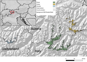
The Ötztal and Stubai ranges are neighbouring mountain regions in the Austrian state of Tyrol, bordering on Italy to the south and extending to the Inn valley in the north (Fig. 1). The Ötztal is home to 206 glaciers, covering ~115 km2 – a major part of Austria's glacierized area. In 2017/18, almost 90% of the glaciers in the Ötztal were smaller than 1 km2 (Table 1). This ratio is similar in the Stubai range, which is smaller overall and has 117 glaciers covering a total area of 38 km2. Compared to Ötztal and Stubai, glaciers in the Silvretta range are generally smaller and located at lower altitude. The mean elevation of glacier termini is ~2650 m a.s.l. in the Silvretta range, 2820 m a.s.l. in the Stubai range and 2860 m a.s.l. in the Ötztal range.

Fig. 1. Overview of the three study regions. Coloured glacier areas show the extent of the glaciers at the end of period 3 (2017/18).
Frequency distribution of elevation change
Our analysis is focused on glacier surface elevation change (dz). In particular, we extracted the frequency distribution of dz across the entire glacier area for each glacier in our data sets. Difference rasters for the respective time periods were cropped by the shapefile of the glacier boundary corresponding to the more recent DEM used to compute each difference raster. We chose to crop the rasters with the glacier boundaries corresponding to the end of each time period to exclude areas that became ice-free between the beginning (t1) and end (t2) of the time period. dz between t1 and t2 cannot be greater than the ice thickness at t1 in these areas. Accordingly, in cases where ice thickness was low at t1, dz values for areas that became ice-free between t1 and t2 can be low compared to other sections of the glacier with thicker ice, where dz represents the melt over the entire time period rather than just until the disappearance of the ice. Cropping with the t2 boundaries means that information on surface elevation change in the newly ice-free areas is lost, but avoids creating a bias towards low dz values in the dz frequency distribution patterns that would affect the further analysis. For each glacier, the distribution of values in the cropped difference raster was extracted in the manner of a histogram, using 0.05 m bins, and normalized by dividing by the glacier area corresponding to the respective dz bin. The result is a data set of one vector per glacier and time period, identifiable by the glacier's inventory ID number. These vectors were then used as input data for the SOM analysis, which we used to identify recurring patterns in the dz distributions.
The frequency distribution of dz represents key characteristics of the changes occurring at individual glaciers in a condensed manner: For an idealized glacier where surface elevation does not change in any part of the glacier, this distribution would resemble a line at dz = 0. In scenarios closer to the real world, a narrow distribution with a maximum at or near 0 indicates that elevation change is small for the majority of the glacier area (Fig. 2). Regardless of which dz value is most frequent, distribution curves in the shape of narrow spikes indicate that surface elevation is changing at a relatively uniform rate throughout the glacier area, while broader distributions with less pronounced frequency maxima suggest that surface elevation is changing with an irregular pattern, with greater rates of change in some parts of the glacier than in others.

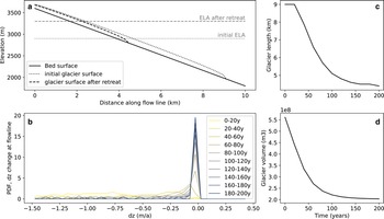
Fig. 2. Simple idealized glacier, Open Global Glacier Model (OGGM) run with linear mass-balance gradient. (a) 2D representation of the initial glacier surface, as well as the glacier surface after retreat to a new steady state after 195 years. (b) Probability density function of dz change along the flowline as plotted in (a), for 20-year time steps during the model run. The distribution curves are weighted by the widths of the glacier perpendicular to the flowline at each grid cell as an approximation of the area normalization carried out for the real-world frequency distribution examples. (c, d) Modelled glacier length and volume change corresponding to panels a and b.
We briefly consider what this looks like for the retreat of a simple test glacier constructed with the Open Global Glacier Model (OGGM) (Maussion and others, Reference Maussion2019). OGGM is a modular, numerical modelling framework for mountain glaciers and was chosen here due to its ease of use and generalized approach. The initial geometry of the test glacier is in steady state with a linear mass-balance gradient, extends from 3600 to 1980 m a.s.l., has an area of 4.5 km2 and a volume of 0.56 km3. The equilibrium line altitude (ELA) is at 2900 m a.s.l. The vertical extent was chosen to broadly approximate the LIA extent of glaciers in the Ötztal range (Charalampidis and others, Reference Charalampidis2018) and the ELA is based on values of transient ELA reported for Hintereisferner by Kerschner (Reference Kerschner1997) and environmental ELA around 1900 in our study region (Žebre and others, Reference Žebre2021). The term environmental ELA refers to the ‘regional altitude of zero glacier mass balance without the effects of shading, avalanching, snow drifting, glacier geometry or debris-cover’ (Anderson and others, Reference Anderson, Anderson, Armstrong, Rossi and Crump2018; Žebre and others, Reference Žebre2021). The simulation is not intended to exactly model the evolution of any particular glacier. Rather, the purpose of the model run is to illustrate the concept of the changes in dz distribution for a retreating glacier that reaches a new equilibrium in a simple, strongly idealized case.
The initial glacier state is perturbed by moving the ELA to 3300 m a.s.l., in order to simulate the glacier stabilizing at significantly reduced size. The new ELA value is within the range of expected environmental ELA for the year 2040 in our study region (Žebre and others, Reference Žebre2021). The modelled glacier reaches a new equilibrium after 195 years, having lost about 65% of its initial volume. The corresponding response time (Oerlemans, Reference Oerlemans1997) is 40 years, which is within the range of values for Alpine glaciers reported by Zekollari and others (Reference Zekollari, Huss and Farinotti2020). Figure 2 visualizes this scenario, as well as the dz distribution profiles along the modelled central flow line of the idealized glacier. Rates of loss remain relatively high until ~75 years into the simulation, when the decrease in length and volume markedly flattens off (2 c, d). During the phase of greatest disequilibrium at the beginning of the simulation, dz distributions are very broad. As the idealized glacier approaches its new steady state, loss rates flatten off and the dz distributions gradually shift to narrow profiles with each further time step.
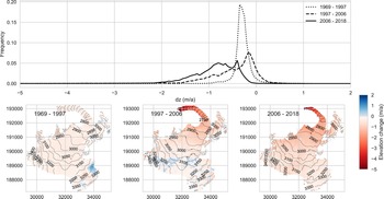
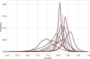
Figure 3 shows the dz frequency distribution at Gepatschferner, the largest glacier in the Ötztal, alongside maps of the corresponding elevation change to provide a real-world example. Ice flow velocity measurements at Gepatschferner during the last 10 years show that velocities have decreased at all elevations and were close to zero in the terminus region in the most recent years, while the slowdown is less pronounced in the upper regions (Stocker-Waldhuber and others, Reference Stocker-Waldhuber, Fischer, Helfricht and Kuhn2019).

Fig. 3. Frequency distribution curves of dz at Gepatschferner for three different time periods (top panel). The maps in the bottom panel show the corresponding spatial distribution of dz.
SOM-analysis
An SOM is a comparatively simple type of unsupervised machine learning algorithm that is commonly used to visualize and/or identify patterns or clusters in complex data sets based on dimensionality reduction. The SOM places nodes on a grid in the input data space (here, the input data are the dz frequency distribution profiles of all glaciers in our data set), with a weight vector of the same dimension as the input vectors assigned to each node. The winning node, or best-matching unit (bmu), and neighbouring nodes within a particular distance are determined for each input vector (here: each dz frequency distribution profile). The winning node as well as neighbouring nodes are updated in each training iteration to better represent the input data. The SOM preserves the topology of the input data it is trained on and the nodes of the trained SOM represent a classification of the input data into discrete clusters. The nodes are distributed in the SOM space to represent the distribution of the input data, i.e. more nodes are placed in areas with more input samples, while nodes are scarcer where there are fewer input samples (Kohonen, Reference Kohonen2001). In our case, the result of the SOM analysis is a certain number of winning nodes and weight vectors that each represent a subset of the input data, i.e. the SOM generates representative types of dz profiles from the input data and each input dz profile is grouped to one of these types.
We refer to the publications of Kohonen (Reference Kohonen1990, Reference Kohonen1991, Reference Kohonen2001, Reference Kohonen2012), who developed the SOM technique, for detailed background on the principles of the SOM algorithm. SOM are applied across a broad topical spectrum, including meteorology and climate science, and throughout the geosciences, often in the context of automated classifications of remote-sensing data. Glaciology-specific uses of SOM are relatively rare to date, but include, e.g. automatic crevasse detection from LiDAR DEMs (Foroutan and others, Reference Foroutan, Marshall and Menounos2019). Further exemplary case studies and summary reviews can be found in Hewitson and Crane (Reference Hewitson and Crane2002), Agarwal and Skupin (Reference Agarwal and Skupin2008), Liu and Weisberg (Reference Liu and Weisberg2011) and Sheridan and Lee (Reference Sheridan and Lee2011). Clustering glaciers into groups to show recurring types of responses and variations therein has many potential uses, particularly in the context of assessing regional pattern variability (e.g. Moon and others, Reference Moon2014), and we suggest that using an SOM approach to automate the clustering procedure is an efficient work flow that can be tuned for different data sets and types of analyses. We implement the SOM algorithm using the opensource MiniSom package (Vettigli, Reference Vettigli2018) for python.
In our analysis, the number of nodes in the SOM (also referred to as the size of the SOM) corresponds to the number of types of dz profiles that are used for clustering the input data. The size of the SOM as well as the number of training iterations and parameters of the learning and neighbourhood functions can be tuned: A larger SOM will result in a finer resolution of different types, while a smaller SOM groups the input data more broadly. Whether a larger or smaller SOM is better suited to meaningfully identify clusters depends on the nature of the input data and the application. While larger SOM result in a finer resolution of types, the types eventually become so similar to one another that they are no longer useful for further interpretation in the context of identifying common patterns of glacial melt on a regional scale. Smaller SOM inherently tend to group rarer ‘extreme’ types, i.e. very flat or very spiky distribution curves, into clusters where their characteristics are averaged out to a large degree, so that potentially interesting information is lost. This is equally undesirable for further interpretation from a glaciological point of view.
Like the size of the SOM, the initial values for the learning rate and the neighbourhood function can be seen as tuning parameters that affect the final outcome. Appropriate values depend on the nature of the data and the application and are commonly determined by trial and error and comparing average quantization errors (QE) of different setups (Schuenemann and others, Reference Schuenemann, Cassano and Finnis2009; Sheridan and Lee, Reference Sheridan and Lee2011; Foroutan and others, Reference Foroutan, Marshall and Menounos2019). Here, the goal of the SOM analysis is to generate representative types of dz profiles that are interpretable in the context of glacier imbalance, as illustrated in Figure 2. We chose our initial values based on two criteria: (1) whether the winning nodes (types) are realistic, meaningful generalizations of dz profiles found in our data sets and (2) QE as a measure of statistical representativity. QE is computed as the Euclidean distance between the input vectors and the nodes they are assigned to. The average QE of the SOM can be seen as a measure of how well the SOM nodes represent the data overall, while the QE of individual input vectors is a measure of how well that particular vector is represented by its assigned node.
We aim for a broad generalization of dz patterns and find that a relatively small SOM-size of 3×3 nodes suits this purpose, forming a compromise between obtaining clearly distinguishable distribution types and representing the entirety of the distribution spectrum. A smaller SOM-size of 2×3 nodes produces similar outcomes for dz distributions with positive and moderately negative frequency maxima but fails to resolve differences in distributions with very negative frequency maxima, which we want to preserve for our analysis. With SOM-sizes of 4×3 nodes or larger, extra nodes are added in the region of the data space that contains the most input data (Supplementary Fig. 1). This means that the extra nodes are relatively similar to each other. Like this, differences are resolved more finely for the most common types of distributions but do not add much new information, whereas the representation of the more rare distribution types remains mostly unchanged. We consider anything larger than a 3×3 SOM to be beyond the ‘elbow criterion’ (e.g. Schuenemann and others, Reference Schuenemann, Cassano and Finnis2009) above which the added information is no longer useful for our particular analysis.
We use a value of 0.5 for the initial spread of the neighbourhood function as well as for the initial learning rate. The initial spread of the neighbourhood function determines the distance in which the SOM looks for the best-matching unit (bmu) that is assigned to the input vectors, while the initial learning rate determines the degree to which the bmu and neighbouring nodes are adjusted to approach the input data they are matched with in the first iteration. Both the spread of the neighbourhood function and the learning rate decrease with time. High values for the initial spread of the neighbourhood function result in very similar winning weight vectors, whereas very low values produce unstable results. Within the range of values that produce what we consider to be realistic dz distribution types, we select the value with the lowest average QE. A high initial learning rate leads to a large impact of individual dz profiles on the shape of the winning weight vectors and high overall QE, while a very low initial learning rate leads to lower QE but does not resolve the differences in the winning types that we wish to preserve (Supplementary Fig. 2).
The SOM nodes are initialized using the first two principal components (Jolliffe, Reference Jolliffe2011) of the training data and the SOM is trained sequentially. This ensures that the output is exactly reproducible and does not depend on random processes as it would with random initialization and training sequencing (Akinduko and others, Reference Akinduko, Mirkes and Gorban2016). We consider this beneficial for our specific application since it allows us to better compare the SOM weight vectors resulting from different configurations. We train the SOM in 4000 iterations – average QE does not noticeably decrease beyond this value for our setup.
We train the SOM on dz distributions from the Ötztal Alps. The Ötztal is one of the most extensively glacierized parts of the Austrian Alps and glaciers of all size classes occurring in Austria can be found here, across a relatively broad range of elevations. Accordingly, any common patterns of dz distribution to be found for glaciers in western Austria are likely to be represented in the Ötztal data set. We use the entire Ötztal data set – a total of 604 dz distribution vectors, 196 for the period 1969–1997, 205 for the period 1997–2006 and 202 for the period 2006–2017/18 – to generate the SOM. In a further step of the analysis, the trained SOM is applied to other regional data sets to compare patterns in dz distributions across different mountain ranges.
Results
SOM generation and node characteristics
Figure 4 shows the normalized frequency distribution of dz for all of the glaciers in the Ötztal data set split into the three time periods. The figure is intended to provide a general overview of the dz distributions present in the data set. While all three periods show a range of different distribution types, there are noticeable differences between the periods that can be generalized as follows: From 1969 to 1997 (period 1), most glaciers showed a decrease in surface elevation in most of their area and the frequency maximum is at a negative dz value. However, positive surface elevation change in some areas was also recorded for many glaciers, i.e. the distribution curves extend into positive dz values. For 1997–2006 (period 2), the most noticeable difference to the previous period is that the majority of curves have become ‘flatter’, i.e. the range of dz values that occur at the respective glaciers has increased. Many glaciers still record some positive elevation change, but there are more areas with increasingly negative dz values. In the most recent period, 2006–2017/18 (period 3), fewer glaciers than in previous periods show any positive change, and those that do show only small increases in small parts of their area. For most glaciers, distribution curves remain comparatively flat with a large range that extends increasingly into more negative values. However, some glaciers shift to more ‘spiky’ distributions with very pronounced frequency maxima, mostly at values just below 0. There are two core characteristics that are likely to define any clustering scheme that groups individual distribution curves into types: The dz range or shape of the curve (‘flat’ vs ‘spiky’), and the magnitude of the most frequent dz value.
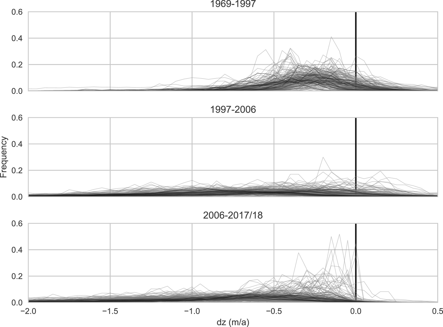
Fig. 4. Frequency distribution of surface elevation change (dz) for all glaciers in the Ötztal data set, grouped by the three available time periods. Black lines represent glaciers that were larger than 1 km2 at the end of each time period, grey lines represent glaciers smaller than 1 km2.
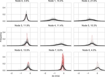
We use all three time periods and all glaciers in Ötztal to train the SOM to ensure that the variability of dz distributions seen over the three time periods is represented in the SOM-based type classification. In Figure 5, the nine weight vectors of the 3×3 SOM are shown in one plot to facilitate a direct comparison of the distribution types the SOM identifies and which will be discussed further in the following sections. Generalizing very broadly, there are two very narrow (spiky) distribution types with differing values of maximum frequency dz (nodes 0 and 7), and three very broad (flat) distribution types, similarly with differing values of maximum frequency (nodes 1, 2 and 4). Additionally, there are four ‘transition’ types, two of which are on the narrower side (3, 6) and two that are broader (5, 8). Only node 8 – one of the transition types – has its frequency maximum at a value slightly above 0 and shows roughly the same amount of positive as negative elevation change. In terms of frequency maxima, nodes 8, 7 and 6 (in that order) are the most ‘balanced’ nodes in the sense that for the associated glaciers, most grid points show dz change relatively close to 0 ma1. Nodes 0, 3 and 4 have more negative frequency maxima, i.e. are more imbalanced. The most negative frequency maxima occur in nodes 1, 2 and 5. See Table 2 for a summary of the most frequent dz values and the approximate range of each type (or: SOM weight vector).
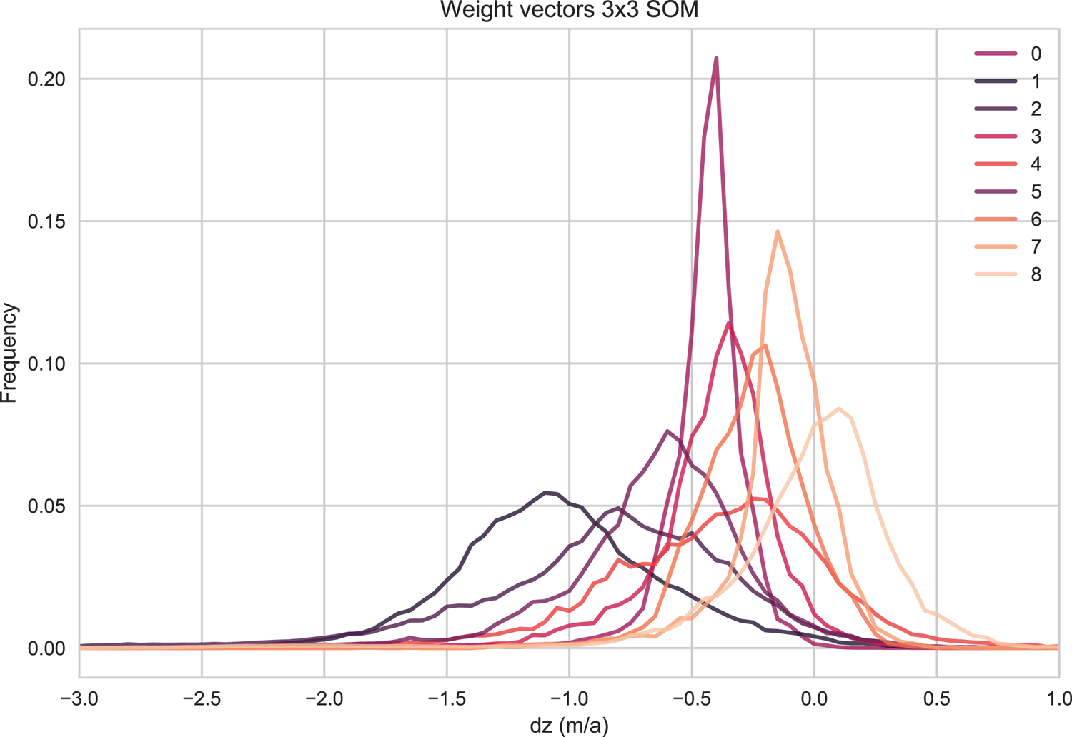
Fig. 5. Weight vectors of the SOM nodes. Each weight vector can be thought of as a representative of a generalized pattern of dz frequency distribution that occurs in the surface elevation changes of all glaciers in the Ötztal Alps between 1969 and 1997, 1997 and 2006, and 2006 and 2017/18.
Table 2. Summary characteristics of the winning weight vectors of each SOM node, corresponding to Figure 5

Range is given as the range of dz with frequency values >0.01.
In Figure 6, the weight vectors are displayed in subplots corresponding to their assigned node position in the SOM space and plotted over all input vectors mapped to the same node. In total, 21.6% of the input data are mapped to node 2. Nodes 1, 3, 4, 5 and 6 each represent between 10 and 14% of the input data. The ‘rarest’ distribution types are grouped in node 7 (8.8%) and nodes 0 and 8 (both about 4%).
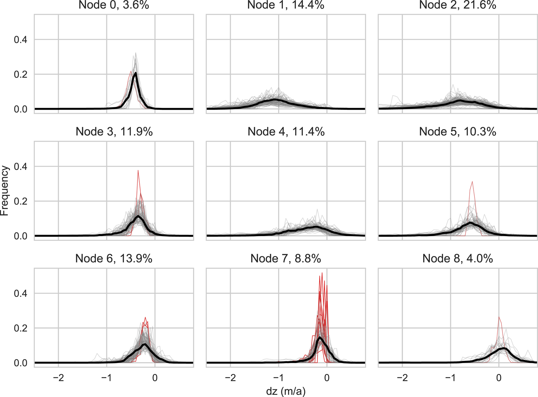
Fig. 6. SOM nodes with weight vectors (same as in Fig. 5) plotted at their locations in the SOM space. Bold black lines denote the weight vectors, thin grey lines the input vectors mapped to each node. Percentage values in the plot titles give the percent of input data mapped to each node. Red lines represent the input vectors with the highest quantization errors (3% of total input data).
QE for all individual input vectors, i.e. the distance between the input vectors and their corresponding SOM weight vector, are computed to assess how well each input vector is represented by its assigned node. The range of individual QE values is mostly between 0.05 and 0.15 (Supplementary Fig. 3). Higher QE values occur primarily in nodes 6 and 7 for input vectors with very narrow frequency distributions. The 3% of input data with the highest individual QE values are highlighted in red in Figure 6 to illustrate what relatively poor representation of input dz profiles by the SOM nodes looks like, compared to better matches (grey lines). Of the 19 input vectors with high QE shown in Figure 6, 11 occur in node 7, three in node 6, two in node 3, and one each in nodes 0, 5 and 8. Since the input vectors are tied to a glacier ID number, the glaciers with distributions with high QE can be viewed individually. Only the three largest exceed 0.05 km2 in size and none are larger than 0.07 km2. The small size and limited altitudinal range of these glaciers leaves little room for variations in altitude or geometry that could cause variations in dz, hence the narrow frequency distributions. In terms of SOM quality, the conclusion that can be drawn here is that the SOM poorly represents the narrowest of the frequency distributions, which occur at a small number of ‘very, very small’ glaciers.
Applying the trained SOM to neighbouring mountain ranges of Stubai and Silvretta yields QE of similar magnitudes as for the training data (Ötztal). The magnitude of the most frequent errors is similar for Ötztal and Stubai, and slightly higher for the Silvretta range. Large errors are rare and tend to be associated with narrow distribution curves at small and very small glaciers, like in the Ötztal training data set. Overall, this suggests that the patterns identified in the Ötztal data set reasonably represent those found in the other regions and that there are no substantially different patterns in the other regions that are not contained in the training data.
To provide a better sense of how the dz frequency distribution curves ‘translate’ into more traditional representations of surface elevation change, Figure 7 shows the median dz value per 20 m elevation bands for each glacier in the three regions, arranged by their assigned SOM nodes analogous to Figure 6 and colour coded by time periods. Glaciers clustered into the very broad and negative nodes 1 and 2, which occur mostly in the latter two time periods, tend to show dz-elevation profiles with the most negative values at lower elevations. The rate of dz change decreases with increasing elevation but does not reach zero for most of these glaciers. Elevation has a very strong influence on dz for the glaciers grouped into the broad, ‘flat’ nodes (1, 2, 4). The influence of elevation on dz and the rate of change of dz is less pronounced for profiles mapped to nodes representing narrower dz distribution curves (nodes 0, 3, 6 and 7). With the exception of the narrowest nodes (0, 7), dz is typically more negative at lower elevations for narrow and transitional distributions, but dz elevation profiles reach elevations above which dz remains largely constant. The patterns associated with the nodes are comparable across the three regions, with nodes 1 and 2 showing strong elevation dependency and negative dz at lower elevations. There are fewer glaciers in the Silvretta range than in the other two regions and these glaciers have a relatively small altitudinal range. Not all of the SOM nodes are found in the Silvretta range (no Silvretta glacier was grouped to node 8), which reflects the lower overall variability of types of glacier response in this region compared to the Ötztal and Stubai ranges.
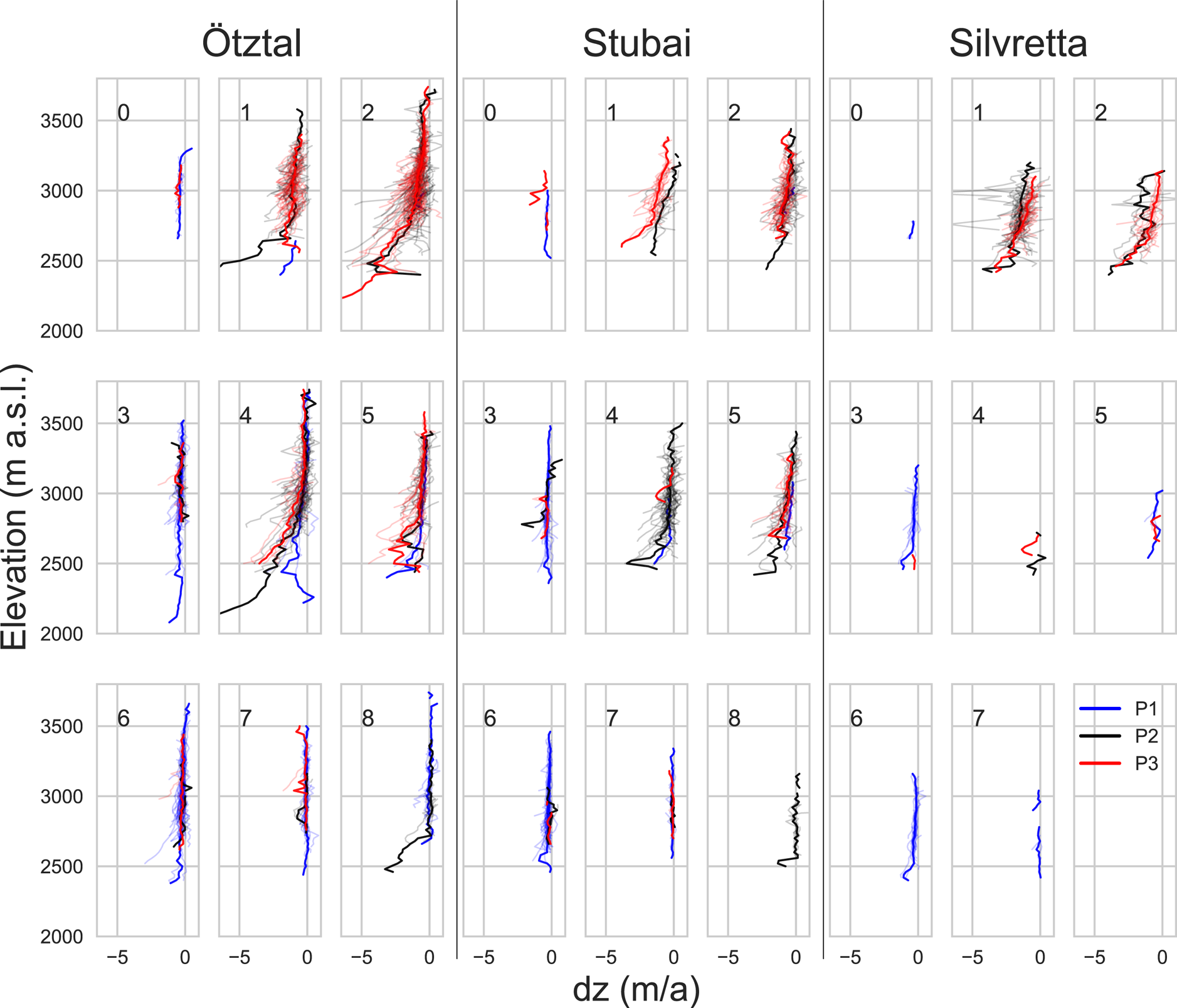
Fig. 7. Median surface elevation change per 20 m elevation bands for the three regions. Blue lines represent time period 1 (1969–1997; years given in parentheses are for the Ötztal and Stubai region, see Table 1 for DEM acquisition years in the Silvretta region), black lines represent time period 2 (1997–2006), and red lines represent time period 3 (2006–2017/18). The grouping in subplots is analogous to the nodes in Figure 6, node numbers are noted in the respective subplots. Thin lines represent individual glaciers, the bold lines represent the median values of all glaciers per SOM node and time period.
Pattern changes over time
Splitting the data into the three different time periods allows for a quantification of the shift in dz distribution types that can qualitatively be seen in Figure 4: In period 1 (1969–1997), most input data is mapped to narrow transition types (for Ötztal: node 3: 24%; node 6: 32%; Table 3, Fig. 8). In period 2 (1997–2006), nodes 2 (32%), 4 (22%) and 1 (19%) are most common – these are the ‘flattest’ distribution types. In period 3 (2006–2017/18), nodes 1 and 2, the most negative of the flat distributions, dominate at 23 and 32%, respectively. Compared to period 2, there is a slight increase of input vectors that are mapped to nodes with a narrower range, specifically nodes 0, 3, 6 and 7.
Table 3. Percentage of total input data mapped to each node per time period and region
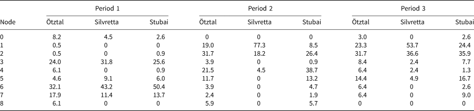
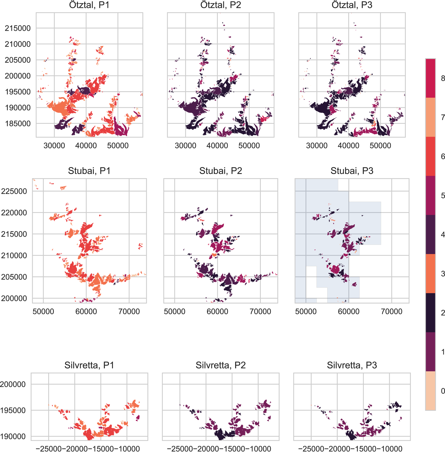
Fig. 8. Glacier extent in the three ranges at the end of periods 1, 2, and 3, with individual glaciers coloured to indicate the SOM node they are mapped to in each period. Colours match the colour scheme in Figure 9 and Figure 5. Note that for Stubai, some glaciers in the eastern half of the range are missing in P3 because they were not covered in the geodetic surveys of 2017/18. The grey shading indicates the smaller extent of the 2017/18 DEM in the Stubai region. Coordinates in meters. CRS: EPSG 31254 (MGI Austria GK West).
For most glaciers in the Ötztal, the shift to very negative, broad dz distribution patterns occurred between periods 1 and 2, with a minor fraction of glaciers shifting back to narrower patterns in period 3. This overall trend is the same in the other two regions – most glaciers shift to nodes 1, 2 and 4 between periods 1 and 2. This shift is practically total in the Silvretta range and less immediate in the Stubai and Ötztal ranges. In the Silvretta range, no glacier is mapped to the ‘flat’ nodes (1, 2, 4) in period 1. In period 2, 77% are mapped to the most negative, flat distribution type (node 1). In the Stubai range, nodes 3 and 6 (narrower transition types) are dominant in period 1, like in the Ötztal range. In period 2, the majority of glaciers are mapped to the very broad nodes (2 and 4). In period 3, nodes 1 (broad, very negative) and 2 become dominant and fewer glaciers are mapped to the less negative node 4. Like in Ötztal, there is an increase in glaciers mapped to narrow distributions (nodes 0, 3 and 7) for period 3 compared to period 2. This shift to narrow distributions is absent in the Silvretta range (Table 3, Fig. 8). In all three regions, all larger glaciers, including the size class between 0.5 and 1 km2, are mapped to one of the broader nodes (1, 2, 4, 5) in period 3 (Supplementary Fig. 4). All glaciers that are in narrower nodes (0, 3, 6, 7) in period 3 are very small. No glaciers are mapped to node 8 in period 3 (positive frequency maximum, most ‘balanced’ type).
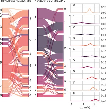
By tracing which node individual glaciers are mapped to in each of the three time periods, shifting melt patterns can be visualized on a regional scale (Figs 8, 9). As mentioned above, in period 1 most glaciers are mapped to nodes 3, 6 and 7 – patterns with a similar, moderate spread of dz values. Node 3 has a more negative frequency maximum than nodes 6 and 7, which exhibit noticeable positive surface elevation change on the right tail of the distribution. The majority of glaciers mapped to nodes 3 and 6 in period 1 shift to very broad nodes (1, 2 and 4) in period 2 (Fig. 9). In general, few glaciers remain in the same node between period 1 and 2. There is a clear tendency for glaciers to shift from narrow distributions to broader ones within the observed periods, besides the expected shift to increasingly negative frequency maxima. Most glaciers mapped to nodes 1 and 2 in period 2 remain there until period 3, or move from 1 to 2 or vice versa. Transitions from these very broad distributions back into narrower types are comparatively rare, although some shifts from broad distributions into very narrow ones do occur, as discussed previously. Some of the glaciers mapped to the least negative of the broad distributions (node 4) in period 2 shift to the less flat and more negative node 5 in period 3. In Figure 8, it is evident that a large majority of glaciers and particularly the larger glaciers in all regions have shifted to ‘flat’, strongly negative dz distribution patterns.

Fig. 9. Overview of how surface elevation patterns of individual glaciers in all three regions changed throughout the three time periods. Colours represent the nodes/weight vectors as shown on the right. The width of the coloured swaths is proportionate to the number of input vectors mapped to each node. The left side of the Sankey plot represents the 1969–1996 period, the middle the 1997–2006 period and the right side the 2006–2017/18 period.
Discussion
Input data and SOM algorithm
The SOM algorithm we apply in this study facilitates the clustering of a relatively large data set that would otherwise be challenging to objectively divide into discrete classes in a statistically meaningful way. However, like all machine learning approaches and statistical modelling, the quality of the classification depends strongly on the quality of the input data. The topographic information available for the individual glaciers and time periods is subject to uncertainties stemming from the nature of the respective DEMs. As referenced in the section on the geospatial data, various publications have detailed the Austrian GI and underlying data and have (1) quantified uncertainty and (2) established that surface elevation change over glacier areas is generally large compared to DEM uncertainties in our study region. Nonetheless, vertical uncertainty associated with the DEMs is clearly relevant to any analysis of surface elevation changes. Rather than quantifying absolute volume change in the region or at single glaciers, our study focusses on identifying recurring dz distribution patterns and how these patterns shift over time. To assess whether the DEM uncertainties are potentially large enough to significantly change either the identified patterns or their evolution in time, we proceed as follows: For each of the three difference rasters from the Ötztal region, we add a random number within the respective assumed accuracy range to each pixel. We then repeat our analysis, training the SOM on these data with otherwise unchanged initial conditions. The assumed uncertainties are ±2.7 m for period 1 (Eder and others, Reference Eder, Würländer and Rentsch2000), ±0.8 m for period 2 (Abermann and others, Reference Abermann, Fischer, Lambrecht and Geist2010a) and ±0.3 m for period 3 (see section on geospatial data and: Abermann and others (Reference Abermann, Fischer, Lambrecht and Geist2010a), Fischer and others (Reference Fischer, Seiser, Helfricht and Stocker-Waldhuber2021)).
Sailer and others (Reference Sailer, Rutzinger, Rieg and Wichmann2014) quantified the accuracy of surface elevation change calculations based on LiDAR DEM difference rasters for a number of geomorphic processes, showing that errors increase for steep slopes and high surface roughness, as well as low point densities. Glaciers in our study area are rarely steeper than the 40° threshold above which errors increase markedly (Sailer and others, Reference Sailer, Rutzinger, Rieg and Wichmann2014) and the ice surface is mostly smooth compared to the surrounding areas, so that large pixel-wise variability in uncertainties seems unlikely at the scale of individual glaciers, at least for the latter two time periods. The addition of random noise introduces more variability for individual glaciers’ dz distribution pattern than we expect based on the above and we consider our approach for the error estimation relatively conservative. Our analysis is based on the distributions of pixel-wise dz and does not involve spatial averaging of absolute or relative dz change. Hence, we consider potential variability of dz uncertainty within individual glacier boundaries the most relevant factor that may affect the outcome of the analysis and disregard spatial correlation of errors as discussed in, e.g. Rolstad and others (Reference Rolstad, Haug and Denby2009) and Fischer and others (Reference Fischer, Huss and Hoelzle2015c), acknowledging that this is a considerable simplification.
Figure 10 shows the winning weight vectors of the SOM for the original input data as discussed previously alongside the winning weight vectors of the SOM trained on the modified input data. Qualitatively, the distribution of nodes is similar, with a range of broad, transitional and narrower distribution types. Quantitatively, the broadest nodes (1, 2, 4) are very similar in both versions, as are the narrow nodes (0, 7) and the single node with a positive dz frequency maximum (8). Lager differences in the range and the placement of the frequency maxima occur for the transitional nodes (3, 5, 6). Input vectors from the three time periods shift between nodes in the same way for the original and the modified data, i.e. the majority of glaciers shift from narrower to very broad patterns, with a small number reverting to narrow, negative patterns from broader ones. Table 4 shows the differences in the amount of input data mapped to each node for the three time periods to quantify how pattern changes over time differ between the original and modified input data. The highest absolute differences occur in period 1 for nodes 5 and 6, with −10.6 and +12.8%, respectively. For all other time periods and nodes, differences are considerably lower. Nodes 5 and 6 represent transitional patterns, which are more similar to each other than the ‘extreme’ nodes that represent either very broad or very narrow distributions. Added noise in the input data is more likely to cause shifts between similar nodes than shifts between nodes representing very different distribution types. Accordingly, having the largest differences for these transitional patterns is to be expected. Considering the overall very similar nature of the winning weight vectors for the original and modified data sets and the preservation of pattern shifts over time, we consider the shape of the distribution curves robust enough to the inherent vertical uncertainty of the DEMs to allow for the presented clustering analysis.

Fig. 10. Winning weight vectors for the original input data in black (same as Fig. 5), and winning weight vectors for input data modified to estimate the potential influence of DEM uncertainties in red.
Table 4. Difference between percentage of Ötztal input data mapped to each node in each time period when comparing original input data and data modified with random noise within the accuracy estimates for the DEM difference rasters
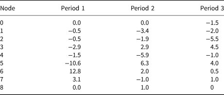
Positive values mean that more values were mapped to a node when using the original input data, negative values mean more values were mapped to a node when using the modified input data.
The source data for the photogrammetric as well as the LiDAR data was collected around the time of minimum seasonal snow cover, so that potential biases due to remnant snow are minimized. Nonetheless, snow cover and discrepancies in the mapping of glacier boundaries from one period to the next can cause significant errors. The time periods assessed in this study are dictated by the availability of DEM data and GI and hence vary in length. The characteristics of the dz distribution curves differ depending on the length of the time period used to compute the difference rasters and, accordingly, short-term variations cannot be resolved if the time interval between consecutive DEMs is too long. Period 1 covers roughly 30 years, while periods 2 and 3 each cover about 10 years with some variation between regions (Table I). Period 1 includes a phase in the late 1970s and early 1980s in which many glaciers in the study area showed a more or less balanced mass budget – some advanced slightly – while the more recent periods are dominated by recession (Abermann and others, Reference Abermann, Lambrecht, Fischer and Kuhn2009, Reference Abermann2010b; Fischer and others, Reference Fischer, Seiser, Waldhuber, Mitterer and Abermann2015b; Charalampidis and others, Reference Charalampidis2018; Fischer and others, Reference Fischer, Seiser, Helfricht and Stocker-Waldhuber2021).
In the SOM classification, single glaciers with erroneous distribution curves can strongly affect the characteristics of the nodes, since they can expand the input data space. In the Ötztal data set, three glaciers showed very atypical distributions, which were found to be the result of inconsistent mapping of glacier boundaries from one time period to the next (regions identified as part of the glacier in one period were not identified as such in the following period, or vice versa). The respective dz distribution curves were removed from the data set prior to the SOM classification. Not removing them results in an SOM with a markedly different distribution and an ‘artificial’ node placed in the space of these outliers. While the SOM algorithm is undoubtedly a powerful clustering tool, this highlights the need for cautious quality control of the input data and interpretation of results, as well as an in-depth understanding of the underlying input data.
Aside from the input data, the main factors that affect the results of the SOM classification are the size of the SOM, the number of iterations, the learning rate and the decay function. Changing any of these will result in changes to the weight vectors and node placements, although the overall patterns identified in the SOM remain the same within a reasonable range of values for the input parameters (Supplementary Fig. 1 shows the nodes for different SOM-sizes, Supplementary Fig. 2 shows the effect of changing the initial learning rate and neighbourhood function). For the purpose presented in this study, the primary measure of whether the SOM classification is useful is whether the identified types (weight vectors) make sense as a representation of different glacier states, combined with a low overall QE as an indicator of statistical soundness. The former is – to some degree – subjective and hence inherently debatable. The SOM nodes used to classify the glaciers in this study are not meant as a definitive, universal glacier typology. Rather, they serve for an overview analysis at a regional scale, showing common patterns as well as allowing for the identification of sub-regions or individual glaciers that do not follow these patterns.
Interpretation of results
In terms of glacier state, node 1 represents glaciers that are rapidly losing mass over their entire area and are far out of balance (Fig. 5). Nodes 2 and 4 have a similarly broad distribution without very pronounced frequency maxima but are less negative than node 1. Once grouped into nodes 1 or 2, the glaciers in our data sets tend to stay there until the end of our study period. A small number of glaciers grouped to broad nodes in period 2 shift to narrower nodes (0, 3, 7) in period 3 (Fig. 9). This is typically the case for very small glaciers where glacier area has become so small that factors governing local surface elevation change – such as aspect or elevation – do not vary significantly across the area of the glacier.
A closer look at the glaciers that shift into the narrowest nodes (0, 7) from broader nodes in period 3 reveals that their termini are at higher elevations than for glaciers in the other nodes, at least in the Ötztal range. This distinction is less clear in the Stubai range, where there are fewer glaciers overall and fewer glaciers in the respective nodes. All of the glaciers grouped into nodes 0, 3, 6 and 7 in period 3 are very small (maximum size: 0.4 km2), but not all very small glaciers shift back to narrow nodes in period 3. We suggest that glaciers that shifted from broader nodes (1, 2, 3, 4, 5, 6) to node 7 (narrow, not very negative) in period 3 have significantly reduced their imbalance by retreating. They all show less surface elevation loss in period 3 than in period 2 (mean values: −0.5 m a−1 for period 2 vs −0.1 m a−1 for period 3), while loss rates have increased at glaciers that shifted into node 7 from the ‘positive’ node 8. Glaciers that shift from broader nodes to node 0 have similarly narrow distribution profiles but at more negative frequency maxima, so that rates of loss are becoming more uniform across the glacier area but are not necessarily decreasing overall.
We consider nodes 3, 6 and 7, common in period 1, to represent glaciers that are losing mass but have significant ice flow from upper to lower elevations that still partially compensates for increased melt at lower elevations. This also reflects the 1980s glacier advance in the study region (Abermann and others, Reference Abermann, Lambrecht, Fischer and Kuhn2009; Fischer and others, Reference Fischer, Seiser, Waldhuber, Mitterer and Abermann2015b). Excluding the very small glaciers that shift back into narrow nodes in period 3, glaciers with pronounced frequency maxima are assumed to have a comparatively large dynamic component affecting the evolution of surface elevation, in addition to topographic or geometric factors. Conversely, the very broad distribution of nodes 1, 2 and 4 indicates that the decrease in surface elevation occurs at highly variable rates across the glacier area, which suggests a reduced dynamic component and lack of ice transport to the termini. It follows that factors such as aspect, slope and elevation are the main drivers of local melt rates in the lower sections of these glaciers.
The widespread shift to broad negative dz distributions is indicative of rapid glacier recession and reduced ice flow, which is in line with findings from case studies based on long-term in situ measurements of ice flow and mass balance in the Ötztal Alps and other regions of the world: Stocker-Waldhuber and others (Reference Stocker-Waldhuber, Fischer, Helfricht and Kuhn2019) report decreasing ice velocities at measurement stakes at the Ötztal glaciers Kesselwandferner and Hintereisferner in recent decades, with shorter time series from neighbouring Gepatsch- and Taschachferner showing the same signal, and interpret this as a ‘strong sign’ of severe glacier recession. At Mer de Glace in the French Alps, it is estimated that two-thirds of an observed increase in thinning is due to reduced ice flux, while one-third is thought to be due to increased surface ablation (Berthier and Vincent, Reference Berthier and Vincent2012). In the Himalayas, decreasing ice flow velocities and fluxes tied to increasing glacier imbalance have been observed at individual glaciers (Azam and others, Reference Azam2012; Sugiyama and others, Reference Sugiyama, Fukui, Fujita, Tone and Yamaguchi2013), as well as on a regional scale (Dehecq and others, Reference Dehecq2018). We suggest that dependencies between dynamic regime, velocity and – by extension – surface elevation change can be grouped into meaningful patterns for glaciers with distinct characteristics, and that such classifications are useful for identifying regional patterns and trends for further analysis.
States of disequilibrium
Several recent studies address the disequilibrium of small mountain glaciers. Christian and others (Reference Christian, Koutnik and Roe2018) laid out how glacier response time controls the evolution of disequilibrium, showing the applicability of these concepts across a wide range of glacier geometries. Zekollari and others (Reference Zekollari, Huss and Farinotti2020) assessed the response times and committed loss, i.e. the amount of ice that would be lost before a new balanced state is reached if the climate were to remain constant, of glaciers in the Alps by forcing a dynamical model with the surface mass balance of the previous 30 years, for each year between 2001 and 2018. They found higher relative committed loss for smaller glaciers and show that committed loss increased in the early 2000s and stabilized after 2010. Using the temperature forcing required to retain the glacier volume of a given year as a further measure of imbalance, they again showed that imbalance decreased after 2010 compared to the previous decade. They attributed the decrease in imbalance to geometric glacier change, i.e. fast retreat leading to a less pronounced state of imbalance. For the case of Vadret da Morteratsch (Switzerland), Christian and others (Reference Christian, Koutnik and Roe2018) showed that the climate-geometry imbalance was never larger than at the time of publication of the study, which suggests that glacier retreat has not begun to ‘catch up’ with climate forcing at this glacier. Pelto (Reference Pelto2006) found continued regional disequilibrium in the North Cascades (USA) for a study period up to 2002. Charalampidis and others (Reference Charalampidis2018) carried out a kind of committed loss study for three well-studied Austrian glaciers with long-term mass-balance time series: Hintereisferner, a relatively large valley glacier; Kesselwandferner, a smaller, steeper glacier; and Vernagtferner, which surged in the past. All three are in close spatial proximity. The authors found that Hintereisferner is the furthest from steady state, with inevitable and substantial further retreat. In contrast, Kesselwandferner would reach steady state faster, assuming a stable 1981–2020 climate. While Hintereisferner and Kesselwandferner can reduce imbalance by retreating, Vernagtferner primarily loses mass by thinning rather than area loss, so that imbalance is not reduced in the same way (Charalampidis and others, Reference Charalampidis2018).
From assessing the simple idealized glacier in Figure 2, we see a gradual transition from broad distribution patterns with strongly negative frequency maxima during the period of maximum disequilibrium, to narrower distributions with less negative frequency maxima as the glacier tends towards a new steady state. Comparing this with the SOM analysis, we suggest that the dominance of the very broad, negative distributions associated with nodes 1 and 2 implies that the majority of the glaciers in our data set are – unsurprisingly – far from steady state. The few glaciers that have shifted back into narrow distribution patterns with frequency maxima close to zero could be considered closer to a balanced state in a general sense. However, the linear mass-balance model and extremely simplified geometry of the idealized glacier clearly have limitations here. The underlying processes driving the shift to narrower patterns and associated reduced loss rates at these very small glaciers might be related to a range of factors, such as, e.g. geometric changes, accumulation due to local wind deposition patterns or regular avalanching gaining in relative importance as the glacier area shrinks, or reduced overall ablation due to loss of more sun-exposed sections of the glaciers (DeBeer and Sharp, Reference DeBeer and Sharp2009; Capt and others, Reference Capt, Bosson, Fischer, Micheletti and Lambiel2016; Huss and Fischer, Reference Huss and Fischer2016; Florentine and others, Reference Florentine, Harper and Fagre2020).
The three glaciers discussed by Charalampidis and others (Reference Charalampidis2018) are also contained in our data set for Ötztal: Hintereisferner shifts from node 4 (broad distribution with moderately negative frequency maximum) to node 2 (broad distribution, notably more negative frequency maximum) between periods 1 and 2 and remains there in period 3. Kesselwandferner shows a more varied response, moving from node 6 (transition type with moderate range) to node 4 (broader distribution with similar frequency maximum as node 6) and then to node 5 (more negative frequency maximum than nodes 4 and 6, shape of distribution between nodes 4 and 6) over the three periods. Vernagtferner moves from node 6 (transition type) to node 2 (broad distribution, very negative frequency maximum) and remains there. Due to the different methods and focus areas, a direct comparison is difficult, but overall we consider our results for the three glaciers in line with the findings of Charalampidis and others (Reference Charalampidis2018): Hintereisferner is far out of balance and has been for several decades. At Kesselwandferner, patterns are shifting more rapidly between nodes with slightly less negative frequency maxima than at Hintereisferner. Vernagtferner, which started in the same node as Kesselwandferner in period 1, shifted into a very imbalanced node in period 2 and remains there. These three glaciers can serve as an example of the compromise between generalizability and resolution that must be made in some way when comparing local and regional scales. As their case study has a very local focus and higher temporal resolution, Charalampidis and others (Reference Charalampidis2018) see differences in their responses that our SOM analysis only hints at. A larger SOM with more nodes would differentiate between glacier types in more detail – a SOM with as many nodes as glaciers would represent each dz distribution pattern exactly –, but would arguably hamper the regional overview. An interesting option for further studies especially with larger data sets would be to use a large SOM to generate a larger number of types and then carry out another level of grouping of the types, e.g. into broad, narrow and transitional patterns. This would allow for a more finely resolved analysis of differences between the most common types of patterns.
Determining how far a particular glacier is from its theoretical equilibrium at a given point in time is a complex undertaking that would require far more detailed modelling than is possible in the scope of the study presented here. Nonetheless, it is interesting to consider the observed pattern shifts over time in this context. The widespread change towards broader dz distributions suggests that most glaciers have moved further away from steady state over the study period. With the possible exception of some very small glaciers, as discussed previously, there is no clear indication that glaciers are ‘catching up’ with increasing temperatures and approaching a new steady state at reduced size in our study area.
Conclusion
SOM are an interesting tool for automated clustering analyses as presented above, and dimensionality reduction in general. The SOM algorithm can be tuned to preserve a greater level of detail or group input data more broadly depending on the application, so that it can be adapted to, e.g. varying spatial scales or glacier types. The method is inherently scalable to larger data sets and different mountain regions. However, as with all statistical models and especially unsupervised machined learning methods, it is important to diligently quality control the input data in order to obtain meaningful results, and to contextualize the results within established frameworks so that process-based conclusions may be drawn.
We train the SOM on frequency distribution profiles of surface elevation change from our primary study region, the Ötztal range. The data covers three time periods (1969–1997, 1997–2006, 2006–2017/18). The first period includes a phase during which many glaciers saw positive mass-balance values and were stagnant or advanced slightly, whereas the latter two periods were increasingly characterized by glacier recession and high loss rates. Using the entire data set to train the SOM ensures that a broad range of surface elevation change distribution patterns is captured. The trained SOM is then applied to data from the neighbouring Stubai and Silvretta ranges. The Silvretta range is the smallest and least glacierized of the three regions and glaciers are smaller and lower on average than in the Stubai and Ötztal ranges. Surface elevation change patterns found in the Stubai and Silvretta regions are well represented by the SOM, suggesting that the patterns found at glaciers in these two regions fall within the range of patterns detected in the Ötztal. We find that most glaciers have shifted to increasingly negative, non-uniform surface elevation change patterns over the three time periods, indicating rapid recession. In the Silvretta range, this shift is total. In the Stubai and Ötztal, some very small and mostly comparatively high elevation glaciers have reverted to less negative, narrow distribution patterns that indicate reduced imbalance in period 3 compared to period 2. However, there is considerable variability within the subgroup of very small glaciers and no universal trend towards reduced imbalance of very small glaciers is apparent. Larger glaciers (>0.5 km2) all show patterns associated with pronounced imbalance (broad distributions, irregular mass loss, negative frequency maxima).
The presented analysis is a step towards assessing the local variability in glacier changes down to a glacier-individual level within the context of broader, regional trends. While each glacier is unique, there are recurring patterns that can usefully be clustered into groups to show how patterns shift over time or to carry out further analysis for particular subgroups. Individual glacier IDs are retained throughout the presented analysis, so that the evolution of single glaciers can be assessed in comparison to any number of others in the data set. As such, the presented SOM approach is highly flexible and can be adapted to a large variety of potential applications. Since typical measures of glacier equilibrium, such as the ELA and the accumulation-area ratio are not detectable for many years within typical glacier response times, common patterns of frequency distribution of surface elevation change can serve as an additional, scalable measure of glacier imbalance.
Supplementary material
The supplementary material for this article can be found at https://doi.org/10.1017/jog.2021.90.
Acknowledgements
The federal administrations of Tyrol and Vorarlberg are gratefully acknowledged for providing relevant geodata. Mauro Fischer and an anonymous reviewer provided thoughtful feedback that improved this paper. We thank both reviewers and the editorial team for their time. L.H. would like to thank the OGGM community for patient tech support and F. Covi and M. Dusch for numerous helpful discussions.


 Open access