


1. Introduction
Climate change is having a profound impact on the cryosphere, in particular on alpine glaciers (Vaughan and others, Reference Vaughan2013). In this environment, ice loss and warmer temperatures can amplify slopes and glacier instabilities according to site-specific environmental features, for example, morphology, hydrology, thermal conditions, prior slope histories (Deline and others, Reference Deline, Gardent, Magnin and Ravanel2012, Reference Deline2014). The identification and characterisation of instabilities that can affect glacier termini are often important for the quantitative risk assessment of alpine valleys. The acquisition of monitoring data are important for understanding glacier evolution and the characterisation of the processes considered as precursors of the detachment of large portions of the glacier.
Many studies have been dedicated to ice avalanching and dry calving of hanging glaciers (Flotron, Reference Flotron1977; Röthlisberger, Reference Röthlisberger and Kasser1981; Alean, Reference Alean1985a, Reference Alean1985b; Haeberli and others, Reference Haeberli2004; Huggel and others, Reference Huggel2005; Evans and others, Reference Evans2009; Faillettaz and others, Reference Faillettaz, Sornette and Funk2011b). Most studies have focused on the identification of the critical evolution that can cause the activation of an ice avalanche. Several studies analysed the possible evolution of a steep glacier and identified the sequence of events that can occur before failure (Pralong and others, Reference Pralong, Birrer, Stabel and Funk2005; Faillettaz and others, Reference Faillettaz, Funk and Vincent2015, Reference Faillettaz, Funk and Vagliasindi2016; Gilbert and others, Reference Gilbert, Vincent, Gagliardini, Krug and Berthier2015). The correct identification of the geometry of a fracture and its propagation are important parameters for the assessment of the possible evolution of a glacier and the evaluation of the dimension of the volume that could break off from it (Pralong and Funk, Reference Pralong and Funk2006).
The effectiveness of the monitoring systems for identifying the critical conditions and the characterisation of the break-off evolution of a glacier has been demonstrated, in particular, for cold hanging glaciers. Faillettaz and others (Reference Faillettaz, Funk and Vagliasindi2016) described the Grandes Jorasses Glacier failure that occurred in 2014 and identified a power-law behaviour for the velocity evolution before the rupture (Pralong and others, Reference Pralong, Birrer, Stabel and Funk2005). Therefore, the failure tendency can be studied using the evolution of the displacement behaviour, as is currently applied for landslides (Wegmann and others, Reference Wegmann, Funk, Flotron and Keusen2003; Manconi and Giordan, Reference Manconi and Giordan2015, Reference Manconi and Giordan2016).
It is more difficult to predict break-offs that can occur in the temperate portion of the glaciers. Faillettaz and others (Reference Faillettaz, Funk and Vincent2015) presented a detailed review of break-off events and concluded that the possibility of an accurate prediction for the rupture timing of steep temperate glacier is far from achievable, but some critical conditions promoting the final failure can be identified. The identification of critical conditions can be conducted using monitoring solutions able to detect (i) the surface velocity, (ii) the water pressure and discharge (Vincent and Moreau, Reference Vincent and Moreau2016) and (iii) the icequakes (Dalban Canassy and others, Reference Dalban Canassy, Faillettaz, Walter and Huss2012).
In this paper, we present the results of the Planpincieux Glacier monitoring system on the Italian side of the Grandes Jorasses (Mont Blanc massif). Planpincieux is a polythermal glacier that has been characterised by heavy break-off activity in the past, such as in 1952 and 1982, when two ice avalanches were recorded. For this reason, in late 2013, the Research Institute for Geo-Hydrological Protection (IRPI) of the Italian National Research Council (CNR) and the Safe Mountain Foundation (FMS) initiated a joint research project aimed at developing a low-cost monitoring system able to detect and measure the surface activity of the glacier. The monitoring system has been installed on the opposite side of the Ferret valley just in front of the glacier and it acquires high-resolution red-green-blue (RGB) images. The surface velocity is assessed using image cross-correlation (ICC) that has proven to be a valuable technique for the kinematics study of glaciers (Scambos and others, Reference Scambos, Dutkiewicz, Wilson and Bindschadler1992; Ahn and Box, Reference Ahn and Box2010; Debella-Gilo and Kääb, Reference Debella-Gilo and Kääb2011; Messerli and Grinsted, Reference Messerli and Grinsted2015; Schwalbe and Maas, Reference Schwalbe and Maas2017; Petlicki, Reference Petlicki2018). A foremost feature of that approach is the possibility to perform measurements without the need to access hazardous areas and to provide data with high temporal and spatial resolution.
Since 2014, the monitoring station registered images of the glacier every hour (Giordan and others, Reference Giordan2016). The monitoring apparatus belongs to the wider monitoring activity of the Planpincieux-Grandes Jorasses glacial area that is now used as an open field monitoring laboratory. In previous years, several different approaches, that is, terrestrial laser scanner (TLS) and helicopter-borne LiDAR, ground-penetrating radar (GPR), terrestrial radar interferometry (TRI), ICC and robotised total station (RTS) (Faillettaz and others, Reference Faillettaz, Funk and Vagliasindi2016; Giordan and others, Reference Giordan2016; Dematteis and others, Reference Dematteis, Luzi, Giordan, Zucca and Allasia2017, Reference Dematteis, Giordan, Zucca, Luzi and Allasia2018), have been tested in this complex and challenging environment.
During 5 years of monitoring the Planpincieux Glacier, the available dataset consists of more than 15 000 images, which can be used for a detailed description of the glaciers most active lobe evolution and the classification of the instability processes. The work we propose describes the possibility to monitor break-off onset and development of a glacier with one single monoscopic camera. Using this method, we were able (i) to measure the glacier kinematics and determine empirical thresholds of acceleration and velocity that characterise the activation of sharp velocity fluctuations, (ii) to observe and classify the instability processes that involved the glacier terminus and to provide an estimation of the break-off volumes in relationship to the glacier velocity peaks.
2. Study area
The Planpincieux Glacier is a polythermal glacier on the Italian side of the Grandes Jorasses (Mont Blanc massif) (Figs 1, 2) with elevations ranging 2500 – 3500 m a.s.l. The accumulation area of the glacier is formed of two cirques of which the most important is at the base of the Grand Jorasses. Even though in situ measurements of ice temperature have never been conducted in this area, the mean annual air temperature (MAAT) ranges between − 2.3 and − 5.2 °C from 3000 to 3500 m a.s.l. Such values are compatible with the presence of cold firn in the accumulation area (Suter and others, Reference Suter, Laternser, Haeberli, Frauenfelder and Hoelzle2001). The ice from these cirques converges in a bowl-shaped area characterised by a gentle slope that aliments two lower lobes separated by a central moraine and whose termini are at an altitude of ~2600 m a.s.l. This study investigated the lower temperate lobe in the orographic right of the glacier that is classified as an unbalanced terrace avalanching glacier. A terrace glacier is defined as ‘an avalanching glacier with a bedrock ̰characterised by a significant increase in slope at the glacier margin, which induces calving’ and the ‘unbalanced glacier under constant climatic conditions, […] must release, by calving, a substantial quantity of ice to maintain a finite size geometry’ (Pralong and Funk, Reference Pralong and Funk2006). Such a lobe is the most active region and exhibits a highly crevassed texture with a mean slope of 32°. It is characterised by frontal 20–30 m-high vertical ice cliff just above steep bedrock face where many ice failures occur during the warm season.

Fig. 1. A general overview of the Ferret Valley in the Mont Blanc massif area. The black outlines are the Planpincieux (a), Toula (b) and Petit Grapillon (c) Glaciers. The red triangle indicates the location of the monitoring station in front of the Planpincieux Glacier. The green square is the position of the Ferrachet automatic weather station. In the upper left box, a 3-D view of the Ferret Valley is shown (Spot image of 14 July 2015 from Google Earth).
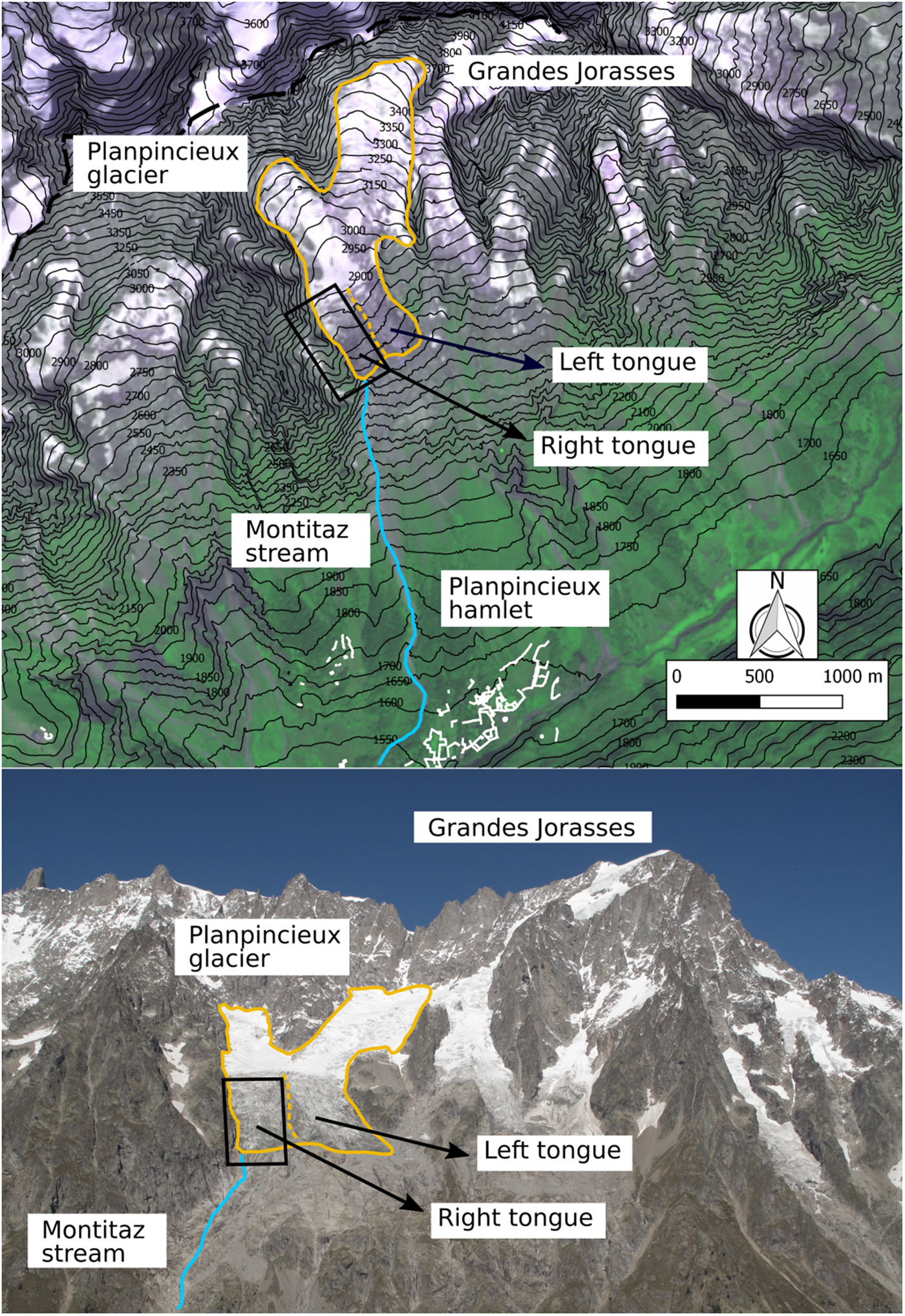
Fig. 2. Study area. The upper figure shows the right side of the Ferret valley. The limits of the Planpincieux Glacier are depicted in yellow. The dashed yellow line indicates the margin between the lower right and left lobes of the glacier. The Montitaz stream (blue line) flows from the right lobe. The buildings of the Planpincieux hamlet are marked in white outlines. The black rectangle delimits the area observed by the TELE module. The lower figure shows a panoramic picture of the Grandes Jorasses massif acquired from the monitoring station.
The left lobe is less active and not limited frontally by a bedrock step. The ice flux seems to be mainly channelled in the right lobe, which is also characterised by the presence of the Montitaz stream that flows from the glacier snout. Discharge measurements from the Montitaz stream are not available.
In the past, several major ice avalanches and outbursts of englacial water have occurred (Table 1) and, in some cases, have threatened the village of Planpincieux and damaged the road. Increased attention has been placed on this glacier since 2011 when a large crevasse opened in the lower part of the right lobe (Motta, 2016, personal communication). Since then, the glacier has been intensively monitored using different remote-sensing techniques.
Table 1. Historical records of the break-off events occurring in the Planpincieux Glacier (Report of the forest rangers of the Pré Saint Didier station of 20/02/1982, 1982; Gianbastiani, Reference Gianbastiani1983; Ceriani and others, Reference Ceriani, Fiou and Castello2010)

3. Dataset
3.1. Meteorology and glacial indexes
We collected meteorological data acquired by the Ferrachet automatic weather station (AWS) placed ~5 km far from the Planpincieux Glacier at an elevation of 2300 m a.s.l. The Ferrachet AWS represents the closest and most representative meteorological station provided by the regional meteorological service. Furthermore, we analysed the vertical profiles of the temperature and geopotential heights provided by the ERA5 reanalysis (Copernicus Climate Change Service Climate Data Store (CDS), 2017). The ERA5 is the most recent reanalysis database produced by the European Centre for Medium-Range Weather Forecasts (ECMWF) and the data are available on a regular grid at a 0.25° × 0.25° resolution and hourly frequency. Also, we considered the surface mass balance (SMB) of the glacier that is closely related to the climatic conditions. There are no available records for the mass balance of the Planpincieux Glacier.
Nevertheless, FMS periodically measures the mass balance of two glaciers in the Ferret Valley, the Toula Glacier and the Petit Grapillon Glacier (Attività glaciologiche – Fondazione Montagna sicura http://app.fondazionemontagnasicura.org/multimedia/crgv/default.asp?sezione=16&principale=32&indice=32). Both glaciers range in elevation between 2700 and 3300 m a.s.l. and have a south-easterly aspect, similar to the Planpincieux Glacier. Therefore, it is reasonable to assume that their behaviour should be comparable to Planpincieux. During the considered period, the SMB of these glaciers was positive in 2012/13 and 2013/14 and negative in the subsequent years.
3.2. Monitoring station
The lowest part of the Planpincieux Glacier has been continuously monitored for research purposes since September 2013 by a monoscopic visual-based system (VBS) that is installed on the side of the valley opposite to that of the glacier (Fig. 1) at an elevation of 2305 m a.s.l. and a distance of ~3800 m (Giordan and others, Reference Giordan2016). The VBS was developed by CNR IRPI and continuously updated since its installation. Presently, the apparatus is composed of two DSLR cameras (Canon EOS 100D and 700D) and a Raspberry Pi™ computer that manages the scheduling of the image acquisition. The cameras are equipped with different focal lengths to observe the glacier at different levels of detail. The WIDE module (focal length of 120 mm) observes the Planpincieux Glacier and its boundaries, while the ZOOM module (focal length of 297 mm) focuses on the lower right lobe of the glacier.
The cameras were installed on a concrete plinth that was placed inside a plastic shelter box. An energetic module composed of two solar panels supplies electricity to the VBS; therefore, the apparatus can work autonomously and is entirely remote-controlled. During the cold season, the system hibernates and reactivates autonomously when the snow on the solar panels clears. For more details on the developed system, please refer to Giordan and others (Reference Giordan2016).
From late October to April–June, the glacier is usually covered by fresh snow; therefore, the glacier surface is mostly invisible and the ICC processing is avoided. The images that were acquired when the glacier was covered by snow were not processed because the ice surface was not directly visible. However, in limited periods during the cold season when the glacier was uncovered by snow, we observed that the motion of the glacier was almost zero. At the operating regime, the photographs were acquired on an hourly basis, from 7:00 to 19:00.
In this study, we focused our attention on the images of the ZOOM module taken during 2014–18 from May to October and processed using ICC. In 2014, we acquired a higher frequency for the initial setup of the system. Table 2 reports the total number of collected images and the number of photographs used for the ICC. In total, we collected more than 15 000 images and almost 600 images were processed using ICC. The processed dataset corresponds to a time interval of 754 d over 5 years. To the authors' knowledge, this is the longest series of photographs acquired for a ground-based evaluation of the surface motion of an Alpine glacier.
Table 2. Total number of images acquired by the monitoring station in each year and number of images processed using image cross-correlation (ICC). The fourth column reports the number of days without images suitable processing using ICC

The acquired images were transferred using a UTMS connection to the CNR server where they are stored. The images with unsuitable illumination or unsatisfactory visibility conditions were manually discarded. The selected images were processed and the displacement maps were obtained using ICC. Moreover, possible failures were classified according to the instability process and their volume was estimated.
3.3. Ancillary data
Besides time-lapses photography, we acquired ancillary data. We collected several orthophotos provided by the WebGIS service of the Regione Autonoma Valle d'Aosta (GeoPortale – Portale dei dati territoriale della Valle d'Aosta http://geoportale.regione.vda.it/) relative to years 1999, 2005 and 2012, with ground sampling distances (GSD) of 1, 0.2 and 0.2 m, respectively. Moreover, we conducted periodic helicopter-borne surveys to directly observe the geomorphological conditions of the glacier and acquired corroborative photographic data.
On 2 April 2013, a helicopter-borne GPR (central frequency 65 MHz) survey measured the glacier thickness and allowed a description of the bedrock morphology. Furthermore, on 9 June 2014, we conducted a helicopter-borne LiDAR (sensor RIEGL LMS-Q680i) survey where we acquired a digital surface map (DSM) of the lower part of the glacier and an orthophoto with a ground sample distance (GSD) of 0.08 m. The DSM was sampled at a resolution of 0.5 m. We also conducted a terrestrial laser scanner (TLS, sensor RIEGL LMS-Z420i) survey on 2 October 2015, when we obtained a 3-D point cloud.
Moreover, we conducted four monitoring campaigns using the terrestrial radar interferometry (TRI) technique that provided the LOS-aligned measurements of the glacier motion. The results of the TRI confirmed the velocity values and the surface kinematic pattern obtained using ICC Table 3.
Table 3. Survey campaigns and datasets collected during the monitoring period

4. Methods
4.1. Meteorological analysis
The meteorological series were characterised by strong fluctuations during the 5 years of study regarding temperature and precipitation. Using the ERA5 reanalysis data, we calculated the positive degree-day (PDD) at the top height of the glacier, shown in Figure 3a, where the PDD is the cumulative sum of the daily mean positive temperatures (Hock, Reference Hock2003). We derived the temperature by assuming a constant lapse rate between two known geopotential levels. We observed that 2014 was much colder than the other years (Nimbus Web http://www.nimbus.it/clima/2014/140903Estate2014.htm) that registered similar temperatures, especially in summer. Moreover, the temperatures in September and October 2018 were much higher than usual.

Fig. 3. (a) Positive degree day at the elevation of the glacier. (b) Hourly and cumulative rainfall. (c) Snow deposition. Precipitation and snow were recorded by the Ferrachet atmospheric weather station.
The 2018 winter season was characterised by exceptional snowfalls (Fig. 3c). Therefore, the surface remained covered by snow longer than in the previous years, even though the summer was rather warm. Similarly, in 2014 and 2016, the surface cleared by mid-July, while in 2015 and 2017, the snow melted completely by the second half of June. The periods of glacier surface clearance were evaluated through visual inspection.
Concerning the liquid precipitation (Fig. 3b), 2014 was the wettest year and 2016 and 2018 were characterised by very dry warm seasons.
4.2. Glacier surface velocity measurement
ICC is a well-known methodology used for applications in the field of glaciological surveying (Scambos and others, Reference Scambos, Dutkiewicz, Wilson and Bindschadler1992; Leprince and others, Reference Leprince, Barbot, Ayoub and Avouac2007; Ahn and Box, Reference Ahn and Box2010; Fallourd and others, Reference Fallourd2010; Debella-Gilo and Kääb, Reference Debella-Gilo and Kääb2011; Vernier and others, Reference Vernier2011; Benoit and others, Reference Benoit2015; Messerli and Grinsted, Reference Messerli and Grinsted2015; Giordan and others, Reference Giordan2016; Schwalbe and Maas, Reference Schwalbe and Maas2017). It provides 2-D maps of the motion components perpendicular to the line of sight (LOS) with a sub-pixel sensitivity.
In this study, we followed the procedures described in Dematteis and others (Reference Dematteis, Giordan, Zucca, Luzi and Allasia2018) to measure the glacier surface velocity. The cross-correlation is calculated on sliding windows extracted on image pairs for estimating the displacement between the master and the slave tiles. We computed the phase correlation using the algorithm of Guizar-Sicairos and others (Reference Guizar-Sicairos, Thurman and Fienup2008), which allows for fast calculations and minimal decorrelations. The motion of the slave tile S with respect to the master tile M is extracted from the cross-correlation matrix C, obtained with

where ${\rm {\cal F}}\,{\rm and}\,{\rm {\cal F}}^{-1}$ represent the 2-D Fourier transform and inverse transform, respectively, and the symbol * represents the complex conjugate. The position of the maximum peak of C corresponds to the relative pixel shift between the two tiles.
We adopted sliding windows of 128 pixels per side with an overlap of 50% to increase data redundancy and facilitate outlier identification. Thereby, we obtained a motion field mapped on regular grids with a 3.5 m resolution. We obtained analogue results also by adopting different sliding windows sizes and overlapping ratios. We discarded the images with unsuitable illumination or visibility and we manually selected the photographs to conduct the ICC. We used one image per day, when available, acquired in conditions of diffuse illumination to minimise the noise introduced by the shadows produced by direct light (Ahn and Box, Reference Ahn and Box2010; Giordan and others, Reference Giordan2016). The shadow-related noise impeded the use of sub-daily time-lapses because it lowered the signal-to-noise ratio and increased the error (Dematteis and others, Reference Dematteis, Giordan and Allasia2019). We estimated the ICC uncertainty by analysing the displacement measured on the stable surfaces (i.e., exposed bedrock). We calculated the mean μ and Std dev. δ of the motion of 116 displacement maps, obtaining a μ = 0.1 and δ = 2.4 cm. We considered μ and δ as the estimates of the measurement accuracy and precision.
4.3. Break-off detection and volume estimation
A visual inspection of the available dataset allowed for the detection of break-offs, crevasse widening and the aperture of channels at the bedrock/glacier interface that can indicate the outburst of englacial water.
For each detected failure, we analysed the sequence of images pre- and post-event and classified the break-off according to the trigger process. The principal features that we considered in classifying the detachment processes were: (i) the collapsed volume, (ii) evidence of the water involvement in the process, (iii) the morphology of the glacier pre- and post-event and (iv) the observed shape of the detachment.
During the monitoring, we manually counted the number of collapses. In this study, we considered only those events with a volume >100 m3, even though minor and less relevant break-offs occurred almost daily. To estimate the volume of the ice detachments, we followed the subsequent procedure: we delimited the area corresponding to the collapse and we subdivided it into irregular polyhedra. Then, we manually counted the number of pixels included in the polyhedra (Fig. 4b). Similarly to Le Meur and Vincent (Reference Le Meur and Vincent2006), we made some geometrical assumptions: we assumed that the frontal and rear faces were vertical and that the bedrock underneath was regular and with a uniform slope. The bedrock inclination is assumed equal to the mean slope of the glacier surface, calculated with the DTM. Therefore, we transformed the vertex x, z picture coordinates in pixel in the spatial metric 3D coordinates x′, y′, z′, where the x ′-axis is positive rightward, the z ′-axis is positive upward and the y ′-axis is positive moving away (y is the depth dimension).

Fig. 4. Volume estimate of the break-off occurring on 9 June 2014. (a) Image of the glacier before the break-off. (b) Orthorectified nadiral photo before the failure. (c) Detail of figure (a), where the manual decomposition of the volume in irregular polyhedra is shown. The solid lines indicate the frontal edges, while the dashed lines indicate the rear (inner) edges. (d) Image of the glacier after the break-off. (e) Detail of figure (b), where the margins of the collapsed ice are depicted in yellow.
With reference to Figure 4c, we considered the lowest vertex, B 0, as the origin of the xyz ′-axes. Then, the vertex coordinates of the lower face B (the base of the polyhedron) became $x_{B_i}^{\rm ^{\prime}} = x_{B_i}-x_{B_0},z_{B_i}^{\rm ^{\prime}} = z_{B_i}-z_{B_0}$ , and $y_{B_i}^{\rm ^{\prime}} = z_{B_i}^{\rm ^{\prime}} /\tan \alpha$
 , where α is the slope angle assumed uniform and the subscript i indicates a generic point of the face B. The assumption of verticality of the frontal and rear faces implies that there is not a depth shift between the i th-point in the upper face F and the corresponding i th-point in the face B, that is, $y_{F_i}^{\rm ^{\prime}} = y_{B_i}^{\rm ^{\prime}}$
 . Finally, it holds $x_{F_i}^{\rm ^{\prime}} = x_{F_i}-x_{B_0},\; \; z_{F_i}^{\rm ^{\prime}} = z_{F_i}-z_{B_0}$
 .
.
The uncertainty E V of the volume estimation is given by the sum of three principal contributes:

where ε g is the actual validity of the geometric assumptions, ε v is the precision of the polyhedra vertexes identification and ε p is the degree of approximation in the volume subdivision in the irregular polyhedra.
ε g could be the most questionable term because it involves specific assumptions on the geometry of the break-off volumes, namely, the vertical frontal and rear faces and the regular bedrock. The DSMs from 2014 to 2015 clearly show that the glacier terminus presented a vertical ice cliff. The visual analysis of the photographic dataset revealed that the morphology of the front remained the same during the study period. A comparable morphology of the rear faces was evident after the break-off events (Figs 4a–c). Analogously, the observation of the bedrock surface did not reveal significant irregularities in the proximity of the snout.
The ε v and ε p terms are closely related and they have to do with the manual delimitation of the detached ice blocks. The delimitation is conducted by comparing the photographs before and after the failure. The expert-based teamwork and training during the 5-year study allowed us to obtain reliable results for the volume delimitation. On this basis, we conservatively estimated the uncertainty of the vertex selections as δ v = ±10 px. Therefore, considering a cube of side ℓ, we obtained an absolute error ε v = V × 3(δ v/ℓ) = 3δ vV 2/3.
Furthermore, for ε p, we evaluated the error given by the ice block division in the polyhedra with respect to the following geometric problem. We considered the ice chunk as a single convex curvilinear volume that we approximated with a polyhedron. Considering that we assume that the rear face is flat and vertical and that the base is flat and with uniform slope, the problem reduces to the case of a hemicylinder circumscribed in a parallelepiped. In such a situation, the error is ε p = ±0.21 V.
We were able to validate our volume estimation method on one occasion. Just a few hours after the LiDAR survey from 9 June 2014, a break-off occurred (Fig. 4). The collapsed block was recognisable on the orthophoto and it was easy to compute the volume from the DSM where we obtained a volume of V = 3120 + 163 m3. Adopting the image-based volume estimation, we obtained V = 3190 ± 836 m3. Therefore, the results of the proposed method are comparable and in good agreement with the reference values obtained using the DSM and georeferenced orthophoto.
4.4. Velocity-break-off relationship
We analysed the velocity time series and investigated the possible relationship between the kinematics and the break-off.
We observed several periods of rapid acceleration of the frontal glacier portion that culminated with a voluminous break-off. Therefore, we examined the behaviour during these periods using the power-law originally proposed by Flotron (Reference Flotron1977) that was adopted to predict the instant of the failures

where v(t) is the velocity at time t, v 0 is a constant velocity, t c is the time of the failure and α, m are the parameters that characterise the acceleration. We fitted Eqn (3) with the velocity from the 10 d prior to the failure; namely, t = {t c − 9, t c − 8, …, t c}. We also investigated the fit of Eqn (3) at different time intervals (i.e., from 7 to 20 d), but we did not obtain significantly different results.
Faillettaz and others (Reference Faillettaz, Pralong, Funk and Deichmann2008) observed the presence of log-periodic oscillations superimposed to the power-law behaviour of the velocity and they showed that by considering such oscillations it could be possible to improve the forecasting of the instant of failure. We did not observe any evidence on the presence of such log-periodic oscillations.
We further analysed the volume of the break-offs in relation with the glacier kinematics. We searched for a relationship between the volume of the detached ice and the velocity peaks during the active phases and between the volume and the average acceleration of the previous 5 d before the rupture. The previous 5 d corresponded to the period of sharp acceleration of the power-law curve that can be approximated to a linear trend. This could be compared to the findings of Faillettaz and others (Reference Faillettaz, Funk and Sornette2011a) that observed an energy and frequency increase in the icequake activity related to the glacier motion in the 5 d prior to the break-off.
Considering the limited number of sampled data, we conducted two stochastic analyses to assess the statistical significance of the results. The first one was a Monte Carlo simulation (Wilks, Reference Wilks2011) in which, during each iteration, we calculated the Spearman correlation coefficient r s, or rank correlation and the p-value between the velocity v and the adjusted volume $V_i^* = V_i + wE_V^i$ , where V i was the volume of the i th observation, w was a random weight in the range ± 1 and $E_V^i$
 was the estimated error of the volume V i. The Spearman correlation is more robust and resistant to a few outlying point pairs than the ordinary Pearson (or linear) correlation coefficient (Wilks, Reference Wilks2011). Therefore, it should be more significant for a dataset with a limited number of samples. The second analysis was a bootstrap analysis (Wilks, Reference Wilks2011) in which the coupled velocity-volumes used to compute the relationship were randomly selected using resubmission, that is, at each iteration, a specific couple might be excluded from the dataset, or it might be selected more times. In both simulations, we analysed the p-value using the student T-test against the null hypothesis of the zero velocity/volume relationship. We used the T-test because it has proven effective even with extremely small datasets (De Winter, Reference De Winter2013).
5. Results
5.1. Glacier evolution and instability processes
During the last decades, the Planpincieux Glacier has experienced relevant shrinkage and morphological changes. Within 2014–17, the position of the right lobe front was approximately constant (Fig. 5). Subsequently, in August 2017 a very large collapse occurred (i.e., volume >5 × 10⁴ m3) and this caused the front to move several tens of metres backwards. Furthermore, during the warm season of 2018, the front experienced a very large retreat due to ice calving. During the past years, the motion of the glacier rapidly balanced the mass loss from the margin, allowing the front to be maintained at approximately the same position. In contrast, in 2018, the reduced velocity of the glacier could not balance the ice detachments and the snout position remained at this new retreated position.

Fig. 5. The lower panels show the evolution of the position of the glacial front at the end of the warm seasons during 2014–18. The coloured lines indicate the position in each year: 2014 (cyan), 2015 (green), 2016 (yellow), 2017 (orange) and 2018 (red). The front width is ~100 m. The black dashed line indicates the large recurrent crevasse that opens each year during the warm season. The upper panels show the velocity in cm d−1 from July to September. On the left, the limits of the kinematic domains are approximately illustrated and projected on the maps with dashed black lines.
The 2018 retreat revealed a 20 m-high rock cliff orthogonal to the flow direction. Therefore, the bedrock morphology at the snout was similar to that during the past years, that is, the front ended above a steep slope gradient. Presently, this morphology makes the glacier prone to ice calving in correspondence of the second upper rock cliff. Thus, it is quite possible that the present position of the front will remain unaltered for the near future.
Besides the evolution of the terminus morphology, the kinematics of the glacier also changed during the study period. Figure 5 presents the maps of the mean daily motion of the period from 1 July to 30 September of each year. The analysis revealed that during 2014–17, the velocity values and patterns of the glacier were similar. In 2018, the glacier showed very different behaviour in two major aspects; (i) on average, the surface velocity was quite low and (ii) the patterns of the surface kinematic maps were considerably dissimilar (Fig. 5).
From the combined analysis of the evolution of the glacier morphology and kinematics, we identified different surface kinematic domains that are likely linked to the subglacial bedrock (Fig. 6d). The limit definitions were supported by the identification of different velocity regimes and by the presence of morphological features. In particular, we identified a discontinuity corresponding to a large crevasse approximately halfway on the glacier lobe, whose position and morphological shape was constant among the years (Figs 5, 6a–c). The crevasse usually opened in late August and progressively widened up to the beginning of October. In 2014, the crevasse was less evident than in the subsequent years, probably because the stresses were partially compensated by the greater glacier thickness. The volume of the ice mass under that crevasse was estimated to be on the order of 5 × 10⁵ m3.

Fig. 6. Morphodynamical scheme of the glacier. (a) Image of the glacier lobe. (b) Example map of the surface velocity. (c) Longitudinal section of the glacier (not to scale). (d) GPR profile. The limits of the kinematic domains are represented by coloured bars. The black dashed lines indicate the position of the crevasse that opens each year at the same position. The bedrock discontinuities are highlighted with black solid lines and are easily recognisable in the GPR profile. V b, V s are the basal and surface velocities, respectively.
In Figures 5, 6a–c, we show the limits of the kinematics domains. Sector A is the frontal area that is characterised by the fastest surface velocity and the highest break-off activity. Sector B corresponds to the portion between sector A and the crevasse placed approximately halfway on the lobe. Sector C is the steep area above the aforementioned crevasse and sector D is the gentle upper area.
The daily acquisition of a high-resolution image dataset was fundamental for the detailed description of the phenomena that affected the study area. During the warm season, the glacier snout was subjected to intensive ice calving that manifested three processes that led to break-offs: (i) disaggregation, (ii) slab fracture and (iii) water tunnelling.
Disaggregation (Pralong and Funk, Reference Pralong and Funk2006) of the frontal ice cliff (Fig. 7a) occurred most frequently and was usually characterised by a series of limited volume collapses usually on the order of 102 − 103 m3 that occurred in limited portions of the terminus. This process was activated by the progressive toppling caused by the movement of the glacier beyond the frontal step. The continuous disaggregation limits the presence of large unstable masses near the glacier margin.

Fig. 7. Instability processes. Panel (a) On the left, the disaggregation detachment scheme is shown. On the right, images of the pre- and post-event are shown. Panel (b) On the left, the slab break-off scheme is shown. On the right, images of the pre- and post-event are shown. Panel (c) On the left, the water tunnelling scheme of the break-off is shown. The light-blue line indicates englacial water. On the right, the pre- and post-event images are shown. The yellow lines delimit the collapsed volume before (left photo) and after (right photo) the break-off events. The front width is ~100 m.
Slab fractures are the second type of detachment and are triggered by the propagation of a fracture that reaches the bedrock (Pralong and Funk, Reference Pralong and Funk2006), which fosters increased ice sliding, causing the detachment of an ice lamella. The failures usually involve large portions of the glacier lobe, with volumes on the order of 104 m3 and their activation is quite rapid. In many cases, we noticed a velocity increment before the detachment, related to the progressive spreading of the fracture. After such events, the subglacial bedrock remains almost uncovered (Fig. 7b).
Water tunnelling is the third instability process that has been observed during a few events when the ice collapsed with the presence of substantial volumes of water. The collapses revealed cavities beneath the glacier body (Fig. 7c). Such cavities can indicate the presence of a channelled hydraulic network where the water flows in river-like tunnels, that is, Röthlisberger-channels (Röthlisberger, Reference Röthlisberger1972). In this situation, the pressure exerted by the water directly on the frontal ice face can provoke detachments of considerable volume; furthermore, the cavities produced by the erosion and melting of the englacial water can collapse. We observed channels with a diameter of more than 10 m, possibly indicating a very large amount of water inside and beneath the glacier body. During the event on 1 August 2017, in concomitance with a rainstorm, an impressive water spurt that came out from the snout base was directly observed (Motta, 2016, personal communication). In the past, similar phenomena occurred when great glacier outbursts were accompanied by floods that endangered the Planpincieux village (Table 1).
Moreover, as depicted in Figure 8, we analysed the average magnitude of the events triggered by the different instability processes. As expected, the slab fracture type involves the greatest volume of ice, on the order of 104 m3. The water tunnelling failures were less frequent and the volume was rather variable. The disaggregation process usually involved less ice, although a few events had volumes over 5 × 10³ m3.

Fig. 8. (a) Boxplot of the break-off volume caused by different processes. The number of disaggregation, slab fractures and water tunnelling events is 151, 13 and 9, respectively. (b) Total amount of collapsed volume. (c) Number of break-off events.
Considering the ensemble of all the break-off events, it appears that, even though the collapses smaller than 1000 m3 are more than half of the total number, they account for only 10% of the total volume approximately. On the contrary, the few collapses larger than 10 000 m3 contribute for more than 50% of the total volume collapsed (Fig. 8).
5.2. Glacier kinematics
According to the identification of the different sectors, we analysed the evolution of the mean velocity of sectors A and B. In Figure 9, we present the time series of the two sectors during the considered periods and the occurrence of the break-off phenomena, distinguishing their different geneses. We highlighted the periods that are characterised by a strong acceleration of sector A.

Fig. 9. Time series of the daily velocity of sectors A and B during 2014–18. The collapse events are displayed as coloured dots according to the instability process: disaggregation events are black, slab fractures are red and water tunnelling failures are cyan. The dimension of the black circles is proportional to the volume of the break-off. The grey rectangles indicate the active phases that culminate with slab-induced failures. The red rectangles indicate potential active phases whose evolution was probably interrupted by temperature decreases and snowfalls; these accelerations culminated with disaggregation events.
The comparison of the time series among the years showed that, on average, the maximum registered velocity of sector A progressively increased from 2014 to 2017 and lowered in 2018. Table 4 presents the maximum velocities of sector A for each year.
Table 4. Maximum velocity, cumulative volume of collapsed ice and number of events of the different processes in each year

Concerning glacier break-off, 2014 and 2018 registered more events, while the global volume amount of the ice failures was at a maximum in 2014 and 2017. Table 4 shows the total number of observed collapses with estimated volume >100 m3 in each year and the cumulative volume.
Furthermore, Figure 9 shows the presence of a particular behaviour in the glacier lobe evolution. It is possible to identify a series of velocity fluctuations that always occurred during the second half of the warm season. These periods of abrupt acceleration were particularly evident in 2015, 2016 and 2017. In late 2018, two such fluctuations were noticed, although the acceleration was less pronounced, while in 2014, the seasonal behaviour of the velocity increased from mid-June to mid-August, where it reached the maximum value and then slowly decreased without the occurrence of the active phases.
Interestingly, each speed-up period culminated in a voluminous break-off, usually a slab type. The process of slab fracture adapts well to such velocity behaviour as it involves a progressive crevasse opening, causing an increase in the sliding motion. In a few cases (highlighted in red in Fig. 9), the acceleration process was interrupted by significant temperature decreases and the active phase ended with a disaggregation failure.
For each active phase, we fitted Eqn (3) with the velocity data from the 10 d prior to the ruptures (highlighted in Fig. 9) with the volume of the corresponding break-off. We present the results of the fit in Figure 10 and the regression statistics in Table 5. We observed that the behaviour of the active phases was in good agreement with the power-law regression (Flotron, Reference Flotron1977).

Fig. 10. Active phases of the 10 d before slab fractures collapses (a, c, e, f, g, i). Active phases of the 10 d before disaggregation collapses (b, d, h). The circles represent the observed velocity, the solid lines are the power-law fit and the dotted lines are the linear fit of the previous 5 d of the active phases.
Table 5. The table reports the dates of the break-offs during the active phases. The dates with asterisks refer to disaggregation type failures. The coefficient of determination (R2) and RMSE were computed for the power-law fit of Eqn (3) using the 10 d before the break-off. The p-value was computed against the null-hypothesis of the linear fit

Besides the analysis of the power-law behaviour of the active phases, we also investigated the relationship between their maximum velocity and the volume of the break-off events (Fig. 11c). As expected, the fastest active phases were associated with slab fracture-induced failures that are the most voluminous detachments.

Fig. 11. (a) Spearman correlation coefficient between the velocity and volume obtained with bootstrap (bst) and Monte Carlo (MC) analyses. (b) p-value of the spearman correlation for the Monte Carlo analysis. (c) Relationship between the velocity and break-off volume.
The statistical significance of the monotonic relationship is supported by the analysis of the 1000-iteration bootstrap and Monte Carlo analyses. In fact, in both cases, the Spearman correlation coefficient assumed values above 0.7 on average (Fig. 11a). Moreover, the p-value computed within the Monte Carlo simulation revealed that the relationship was verified at a 0.02 significance. This result is not trivial because it can permit a quantitative estimation of the possible volume of break-off events. Conversely, we did not discover any significant relationship between the acceleration and the volume.
Furthermore, we noticed that each active phase that ended with failure was characterised by an average acceleration over 5 d α ≥ 3 cm d−2 and by an initial velocity v 0 ≥ 30 cm d−1 (Table 6). Considering these acceleration and velocity values, only in one case (18 August 2017) we observed higher velocity and acceleration without the occurrence of a collapse. In that circumstance, we identified the detachment of an ice chunk from the glacial body that remained leaned onto the bedrock, separated from the main glacial mass. Since we did not register a paroxysmal collapse, we did not categorise it as a break-off. Nevertheless, even in this case, the velocity fluctuation was caused by an ice detachment from the main body.
Table 6. Dates of potential active phases and volume of the relative break-off. α is the angular coefficient (i.e., the acceleration) of the linear fit of 5 consecutive days and v0 is the velocity at the first day of each potential active phase. The rows in italic refer to a disaggregation detachment. The date with asterisks indicates events that did not culminate in a break-off

6. Discussion
The observations during the 5-year monitoring study allowed for the acquisition of specific knowledge regarding the Planpincieux Glacier and its dynamics. In this section, we report the principal features of the glacier that were identified during the analysis of the surface kinematics, the instability dynamics and the morphology evolution.
6.1. Instability processes
In the Planpincieux Glacier, we identified three main instability processes: disaggregation, slab fracture and water tunnelling. The former two are related to the glacier geometry; disaggregation is typical of ice cliffs (Diolaiuti and others, Reference Diolaiuti, Smiraglia, Vassena and Motta2004; Pralong and Funk, Reference Pralong and Funk2006; Deline and others, Reference Deline, Gardent, Magnin and Ravanel2012). In the Mont Blanc massif, disaggregation is frequent in warm glaciers and it involves small volumes (usually <1000 m3) (Alean, Reference Alean1985b; Deline and others, Reference Deline, Gardent, Magnin and Ravanel2012). Disaggregation acts as a stability process because it does not allow the formation of a homogeneous ice chunk that could collapse at once. Larger events are triggered by slab fracture process. Slab fractures occur in glacier termini that end in correspondence of a bedrock cliff (Alean, Reference Alean1985a; Pralong and Funk, Reference Pralong and Funk2006) and they can induce a larger volume that can reach a few hundred thousands cubic metres (Alean, Reference Alean1985a; Huggel and others, Reference Huggel, Haeberli, Kääb, Bieri and Richardson2004). On the contrary, water tunnelling is related to the presence of englacial liquid water, which can form R-channels (Röthlisberger, Reference Röthlisberger1972). Such tunnels might develop pockets that can provoke water outburst and subsequently they can collapse. Water tunnelling rarely yields surface velocity raise, therefore it is more difficult to recognise break-off precursors with the analysis of the glacier kinematics. According to Faillettaz and others (Reference Faillettaz, Funk and Vincent2015), a possible solution for the acquisition of representative data to identify this process is the analysis of the seismicity and water discharge.
We conducted a meteorology analysis to evaluate the effects of temperature and precipitation on the activation of velocity fluctuations and break-offs. The atmospheric conditions should have a strong influence on glacier stability because they force ice melting and hence water percolation. Nevertheless, we did not find a clear relationship with the active phase occurrence. Probably, this could be ascribed to the nondiffuse configuration of the hydraulic system, which is one of the primary forcings for glacier sliding (Bjornsson, Reference Bjornsson1998).
In Figure 6, we presented a conceptual longitudinal section of the glacier. According to the identification of different kinematic and morphological domains, we divided the right glacier lobe into four sectors with different velocities. These velocity differences and the limits of the zones are likely influenced by the topography of the bedrock, as the limits of such domains are positioned along corresponding bedrock discontinuities detected by the GPR. In fact, it is known that the geometry of the bedrock is one conditioning factor for the creation of crevasses (Pralong and Funk, Reference Pralong and Funk2006). The presence of different kinematic domains with dissimilar velocities indicates the action of strong tensile stresses that cause the aperture of crevasses. The induced strain rates can be identified in the velocity gradient between different sectors. In Figure 9, we can observe that the strain rate increases during the active phases, while it remains close to zero during the normal regime. According to our findings, we identified a critical scenario that could provoke a very large rupture in the hypothetical case where the sectors A and B accelerate together and move at the same rate. Such a condition implies that the stresses are concentrated in correspondence of the crevasse above sector B. The occurrence of slab fractures in this part of the glacier would involve an estimated volume of more than 5 × 10⁵ × m3.
6.2. Interannual variability of glacier kinematics
Thanks to a dataset characterised by a high temporal and spatial resolution, we detected a relevant variability in the glacier kinematics. Specifically, we identified two different regimes in the velocity evolution. The first was in 2014, where an evident seasonal trend with a progressive velocity increment from May to August was identified. It reached a maximum value in August and then slowly decreased together with the diminished temperature. The break-offs were homogeneously distributed during the warm season and the volume of the detachments was not linked to the velocity. A different behaviour was observed in 2015–17, when the kinematics presented a series of velocity fluctuations and an empirical relationship between the velocity and the volume of the break-off. Moreover, we also registered a remarkable positive trend in the glacier activity year-by-year. In 2018, the glacier showed a quite limited activity for most of the warm season. The motion and instabilities increased in September and the glacier remained rather active up to the end of October, showing nonregular behaviour compared to the previous years. The reason for the reduced motion in 2018 is probably due to the considerable snow cover that cleared in late July and resulted in a delayed beginning of the summer sliding process. The study of the evolution of the glacier started in 2014, which was characterised by different kinematics. Since we did not have data before 2014, we are not able to know the glacier behaviour prior the 2014 and if the 2014 behaviour was anomalous. Probably, the dissimilar behaviour between 2014 and the subsequent years can be ascribed to a colder melting season and a positive mass balance. Low temperatures and a large amount of snow that partially covered crevasses even during the summer season limited the water percolation. Conversely, since 2015 the glacier surface was much crevassed and the melted water could flow easily through the fractures and reach the bedrock, increasing the glacier sliding.
6.3. Seasonal behaviour: velocity fluctuations and break-offs
In 2015, 2016, 2017 and 2018, the surface velocity showed a peculiar behaviour that was characterised by a sequence of fluctuations lasting for 2–3 weeks on average. These fluctuations always occurred during the second half of the warm seasons when the motion of the glacier reached its maximum activity. In correspondence of the oscillation peaks, we always registered a break-off event of relevant volume. Recalling the study of Röthlisberger (Reference Röthlisberger and Kasser1981), Faillettaz and others (Reference Faillettaz, Funk and Vincent2015) described similar active phases in the Allalingletscher Glacier. They noticed that on several occasions the active phases did not culminate with an ice break-off, but that the collapses only occurred during the accelerations. Therefore, they stated that such active phases are necessary but not sufficient condition for the occurrence of ice ruptures. Conversely, we observed that large break-offs always occur, but not exclusively, during such speed-up periods. Therefore, the active phases can be considered a sufficient but not necessary condition for the occurrence of ice ruptures. Faillettaz and others (Reference Faillettaz, Funk and Vincent2015) and Vincent and Moreau (Reference Vincent and Moreau2016) observed active phases occurring at the end of the warm season due to the action of the subglacial water flow when the partial closure of the hydraulic system can cause an increase in interstitial pressure. Hence, diminished water discharge from the terminus might be a precursor of a possible break-off event. In the case of the Planpincieux, although we cannot provide a quantitative analysis of the water discharge, we did not detect any evident change in the water discharge from the snout through visual analysis of the images.
In the presented case study, the registered surface velocity raise that precedes a break-off is due to the positive combination of rotational movement of the ice chunk with the translative sliding of the glacier. Such behaviour was already described by Iken (Reference Iken1977), which measured with a kryokinemeter and numerically modelled the displacements of a 20 m-thick ice lamella. She showed that the fracture opened in the zone of maximum tensile stress and then propagated through the entire ice thickness. Then, the ice chunk collapsed when the centre of gravity moved past the supporting edge of bedrock. Notably, its model showed that the velocity reached by the ice chunk is proportional to the volume, as confirmed by our observations (Fig. 11). The deceleration that follows the break-off derives from the lower stresses due to mass loss, which yielded strain rate decrease. The ice acceleration before an ice break-off has been already described in other studies (Iken, Reference Iken1977; Le Meur and Vincent, Reference Le Meur and Vincent2006; Vincent and others, Reference Vincent, Thibert, Harter, Soruco and Gilbert2015; Faillettaz and others, Reference Faillettaz, Funk and Vagliasindi2016). In the majority of the studies, the observations concerned cold-based hanging glaciers, for which the dynamics of the failure follows a power-law behaviour and the time of the failure can be forecasted (Faillettaz and others, Reference Faillettaz, Funk and Vagliasindi2016). The lower portion of the Planpincieux Glacier is wet-based and the mechanisms that drive the sliding are more complex and difficult to investigate. Therefore, at the state of the art, the break-off prediction is not achievable in this case. Nevertheless, we have found kinematic thresholds that characterise the activation of a velocity fluctuation that always leads to a break-off. Velocity thresholds for early warning purposes have also been defined by Margreth and others (Reference Margreth2017) based on heuristic criteria. In the Taconnaz Glacier, Vincent and others (Reference Vincent, Thibert, Harter, Soruco and Gilbert2015) also identified thresholds of critical volume that could lead to major collapses. The kinematic thresholds we determined for Planpincieux Glacier can help in the identification of break-off precursors and the monotonic velocity/volume relationship can be adopted to provide a quantitative estimation of possible collapses. The results of this study may have a profound relevance toward the assessment of alert strategies and civil protection as we present a criterion (i.e., thresholds of velocity and acceleration) that defines the occurrence of potential active phases that culminated with a break-off in 90% of the cases. Even if we assume that these results should be considered site-dependent, the scientific approach we followed can be reproduced and the methodology can be applied in different glaciers or contexts.
In October 2018 and in September 2019, we observed that sectors A and B were moving together and this was considered a critical condition that could evolve in a large ice break-off. The analysis of the kinematics in 2018 revealed low strain rates and velocity; therefore, the risk of a large break-off was limited. Conversely, in 2019, the strain rates were very high and they provoked the aperture of a large crevasse that underlined an ice lamella of more than 2.5 × 10⁵ m3 (https://www.nytimes.com/2019/09/25/world/europe/glacier-italy-climate-change.html).
7. Conclusions
This paper presents the application and potential of an image-based remote-sensing approach for glacier monitoring. In particular, we were able to observe and classify the main instability processes at the Planpincieux Glacier terminus. Moreover, we estimated surface kinematics and ice break-off volumes and we found a monotonic relationship between the velocity peaks and the volume of the collapses. The glacier annual maximum velocities ranged between 50 and 113 cm d−1. We observed a few break-off events per year with volumes larger than 10 000 m3 and in one circumstance the estimated volume was ~55 000 m3.
We presented the results of the image-based monitoring of the Planpincieux Glacier during the melt seasons of 2014–18. The proposed low-cost monitoring system was used to study the evolution of the Planpincieux Glacier and it is part of the wider open field laboratory that monitors the evolution of the glaciers on the Italian side of the Grandes Jorasses massif using various monitoring techniques (Faillettaz and others, Reference Faillettaz, Funk and Vagliasindi2016; Dematteis and others, Reference Dematteis, Giordan, Zucca, Luzi and Allasia2018). The original aim of the monitoring plan was the study of the glacier evolution and the possibility to identify precursors of large ice avalanches. The availability of a long sequence of daily images allowed us to detect the most relevant processes that occurred at the glacier terminus. In particular, the study focused on the break-off processes of the right glacier lobe. We conducted a visual analysis and classified three different categories of instability processes related to the geometry (disaggregation and slab fracture) and to the hydraulic system (water tunnelling). Moreover, we measured the surface velocity using an ICC procedure. Visual inspection and ICC coupling allowed at identifying the kinematic sectors in the ice tongue and their relative velocities. This is essential for a more detailed analysis of the glacier evolution and the study of break-off events. In particular, we determined kinematic thresholds, that is, velocity >30 cm d−1 and acceleration >3 cm d−2, for the activation of speed-up periods that provoke collapse with high probability (i.e., 90% of the cases). Moreover, we found a direct monotonic relationship between the velocity of the frontal part of the glacier lobe and the volume of ice failures that allows the quantification of the collapsed ice amount. This link is evident especially for slab fractures, which have the largest detachment volume of the three break-off process categories. The identification of this relationship can help in the quantitative assessment of the unstable areas and for warning purposes.
Licenses
The manuscript contains modified Copernicus Atmosphere Monitoring Service information from 2018. Neither the European Commission nor the ECMWF is responsible for any use that may be made of the Copernicus information or the data it contains.
Acknowledgements
We are grateful for the relevant and constructive suggestions of two anonymous reviewers and the Scientific Editor Dr Rachel Carr for its support during the manuscript preparation that helped to improve our work and increased the overall paper quality.
Author contributions
D. Giordan conceived the study. N. Dematteis processed the data. D. Giordan and N. Dematteis dealt with the analysis and wrote the paper. D. Giordan and P. Allasia developed the monitoring apparatus and collected the data. E. Motta contributed with valuable advices toward the paper preparation.
Conflict of interests
The authors declare that they have no conflict of interest.


 Open access