


Introduction
The global population of glaciers has been identified as a key contributor to recent (Gardner and others, Reference Gardner2013; Vaughan and others, Reference Vaughan2013; Zemp and others, Reference Zemp2019) and near-future projected sea-level rise (Meier and others, Reference Meier2007; Radić and others, Reference Radić2014; Hock and others, Reference Hock2019), with minimum projected contributions of 94 ± 25 mm of sea-level rise from 2010 to 2100 under the IPCC-AR5 RCP 2.6 scenario (Hock and others, Reference Hock2019). Outside of the glaciers peripheral to the Greenland and Antarctic ice sheets, mass loss from glaciers in Arctic Canada and the Alaska–Yukon region dominates recent and projected sea-level rise (Radić and others, Reference Radić2014; Wouters and others, Reference Wouters, Gardner and Moholdt2019; Zemp and others, Reference Zemp2019). The 25 267 km2 ice cover of the St. Elias Mountains (Kienholz and others, Reference Kienholz2015) accounts for ~38% of ice-covered area in the Alaska–Yukon region (Pfeffer and others, Reference Pfeffer2014), and comprises the largest non-polar icefield in the world. Estimates of mass-balance rates in this area range from −0.47 ± 0.09 m w.e. a−1 (1962–2006) for the St. Elias and Wrangell Mountains together (Berthier and others, Reference Berthier, Schiefer, Clarke, Menounos and Rémy2010), to −0.63 ± 0.09 m w.e. a−1 (2003–07) for the St. Elias Mountains alone (Arendt and others, Reference Arendt2008), to −0.78 ± 0.34 m w.e. a−1 (1958–2008) for glaciers confined to Yukon (Barrand and Sharp, Reference Barrand and Sharp2010). In addition to their longstanding cultural and historical significance (Cruikshank, Reference Cruikshank2001), glaciers of Yukon's St. Elias Mountains have motivated scientific research dating back to 1935 (Clarke, Reference Clarke2014).
This study focuses on the Kaskawulsh Glacier, a large land-terminating glacier on the continental side of the St. Elias Mountains. Recent retreat of the Kaskawulsh Glacier has had a cascade of unanticipated consequences, beginning with the 2016 rerouting of runoff destined for the Bering Sea to the Gulf of Alaska (Shugar and others, Reference Shugar2017). This hydrological reorganisation has directly impacted local communities through metres of lowering of downstream Lhú’áán Män (Kluane Lake) (e.g. McKnight, Reference McKnight2017) and degradation of local air quality arising from dust mobilised from the abandoned Ä’äy Chú (Slims River) valley (Bachelder and others, Reference Bachelder2020). In addition to its profound effects on local hydrology, the Kaskawulsh Glacier is also an excellent indicator of regional glacier change: it represents ~9% of glacier-ice volume in Yukon (Farinotti and others, Reference Farinotti2019), and experienced rates of mass loss from 1977 to 2007 nearly identical to those calculated for the St. Elias Mountains as a whole (Berthier and others, Reference Berthier, Schiefer, Clarke, Menounos and Rémy2010). It is also an ideal target for geodetic mass-balance measurements, being one of few large glaciers in the region not known to surge (Post, Reference Post1969) and therefore free of the complications associated with rapid, large-scale mass redistribution (e.g. Arendt and others, Reference Arendt2008).
New geodetic and geophysical data present a unique opportunity to investigate a decade of change over the Kaskawulsh Glacier. The first objective of this study is therefore to compute the geodetic mass balance using recently acquired SPOT5/6/7 data to assess glacier mass balance. The second objective is to assess the state of dynamic adjustment to the mass (im)balance and to estimate committed mass loss from the Kaskawulsh Glacier. We do this by comparing measured ice fluxes – estimated using data from the first spatially extensive ice-penetrating radar (IPR) survey of the glacier and NASA MEaSUREs ITS_LIVE surface velocities (Gardner and others, Reference Gardner, Fahnestock and Scambos2019) – to balance fluxes determined using a fully distributed mass-balance model. Hence, we explore discrepancies between internal mass redistribution and climate-driven surface mass-balance change to evaluate the current extent of this dynamic adjustment. The final objective of this study is to use the continuity equation to evaluate discrepancies between modelled, observed and derived quantities used to compute the mass budget. The results of this study help us characterise the Kaskawulsh Glacier's response to a negative balance regime, and to place a minimum bound on the committed glacier mass loss under current climate.
Study area
The St. Elias Mountains (Fig. 1) are characterised by steep terrain, extending from sea level in the Gulf of Alaska to some of the highest peaks in North America over <100 km. This topographic setting results in steep environmental gradients (e.g. Clarke and Holdsworth, Reference Clarke and Holdsworth2002) due to orographic interruption of atmospheric moisture transport and elevation-dependent temperature lapse rates (e.g. Marcus and Ragle, Reference Marcus and Ragle1970; Williamson and others, Reference Williamson2020a). These variable environmental conditions are associated with a full spectrum of glacier thermal and dynamic regimes, including a significant population of surge-type glaciers (e.g Post, Reference Post1969; Clarke and others, Reference Clarke, Schmok, Ommanney and Collins1986). The Kaskawulsh Glacier is ~70 km long, has an area of 1096 km2 and comprises three major branches (referred to as the North, Central and South Arms). One large tributary (Stairway Glacier) merges between the confluences of the South and Central Arms, while one smaller unnamed tributary joins the Central Arm above Stairway Glacier and has been known to surge (Foy and others, Reference Foy, Copland, Zdanowicz, Demuth and Hopkinson2011). The glacier flows generally eastwards from its divides in the Icefield Ranges (at elevations of 2578, 2091 and 2393 m a.s.l., respectively, for the North, Central and South Arms). The glacier terminus sits at an elevation of ~759 m a.s.l. at the head of two major river valleys: the Ä’äy Chú (Slims River), which flows north to Lhú’áán Män (Kluane Lake), and the Kaskawulsh River, which flows southeast to its confluence with the Alsek River. The 3027 km2 Kaskawulsh Glacier catchment also includes numerous smaller glaciers at elevations ranging from ~800 to ~3500 m a.s.l. The Kaskawulsh Glacier is currently retreating, with its Holocene maximum located ~25 km to the north and occurring in the early- to mid-17th century (Johnson, Reference Johnson1972; Reyes and others, Reference Reyes, Luckman, Smith, Clague and Van Dorp2006). Foy and others (Reference Foy, Copland, Zdanowicz, Demuth and Hopkinson2011) estimate 1–2 km of retreat since 1955 using satellite imagery and historical air photos. The most recent estimate of glacier-wide mass balance is −0.35 m w.e. a−1 (−0.37 Gt a−1) for 1995–2013 made using airborne laser altimetry (Larsen and others, Reference Larsen2015). Though it has never been thoroughly studied, the thermal regime of Kaskawulsh Glacier has been described as temperate (e.g. Foy and others, Reference Foy, Copland, Zdanowicz, Demuth and Hopkinson2011; Darling, Reference Darling2012; Herdes, Reference Herdes2014) likely based on measurements of ice temperature at depths of 15–24 m (Holdsworth, Reference Holdsworth1965; Anderton, Reference Anderton1967, Reference Anderton1973), though there is evidence of both temperate and polythermal ice in the accumulation area (Holdsworth, Reference Holdsworth1965).

Fig. 1. Study area (red box, inset) and overview of Kaskawulsh Glacier. Kaskawulsh Glacier highlighted in blue (regions where surface is darker are debris-covered), with major tributaries labelled: North Arm (NA), Central Arm (CA), Stairway Glacier (SW), South Arm (SA). Also shown are locations of automatic weather stations (magenta triangles) and Eclipse Icefield site with multi-annual accumulation data (blue triangle) (Kelsey and others, Reference Kelsey, Wake, Yalcin and Kreutz2012). Red-dashed lines indicate position of balance terminus position, referred to in the ‘Analysis and interpretation’ section. Black contours are m a.s.l. and coordinates are UTM Zone 7 North. Background image: Copernicus Sentinel data 2017. Retrieved from Copernicus Open Access Hub 01/11/17.
Geodetic mass balance, 2007–18
Elevation changes and mass balance from 2007 to 2018 are derived from optical satellite stereo-imagery acquired by the SPOT5-HRS, SPOT6 and SPOT7 sensors. The 2007 topography is derived by mosaicking two SPOT5 DEMs acquired during the SPIRIT project (Korona and others, Reference Korona, Berthier, Bernard, Rémy and Thouvenot2009) on 3 and 13 September 2007. The 2018 topography is derived from SPOT6 and SPOT7 DEMs acquired on 17 and 31 August, 18 September and 1 October 2018. We generate SPOT6/7 DEMs using the Ames Stereo Pipeline (Lacroix, Reference Lacroix2016; Shean and others, Reference Shean2016; Berthier and Brun, Reference Berthier and Brun2019).
The processing of the DEMs follows the workflow presented in Berthier and Brun (Reference Berthier and Brun2019). A horizontal pixel size of 20 m is chosen here for the analysis. All DEMs are coregistered to TanDEM-X (Rizzoli and others, Reference Rizzoli2017) on stable terrain following Berthier and others (Reference Berthier2007), masking out glacierised areas using the Randolph Glacier Inventory (RGI) v6.0 (Pfeffer and others, Reference Pfeffer2014; Kienholz and others, Reference Kienholz2015). In 2007, the 3 September DEM is preferred because it covers most of Kaskawulsh Glacier; its gaps are filled using the 13 September DEM. In 2018, the 1 October DEM is the primary source of elevation data with successive gaps filled by the 17 August, 31 August and 19 September DEMs.
To extract elevation change with altitude and compute the mass balances of individual glaciers, we exclude data outside ±3 standard deviations from the mean elevation difference in each 50 m altitude interval for each glacier (Berthier and others, Reference Berthier, Arnaud, Baratoux, Vincent and Rémy2004). We also exclude pixels where the surface slope, calculated from the TanDEM-X DEM, is larger than 45°. The total volume change is calculated as the integral of the mean elevation difference in each 50 m band over the total area–altitude distribution. The mass balances are then derived using a volume-to-mass conversion factor of 850 kg m−3 (Huss, Reference Huss2013) and dividing by the time interval (11 years in this case).
Errors in elevation difference are estimated based on the residuals in the overlapping area of the coregistered 2007 and 2018 DEMs, a method referred to as triangulation (Nuth and Kääb, Reference Nuth and Kääb2011; Paul and others, Reference Paul2015). We find mean absolute residuals of ~1.2 m, which, given the 11-year time interval, translate into 0.11 m a−1. Given the size of Kaskawulsh Glacier, we assume that random errors are negligible. The spatial coverage with valid elevation-change measurements reached ~70%. To account for uncertainties due to gap filling, we conservatively multiply these errors by a factor of five for the remaining 30% of the area (Berthier and others, Reference Berthier2014). An uncertainty of ± 60 kg m−3 is assumed for the volume-to-mass conversion factor (Huss, Reference Huss2013).
Figure 2 illustrates nearly pervasive thinning of the Kaskawulsh Glacier from 2007 to 2018 that generally decreases with elevation. The maximum thinning rates exceed 7.5 m w.e. a−1 roughly 5–10 km upglacier of the terminus. The influence of medial moraines is evident in the map of elevation change, but there does not appear to be a simple relationship between debris cover and glacier thinning. Although it may be tempting to ascribe some of the reduced thinning near in the lowermost 5 km of the glacier to debris cover, this relationship is not easily corroborated elsewhere. The most notable exception to the observation of pervasive thinning is an area of pronounced thickening in the upper reaches of the tributary to the Central Arm that is known to surge (Foy and others, Reference Foy, Copland, Zdanowicz, Demuth and Hopkinson2011), and is likely building up mass during its quiescent phase. Heterogeneous patches of thinning and thickening occur at elevations above 1900 m a.s.l. in the four tributaries. The data in Figure 2 yield a 2007–18 average glacier-wide geodetic mass balance of −0.46 ± 0.17 m w.e.

Fig. 2. Elevation change of Kaskawulsh Glacier, 2007–18, derived from SPOT5-HRS, SPOT6/7 optical stereo imagery. Hatched areas indicate interpolated values for gaps >1 km2. The bold black line corresponds to zero elevation change. Coordinates are UTM Zone 7 North. The inset shows colour scale overlain by elevation change vs elevation (dark grey line = mean, light grey shading = standard deviation) calculated with 100 m elevation bins (left) and histogram of elevation change (right). Background image: Copernicus Sentinel data 2017. Retrieved from Copernicus Open Access Hub 01/11/17.
Modelled surface mass balance
We model the 3-hourly distributed surface mass balance $\dot {b}_{\rm sfc}\lpar x\comma\; \, y\rpar$ of the Kaskawulsh Glacier as

where $\dot {c}_{\rm sfc}\lpar x\comma\; \, y\rpar$ is the distributed surface accumulation rate and $\dot {a}_{\rm sfc}\lpar x\comma\; \, y\rpar$
 is the distributed surface ablation rate. Modelling the surface mass-balance requires four steps (Fig. 2): (1) assembling the geometric, meteorological and mass-balance data used as model inputs, (2) calculating radiation, and downscaling/bias-correcting precipitation and temperature, (3) tuning the melt model using observational targets and (4) calculating the surface mass balance and its uncertainty for the study time period (Fig. 3).

Fig. 3. Mass-balance model workflow, including (from top to bottom) assembly of model inputs, pre-processing of meteorological variables, model tuning and using the tuned model to calculate mass balance.
Mass-balance model
We assume that surface ablation is equivalent to melt, which is determined using an enhanced temperature-index model originally developed by Hock (Reference Hock1999) that incorporates calculated potential direct clear-sky radiation. We drive the melt model with downscaled and bias-corrected regional reanalysis air-temperature data. Accumulation is determined by downscaling and bias correcting regional reanalysis surface precipitation data, which are then partitioned into rain and snow using a prescribed rain-to-snow threshold temperature.
Ablation
Melt (M) is calculated as (Hock, Reference Hock1999)
where T is the 3-hourly temperature obtained from downscaled temperature and geopotential data (described below) across the Kaskawulsh Glacier catchment, I is the potential direct clear-sky radiation, MF is the melt factor and a snow/ice are the radiation factors for snow and ice, respectively. MF and a snow/ice must be empirically determined.
Accumulation
A statistical downscaling approach adapted from Guan and others (Reference Guan, Wilson and Xie2009) is applied to the regional reanalysis surface precipitation input, with a prescribed rain-to-snow temperature threshold (e.g. Sælthun, Reference Sælthun1996; Kienzle, Reference Kienzle2008; Clarke and others, Reference Clarke, Jarosch, Anslow, Radić and Menounos2015) of 1°C (Jóhannesson and others, Reference Jóhannesson, Sigurdsson, Laumann and Kennett1995). This threshold value is selected to reduce the difference between modelled and measured accumulation at multiple snow depth and density measurement locations throughout the study time period (considering threshold values of 0–2°C). Refreezing of meltwater within the seasonal snow pack is accounted for by implementing a distributed thermodynamic parameterisation adapted from Janssens and Huybrechts (Reference Janssens and Huybrechts2000): for every hydrologic year in the study time period, total energy consumed by refreezing is approximated as a proportion (P r) of the seasonal snow pack:
with c the specific heat capacity of ice, L the latent heat of fusion, T mean the local mean annual air temperature (°C), C mean the local mean annual accumulation for the study time period and d the thickness of the thermal active layer raised to the melting point by refreezing. This is a simple thermodynamic parameterisation of the cold content of the upper snowpack that has been used to estimate the thickness of superimposed ice in ice-sheet models (Huybrechts and de Wolde, Reference Huybrechts and de Wolde1999). We set the value of d to 2 m (Oerlemans, Reference Oerlemans1991; Janssens and Huybrechts, Reference Janssens and Huybrechts2000), which has been used for the parameterisation of refreezing in modelling studies of glaciers in Western Canada (Clarke and others, Reference Clarke, Jarosch, Anslow, Radić and Menounos2015).
Model inputs
Digital elevation model and glacier geometry
We use the TanDEM-X radar satellite Digital Elevation Model (DEM) product (Krieger and others, Reference Krieger2007) (composed of using multiple scenes acquired between 2011 and 2014 (Podgórski and others, Reference Podgórski, Kinnard, Pętlicki and Urrutia2019; Wessel and others, Reference Wessel2018)) resampled to 200 m to define the grid on which mass-balance calculations are performed. The Kaskawulsh Glacier outline from the Global Land Ice Measurements from Space inventory (GLIMS) (Raup and others, Reference Raup2007; RGI Consortium, 2017) is modified to match catchment boundaries derived from applying the Arc GIS 10.7 Hydrology toolbox basin delineation tools to the TanDEM-X DEM (producing a 4% increase in glacier surface area from 1054 to 1096 km2 by including a section of the Hubbard Glacier located along the southwest boundary of the Kaskawulsh Glacier GLIMS outline).
Debris cover mask
To account for the effects of debris cover on modelled mass balance, we first generate a debris-cover mask using imagery from Sentinel-2 band 12 (central wavelength 2202.2 nm, 20 m spatial resolution) on 1 August 2017. Infrared bands of the Sentinel-2 product produce a clear contrast between debris-covered and debris-free ice on cloudless summer days when debris temperature is elevated due to unobstructed radiative heating (e.g. Nakao, Reference Nakao1982). Cold (darker) and warm (lighter) pixels are automatically classified based on greyscale value (derived from the original RGB values) and converted to a binary debris mask raster. A debris-cover Boolean is assigned to each grid cell by resampling the debris mask raster to the 200 m model grid. The mask fails to capture some debris-covered cells in direct contact with a pro-glacial lake encircling the terminus. Here, the presumptive effects of ice–water interactions are expected to compensate for the lack of modelled debris shielding.
Potential direct clear-sky radiation
Potential direct clear-sky radiation I (Eqn (2)) is calculated at 0.5 h intervals using a combination of the ArcGIS Solar Analyst toolbox and a custom adaptation of the python PyEPHEM astronomical calculations module to assign local time to the calculated radiation values (see Supplementary materials). Radiation is calculated across the 200 m grid for clear-sky conditions by incorporating a fixed atmospheric transmissivity of 0.75 (Hock, Reference Hock1998, Reference Hock1999). This use of calculated radiation values is insufficient for modelling mass balance several decades into the past or future (Wild and others, Reference Wild2005; Huss and others, Reference Huss, Funk and Ohmura2009), but conforms with the observation of minimal sensitivity of ablation to temporal changes in the potential solar radiation on the multi-annual timescales of our study (Vincent and Six, Reference Vincent and Six2013).
Meteorological variables
Temperature and precipitation inputs to the downscaling routine (described below) are obtained from the National Centre for Environmental Prediction's (NCEP) North American Regional Reanalysis (NARR) product (Mesinger and others, Reference Mesinger2006). The NARR product comprises multiple atmospheric and surface climate variables at high temporal (3 hourly) and moderate spatial (32 km at 60° N) resolution for the North American continent between 1979 and present. Three-hourly temperature and geopotential data at 29 discrete pressure levels in the atmosphere are used as inputs for the temperature downscaling. Daily total surface precipitation data are used as inputs for the precipitation downscaling.
Downscaling and bias correction of meteorological variables
Temperature
Temperature downscaling follows an approach that reconstructs the temperature profile in the lower atmosphere using a linear interpolation scheme (Jarosch and others, Reference Jarosch, Anslow and Clarke2012). At each NARR grid point local lapse rates and sea-level air temperature values are determined by using a linear regression to correlate temperature and geopotential heights, for heights associated with pressures >300 hPa. The resulting lapse rates (slopes) and sea-level air temperatures (intercepts) are bilinearly interpolated across the model domain at 200 m spacing. Two-metre air temperature is then calculated on the 200 m model grid using the local lapse rate and sea-level temperature. Changes in the sign of the NARR-derived lapse rates are monitored to identify inversions, which are treated by calculating independent lapse rates above and below the inversion height (Jarosch and others, Reference Jarosch, Anslow and Clarke2012).
Eight Automatic Weather Station (AWS) temperature records are available from four stations belonging to the SFU Glaciology Group, two belonging to the University of Ottawa Laboratory for Cryospheric Research and two operated by Environment Canada. AWS temperature records are used to obtain monthly bias corrections for the downscaled temperatures (Fig. 4). Monthly mean temperatures for each AWS location are determined for the time intervals over which data are available within the study period. The minimum AWS record length is seven years. A Δ change method is used to calculate a bias correction (Hay and others, Reference Hay, Wilby and Leavesley2000; Clarke and others, Reference Clarke, Jarosch, Anslow, Radić and Menounos2015):

where T c(x, y, t) is the bias-corrected temperature at position x, y and time t, T ds(x, y, t) is the temperature at the same position and time downscaled from the NARR data and ΔT(t) is the difference between the mean monthly downscaled temperature and mean monthly AWS temperatures, linearly interpolated to daily values. Note that the startling mismatch in downscaled and AWS-measured temperatures occurs for the two distal low-elevation stations and occurs only from September to April (largely outside of the melt season). Williamson and others (Reference Williamson2020a) also identified this mismatch, but found strong correlations between NARR and monthly mean AWS temperatures during the summer months from 15 stations in the region, including some of those used here.

Fig. 4. Temperature downscaling and bias correction. (a) Mean 2 m air temperature field for 2007–18 following downscaling and bias correction of NARR data. Locations of four NARR grid nodes (black crosses) and six AWS (purple triangles) are shown. Environment Canada AWS at Burwash Landing (UTM: 604700 E, 6805731 N) and Haines junction (UTM: 698045 E, 6704555 N) are not shown due to scale. (b) Monthly values of ΔT for each AWS (fine pink lines) along with mean monthly ΔT used for bias correction of downscaled temperatures (bold purple line). Anomalously low values of ΔT are from Burwash Landing and Haines Junction, both a minimum of ~60 km from the Kaskawulsh Glacier.
The monthly values of ΔT(t) used in Eqn (4) are determined by averaging ΔT(t) values obtained from individual AWS records, weighted according to the AWS record lengths:

where ΔT i(t) is the mean monthly value computed using one of the eight AWS records, and the weights αi are proportional to the AWS record lengths. We did not consider using spatially variable values of ΔT(t) due to the sparse and skewed distribution of AWS stations (Fig. 4a) and the corresponding need for extrapolation.
The NARR-derived downscaled and bias-corrected temperatures are compared to AWS records to evaluate the temperature input to the model. Prior to this comparison, the AWS records (with 5-min sampling interval) are smoothed to 3-hourly values and sampled at the times corresponding to the NARR data. Both mean absolute error (MAE) and root mean squared error (RMSE) are computed for monthly mean and 3-hourly temperatures; the monthly means of the 3-hourly MAE/RMSE are also computed. For both monthly and three-hourly values, the lowest RMSEs/MAEs are observed in the summer months, while highest RMSEs/MAEs occur between September and February (see Supplementary material). The magnitude of these errors has little variability from year to year when accounting for inter-annual differences in temporal coverage between stations: inter-annual standard deviations are 0.33°C (RMSE) and 0.48°C (MAE).
Precipitation
Precipitation downscaling is achieved using a regression-based method that incorporates daily total surface precipitation at NARR grid points and geographic predictors of precipitation on the 200 m grid (Easting, Northing, elevation) (Guan and others, Reference Guan, Wilson and Makhnin2005, Reference Guan, Wilson and Xie2009), but does not include other reanalysis-derived climatic variables (cf. Hofer and others, Reference Hofer, Nemec, Cullen and Weber2017). A rain-to-snow threshold of 1°C is used to calculate accumulation. Daily timesteps are used to minimise the influence of local sub-diurnal meteorological effects on precipitation variability that significantly weaken the performance of the downscaling method (Guan and others, Reference Guan, Wilson and Xie2009). Dynamic downscaling, which uses wind speed and direction to track saturated air masses where precipitation occurs (Smith and Barstad, Reference Smith and Barstad2004), is not implemented due to increased data requirements and our comparatively small model domain relative to those of studies using a similar strategy for obtaining distributed mass-balance model inputs (e.g. Jarosch and others, Reference Jarosch, Anslow and Clarke2012; Clarke and others, Reference Clarke, Jarosch, Anslow, Radić and Menounos2015).
Snow depth and density measurements made 43 times over 13 years at 13 locations on or proximal to the Kaskawulsh Glacier are used to determine an elevation-dependent bias correction for accumulation (Fig. 5a). We also include published values of winter accumulation from the Eclipse Icefield (Kelsey and others, Reference Kelsey, Wake, Yalcin and Kreutz2012). At each location, we calculate the difference between measured (C obs) and downscaled (C ds) seasonal accumulation on the date of measurement. When accumulation measurements are available for multiple years, the median of the net differences is selected. A linear interpolation of these differences with site elevation (Fig. 5b) is then used to compute the relative (fractional) difference between downscaled and measured seasonal accumulation to determine the bias-corrected accumulation for each grid cell:

where C c(x, y, t) is the bias-corrected accumulation at position x, y and time t, C ds(x, y, t) is the accumulation at the same position and time downscaled from the NARR precipitation data and ΔC(z) is the elevation-dependent bias correction factor (see Supplementary material). A mean difference of 0.08 ± 0.24 m w.e. is calculated using all available accumulation measurements and modelled winter balance at the corresponding grid cells on the dates of the measurement (with a corresponding difference of 0.65 ± 0.36 m w.e. if bias correction is omitted).

Fig. 5. Precipitation downscaling and accumulation bias correction. (a) Mean annual accumulation field for 2007–18 following downscaling of NARR daily surface precipitation and bias correction of accumulation. Locations of four NARR grid nodes (black crosses) and snow depth/density measurements (blue circles) are shown. Eight additional snow-measurement locations are not shown due to scale. (b) Interpolated (solid blue line) and extrapolated (dashed black line) elevation-dependent values of difference between measured and downscaled accumulation (C obs − C ds), along with values of C obs − C ds at measurement locations (blue dots). (c) Hypsometry of Kaskawulsh Glacier, with frequency of 200 m×200 m gridcells in each bin.
Model tuning
Before the mass-balance model can be applied to the Kaskawulsh Glacier, the melt model must be tuned to empirical targets to determine the values of model parameters MF and a snow/ice (Eqn (2)) for both debris-free and debris-present cases. The shielding effect of debris cover (e.g. Reznichenko and others, Reference Reznichenko, Davies, Shulmeister and McSaveney2010) is crudely represented (in the debris-present case) by setting radiation parameters a snow/ice to zero in all debris-covered cells.
Observational targets
We use an estimated geodetic glacier-wide mass-balance rate of −0.46 ± 0.17 m w.e. a−1 (see above), 144 in situ ablation measurements and empirically derived snowline elevations for the Kaskawulsh Glacier to tune the melt model. In situ ablation measurements were made at 44 point locations over 144 time intervals (ranging in length from 12 to 136 days) at multiple field sites, including two small alpine glaciers and the Kaskawulsh Glacier itself (see Fig. 6b for locations). Net ablation is derived from measurements of stake height and surface density. Snow depth was measured at each stake, while depth-integrated snow density was usually obtained from snow pit density profiles. We assume an ice density of 900 kg m−3 to convert ice-surface lowering to ablation.

Fig. 6. Two-stage model tuning shown for debris-present simulations. The same procedure is carried out for debris-free simulations (see Supplementary material). (a) Stage 1. Modelled ELA vs glacier-wide mass balance for 2007–18 for 1000 simulations (black dots) with values of MF (m w.e. 3 h−1 °C−1), a ice and a snow (m w.e. 3 h−1 °C−1 m2 W−1) randomly selected from normal distributions truncated at zero (inset). Observational targets (red-dashed lines) are shown for ELA and glacier-wide mass balance. Simulations falling within the observational uncertainty (black lines) proceed to Stage 2. (b) Stage 2. RMSE vs MAE (top) and median of the absolute value of the relative error (MeAVRE) vs the median of the relative error (MeRE) between modelled and measured net ablation (bottom) at 44 locations (map at left). Twelve simulations falling within both red-dashed rectangles pass Stage 2.
Equilibrium line altitudes (ELAs) are approximated as late-summer snowlines on the four major tributaries (North Arm, Central Arm, South Arm and Stairway Glacier) of the Kaskawulsh Glacier identified in Sentinel-2 (2015–19) or Landsat-8 (2013–14) imagery (e.g. Pelto and others, Reference Pelto2008). The calendar dates of the images range from 1 August (2018) to 8 September (2014). The images selected were almost cloud-free and displayed no evidence of recent snowfall, which is usually readily identifiable on the medial moraines. For each of the tributaries, three snowlines are picked for each year corresponding to an upper bound, a lower bound and a reference estimate. The mean snowline elevation for each year is determined from all three values at all locations free of cloud cover, yielding a 2013–19 mean of 2261 ± 151 m a.s.l. (one standard deviation). The maximum and minimum annual snowline-elevation estimates at any of the four locations are 2477 m a.s.l. (Central Arm, 4 August 2019) and 1927 m a.s.l. (South Arm, 1 August 2018).
Tuning approach and results
Model tuning is performed in two stages to determine parameter combinations that produce modelled values of (1) glacier-wide mass balance and average ELA, and (2) point-scale ablation that match observations within the assessed uncertainty. Model tuning is performed independently for the debris-free and debris-present cases. The motivation for the two-stage tuning process arises from the grossly inadequate number and spatial coverage of available point-scale mass-balance data (see Fig. 6b). Tuning a model only to these data would be misguided at best, and likely yield estimates of glacier-wide mass balance that are wildly at odds with the observed geodetic balance. We designed the two-stage tuning process to first eliminate simulations that are incompatible with the geodetic mass balance and observed ELA, and then take advantage of the point-scale geographically specific data to determine a final set of acceptable model parameters. Using multiple data sources and error metrics in the tuning process also goes some way towards addressing the persistent problem of equifinality in these types of models. We include both debris-free and debris-present cases as a means of evaluating the influence of debris on the spatial distribution of modelled melt.
In Stage 1, 1000 random combinations of parameters MF, a ice and a snow are selected from independent normal distributions (Fig. 6a, inset). These distributions are defined using the mean and standard deviation of published values of MF, a ice and a snow from studies employing the same temperature-index melt model (Hock, Reference Hock1999): 2.707 ± 1.632 × 10⁻⁴ m w.e. 3 h−1 °C−1 for MF, 3.396 ± 2.65 × 10⁻⁶ m w.e. 3 h−1 °C−1 m2 W−1 for a ice and 1.546 ± 0.85 × 10⁻⁶ m w.e. 3 h−1 °C−1 m2 W−1 for a snow. The normal distributions are truncated at zero to ensure positive values of MF, a ice and a snow. Using each of the 1000 model-parameter combinations, we calculate the glacier mass balance from 2007 to 2018 and retain all simulations that meet two criteria (Fig. 6a): (1) modelled mean annual glacier-wide mass-balance rate $\dot {B}_{\rm sfc}$ within the assessed uncertainty of the 2007–18 geodetic balance: −0.46 ± 0.17 m w.e. a−1, and (2) modelled ELA that falls within the range of snowline elevations determined for the main tributaries of the Kaskawulsh Glacier: 1927–2477 m a.s.l. For the debris-free and debris-present cases, respectively, 92 and 117 parameter combinations of the 1000 meet both criteria.
In Stage 2, we use the parameter combinations retained after Stage 1 to model mass balance corresponding to in situ ablation-stake measurements (Fig. 6b). These measurements, by their nature, represent the net rather than the total ablation. We compute the RMSE and MAE between the modelled and measured ablation (in m w.e. d−1) and retain all simulations with RMSE and MAE < 0.01 m w.e. d−1 (Fig. 6b, top right). Differences between modelled and measured ablation are time averaged by the measurement interval. We then calculate the relative error between modelled and measured net ablation for each of the 144 melt intervals, and retain simulations with a median relative error (MeRE) < ±20% and a median of the absolute value of the relative error (MeAVRE) < 50% (Fig. 6b). A total of 12 and 25 simulations meet all the above criteria for the debris-present and debris-free cases, respectively.
Mass-balance model results
We model 12 and 25 net mass-balance fields for 2007–18 corresponding to the parameter combinations that satisfy all the model-tuning conditions above for the debris-free and debris-present cases, respectively (Fig. 7). From these 12 or 25 fields, we compute a mean (reference) field and a field of the associated standard deviation, which we use as a metric of modelled mass-balance variability. We compute a glacier wide modelled mean (reference) mass balance of −0.49 ± 0.08 m w.e. a−1 and average ELA of 2254 ± 80 m a.s.l. for the debris-free case, and a modelled mean (reference) mass balance of −0.42 ± 0.10 m w.e. a−1 and average ELA of 2309 ± 41 m a.s.l. for the debris-present case.
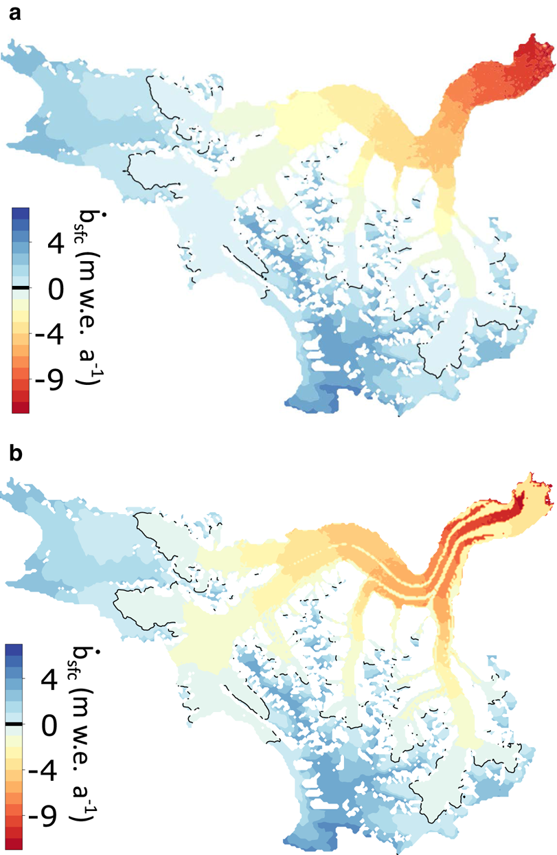
Fig. 7. Mass-balance model results. (a) Reference mass-balance field for debris-free case. (b) Same as in (a) but for debris-present case.
Uncertainty on the modelled glacier-wide mass balance arises from uncertainty on the modelled melt and uncertainty on the downscaled and bias-corrected accumulation. For the melt term we use the standard deviation of the modelled melt rates across all 12 or 25 simulations that pass the two-stage tuning as the uncertainty $\delta _{\dot {A}_{\rm sfc}}$ . For the accumulation term, we use the mean absolute differences between modelled and measured values (see ‘Accumulation bias correction’ section), normalised by the measured values, to establish a relative uncertainty that is applied to the downscaled and bias-corrected accumulation rates to obtain a dimensional uncertainty $\delta _{\dot {C}_{\rm sfc}}$
 . We then compute uncertainty on the mass balance as $\delta _{\dot {B}_{\rm sfc}} = \sqrt {\delta _{\dot {A}_{\rm sfc}}^2 + \delta _{\dot {C}_{\rm sfc}}^2 }$
 .
.
Balance fluxes
Volumetric balance fluxes at each of the nine flux gates (Fig. 8a, Table 1) are determined from the modelled mass-balance fields $\dot {b}_{\rm sfc}$ as:
as:

where A is the glacier area upstream of the flux gate of interest. This approach produces 12 and 25 sets of balance fluxes at each gate for debris-present and debris-free cases, respectively. The reference balance fluxes at each flux gate are the averages of these 12 or 25 values. Uncertainty on the balance fluxes is determined directly from uncertainty on the mass-balance field as described above. We also report the standard deviation of the balance fluxes from all 12 or 25 simulations to give a sense of the variability.
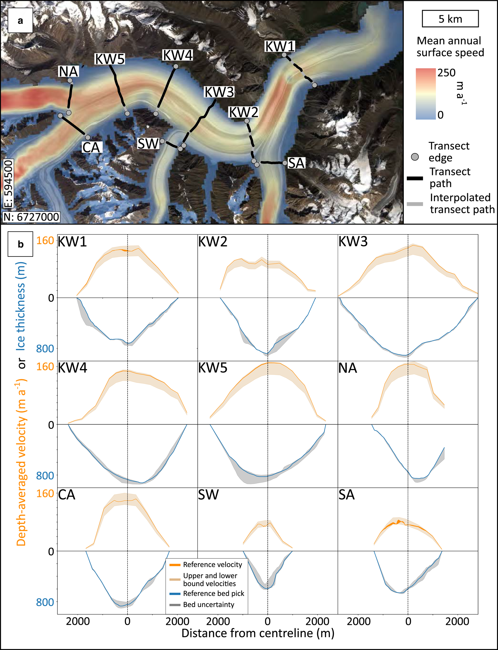
Fig. 8. Observed profiles of ice thickness and depth-averaged velocity. (a) Kaskawulsh Glacier ablation zone with locations of radar transects across the main trunk (KW1–KW5) and across confluences with major tributaries: North Arm (NA), Central Arm (CA), South Arm (SA), Stairway Glacier (SW). Mean 2007–18 surface velocity is shown in colour. Velocity data generated using auto-RIFT (Gardner and others, Reference Gardner2018) and provided by the NASA MEaSUREs ITS_LIVE project (Gardner and others, Reference Gardner, Fahnestock and Scambos2019). UTM (Zone 7 North) coordinates of southwest corner: 594500 E, 6727000 N. Copernicus Sentinel data 2017. Retrieved from Copernicus Open Access Hub 01/11/17. (b) Depth-averaged velocity profiles with uncertainty (orange) and ice-thickness profiles with uncertainty (blue) at each transect.
Table 1. Balance fluxes Q bal, standard deviations σQ and uncertainties δQ at each flux gate (refer to Fig. 8) for debris-present and debris-free cases.

Tributary flux gates are: North Arm (NA), Central Arm (CA), Stairway Glacier (SW), South Arm (SA). Flux gates along the main trunk are: KW5 (highest) to KW1 (lowest). All values in km3 a−1.
For both debris-free and debris-present cases, balance fluxes are greatest somewhere downstream of the North and Central Arm tributaries and decrease thereafter towards the terminus (Table 1). The primary differences between balance fluxes derived from the debris-free vs debris-present cases are: (1) the debris-free balance fluxes are consistently higher and (2) negative balance fluxes extend farther upstream (to KW2) for the debris-present case. Negative balance fluxes indicate that a glacier is out of balance and losing mass, and highlight areas where glacier presence is unsustainable under a given mass-balance regime.
Sensitivity analysis
Here, we quantify the sensitivity of the modelled mass balance to (1) the temperature and accumulation bias corrections, (2) the rain-to-snow temperature threshold and (3) refreezing. We determine the sensitivity of the model to each of these components by comparing the glacier-wide mass-balance rate $\dot {B}_{\rm sfc}$ computed from the mean $\dot {b}_{\rm sfc}$
 fields (using the 25 and 12 parameter combinations for debris-free and debris-present cases, respectively) and resulting balance fluxes when each model component is disabled (bias corrections and refreezing) or changed (rain-to-snow threshold) (Table 2 and Supplementary material). Model components are disabled/changed independently, thus we do not evaluate their interdependence. Changes in $\dot {B}_{\rm sfc}$
 are similar for both debris-free and debris-present simulations, except in the case of the temperature bias correction.
Table 2. Sensitivity of glacier-wide mass balance (m w.e. a−1) for debris-free and debris-present cases to: disabling temperature bias correction (No ΔT), disabling accumulation bias correction (No ΔC), disabling refreezing parameterisation (No RF) and changing rain-to-snow threshold temperature (T R2S).
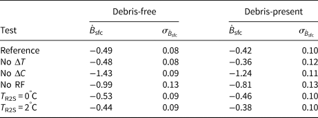
For each test and the reference runs, glacier-wide mass balance $\dot {B}_{\rm sfc}$ and standard deviation $\sigma _{\dot {B}_{\rm sfc}}$
 are given in m w.e. a−1.
Accumulation bias correction
Disabling the accumulation bias correction triples the mass loss (decreasing $\dot {B}_{\rm sfc}$ ), the largest response of all sensitivity tests. The resulting balance fluxes are negative at all gates due to the strong elevation dependence of the accumulation bias correction, including the marked increase in ΔC at elevations >2300 m a.s.l. (Fig. 5b). With 52% of the glacier area above 2300 m a.s.l. (Fig. 5c), the bias correction produces accumulation increases of 2–5 times over a significant area. The gap between measured and downscaled NARR accumulation speaks to the necessity of applying a bias correction. However, it is important to note that the high-elevation data used for this bias correction come from the western margin of the catchment (North/Central Arms), rather than the southern margin (Stairway Glacier/South Arm) where much of the high-elevation terrain is found. The bias correction is thus unconstrained in the area where it has the largest impact, and its effects must therefore be interpreted with caution.
Temperature bias correction
Disabling the temperature bias correction increases $\dot {B}_{\rm sfc}$ by < 0.01 m w.e. a−1 and 0.06 m w.e. a−1 for the debris-free and debris-present cases, respectively (with correspondingly small changes to balance fluxes). This small change in $\dot {B}_{\rm sfc}$
 is the result of averaging positive and negative anomalies arising from the 25 debris-free cases, and mostly positive but small anomalies for the 12 debris-present cases. The temperature bias correction results in modest increases in mid-April to mid-August temperatures, but marked to drastic decreases in temperatures during the rest of the year (Fig. 4b). Therefore, with the bias correction applied, PDDs increase during much of the melt season but decline in the shoulder seasons. Accumulation is also affected via the rain-to-snow threshold temperature, with less accumulation from mid-April to mid-August but more otherwise. Overall, the model sensitivity to temperature bias correction is minimal, producing an order of magnitude lower impact on $\dot {B}_{\rm sfc}$
 compared with disabling the accumulation bias correction or refreezing.
Refreezing model and rain-to-snow threshold
Disabling the refreezing parameterisation causes an earlier seasonal transition from snow to ice, and thus an increase in melt owing in part to the higher radiation factors for ice compared to snow (a ice/snow), resulting in an approximate doubling of mass loss. Disabling refreezing also increases the frequency and intensity of mid-winter melt events caused by positive temperatures, in some cases depleting the snowpack entirely and exposing the underlying ice. The widespread nature of these modelled mid-winter ablation events that occur when refreezing is disabled are considered unrealistic. We also test the model sensitivity to rain-to-snow thresholds of 0 and 2°C, bracketing the reference value of 1°C. These values produce variations in modelled $\dot {B}_{\rm sfc}\lt \! \pm 0.05$ m w.e. a−1 for both debris-free and debris-present cases.
Ice fluxes
We use new IPR data, along with the NASA MEaSUREs ITS_LIVE surface velocities (Gardner and others, Reference Gardner, Fahnestock and Scambos2019), to estimate the observed 2007–18 ice fluxes at nine gates in the ablation area of Kaskawulsh Glacier. The flux gates (Fig. 8a) are roughly perpendicular to the direction of ice flow, with five spanning the main trunk of the glacier and four spanning the major tributaries (North Arm, Central Arm, Stairway Glacier, South Arm). Ice-flux estimates are confined to the ablation area by the radar-data coverage. We compare the observed fluxes to balance fluxes at the same locations obtained using the modelled surface mass balance described above. Below we describe the determination of glacier cross-sectional area based on collection, processing and interpretation of IPR data, followed by the estimation of depth-averaged velocities using the NASA MEaSUREs ITS_LIVE surface-velocity dataset.
Flux-gate geometry
IPR data collection
Ground-based IPR data were collected in 2018 and 2019 with a ruggedised BSI IceRadar system (Mingo and Flowers, Reference Mingo and Flowers2010; Mingo and others, Reference Mingo, Flowers, Crawford, Mueller and Bigelow2020), comprising a Narod and Clarke (Reference Narod and Clarke1994) impulse transmitter (from Bennest Enterprises Ltd.) with a ± 600 V pulse and a pulse repetition frequency of 512 MHz. The receiving unit employs a 12-bit digitiser (Pico 4227), an integrated single-frequency global positioning system (GPS) unit (Garmin NMEA GPS18x) and Blue Systems Integrated IceRadar Acquisition Software. The GPS unit is used only to obtain horizontal coordinates. Receiver and transmitter are connected to identical sets of resistively loaded dipole antennas of 5 MHz centre frequency which were towed in-line at ~30 m separation during the common-offset surveys. During data acquisition, we collected 1024 stacks every 2–3 s at walking speed. The IPR surveys traversed debris-free and debris-covered ice, including some of the prominent medial moraines. Minor detours were required to navigate supraglacial streams, while data gaps within and at the ends of some transects arose from unnavigable terrain. In total, ~30 line-km of data were collected.
IPR data processing and interpretation
Gain control and band-pass filtering were applied to all radar data, following the processing workflow that we have established for ice-depth determination using this radar system in the same environmental setting (Wilson, Reference Wilson2012; Wilson and others, Reference Wilson, Flowers and Mingo2013; Bigelow, Reference Bigelow2019; Bigelow and others, Reference Bigelow2020). We tested 2-D frequency–wavenumber migration on all transects and considered results where migration did not introduce clearly implausible features. Two-way traveltimes were converted to depth considering receiver–transmitter separation and assuming a radar wave velocity of 1.68 × 10⁸ m s−1 (Bogorodsky and others, Reference Bogorodsky, Bentley and Gudmandsen1985). The bed reflector was evident and unambiguous across most or all of the transect length for five of nine transects, while four of nine had larger areas of ambiguity. These areas were sometimes associated with the deepest ice (approaching ~1000 m), and other times with clutter and/or scattering that would have obscured reflections.
In this study, uncertainty in ice depth arises from: (a) inherent uncertainty associated with signal wavelength, (b) the assumed radar velocity, (c) possible near-bed off-nadir reflections transverse to the survey direction, (d) visibility and/or ambiguity of the bed reflector, (e) choices in data processing steps and (f) data gaps. Sources (d)–(f) are expected to dominate (a)–(c) in this study. To acknowledge these uncertainties, we identify minimum and maximum bounds on ice depth by producing a range of ice-depth profiles; we also produce a reference profile, which we subjectively deem most plausible. The range of depth profiles arises from picking different reflectors, where they exist, to address (c) and (d), considering migrated and unmigrated data to address (e) and employing linear vs non-linear interpolation schemes to fill gaps between transect segments and between transect endpoints and glacier margins to address (f). At least six and up to 12 different ice-depth profiles were generated for each transect. The minimum, maximum and reference ice-depth profiles are shown in Figure 8. In order of importance, the depth uncertainty imparted by (d) > (e) > (f), yet the sum of these uncertainties (± in Table 3) is a minor contributor to ice-flux uncertainty (Q high − Q low in Table 3), which includes uncertainty in the velocity–depth profile.
Table 3. Measured cross-sectional area A xc (km2) and ice discharge Q (km3 a−1) at flux gates.

Q (km3 a−1) is derived from cross-sectional area and ITS_LIVE surface velocities for three different velocity–depth profiles: (1) all deformation, no sliding: $\overline {u} = \overline {u}_{\rm d}$ , u b = 0 (Q low); (2) all sliding, no deformation (plug flow): $\overline {u} = u_{\rm b}$
 , u d = 0 (Q high); (3) deformation and sliding combined: $\overline {u} = \overline {u}_{\rm d} + u_{\rm b}$
 (Q ref). Tributary flux gates are: North Arm (NA), Central Arm (CA), Stairway Glacier (SW), South Arm (SA). Flux gates along the main trunk are: KW5 (highest) to KW1 (lowest). ± indicates one standard deviation arising from bed interpretation for A xc and variations in bed interpretation only for the fluxes. Bold values are explained in text.
Depth-averaged velocities
At each transect, cross-glacier depth-averaged velocity profiles (i.e. $\bar {u}\lpar y\rpar$ ) are generated using surface-velocity data and assumptions about flow partitioning between sliding and deformation. Surface velocities are obtained from the NASA MEaSUREs Inter-Mission Time Series of Land Ice Velocity and Elevation (ITS_LIVE) project (Gardner and others, Reference Gardner, Fahnestock and Scambos2019). These data are generated using Landsat 4, 5, 7 and 8 imagery and auto-RIFT feature tracking (Gardner and others, Reference Gardner2018) to produce annual velocity mosaics. At each of our flux gates, we extract annual surface velocity profiles from the 240 m×240 m gridded ITS_LIVE dataset for the 2007–18 study period.
From the 2007–18 profiles we compute a 12-year mean velocity profile at each transect (Fig. 8). We consider three velocity models, which respectively give rise to lower, higher and intermediate estimates of depth-averaged velocity $\overline {u}$ : (a) all deformation (u d), no basal sliding (u b): $\overline {u} = \overline {u}_{\rm d}$
 , u b = 0; (b) all basal sliding, no deformation (plug flow): $\overline {u} = u_{\rm b}$
 , u d = 0; and (c) some combination of deformation and basal sliding: $\overline {u} = \overline {u}_{\rm d} + u_{\rm b}$
 . In (a) we take $\overline {u}_{\rm d} = 0.8 \, u_{\rm s}$
 , where u s is the surface velocity (Nye, Reference Nye1965), thus $\overline {u} = 0.8 \, u_{\rm s}$
 . In (b) $\overline {u} = u_{\rm s}$
 . In (c), we estimate the contribution of deformation to surface velocity using the shallow ice approximation, up to a maximum of the observed surface velocity:

with A = 2.4 × 10⁻²⁴ Pa−3 s−1 the assumed value of the flow-law coefficient for temperate ice (Cuffey and Paterson, Reference Cuffey and Paterson2010), n = 3 the flow-law exponent, ρ i = 910 kg m−3 the density of ice, g = 9.81 m s−2 the acceleration due to gravity, h the ice depth and θ the glacier surface slope. For each transect, we estimate θ as the width-averaged surface slope in the downflow direction based on the TanDEM-X DEM.
Any underestimation of the observed surface velocity by the value calculated in Eqn (8) is attributed to basal sliding: u b = u s − u d(z = s). The depth-averaged velocity is then $\overline {u} = 0.8 \, {u}_{\rm d}\lpar z = s\rpar + u_{\rm b}$ or $\overline {u} = u_{\rm s} - 0.2 \, {u}_{\rm d}\lpar z = s\rpar$
 . The choice of velocity model is the leading source of uncertainty in the ice-flux calculations.
Observed ice fluxes
Ice-flux (in units of km3 a−1) is calculated at each flux gate (i.e. transect) by numerically integrating the product of ice depth (derived from radar data) and depth-averaged velocity (derived from ITS_LIVE data) across the transect (i.e. glacier width). This calculation is done for each of the 6–12 ice-depth profiles per transect and each of the three depth-averaged velocity models above, yielding 18–36 values of ice flux per transect. The reference flux at each transect employs the reference ice-depth profile, and the intermediate velocity model (c), where the shallow-ice approximation is used to estimate the contribution of deformation to the surface velocity (Eqn (8)) and the remainder is attributed to sliding. We assign an uncertainty on each ice flux in Table 3 (Q low, Q high, Q ref) equal to the standard deviation of the 6–12 values. This uncertainty represents only that arising from bed interpretation, whereas the range of Q low to Q high encompasses the uncertainty arising from different velocity models.
Analysis and interpretation
Comparison of modelled and continuity-derived mass-balance distribution
Using the surface elevation change of the Kaskawulsh Glacier (Fig. 2), the ice fluxes at each of nine flux gates (Fig. 8) and the modelled surface mass balance (Fig. 7), we are able to independently estimate each term in the continuity equation:

where ∂h/∂t is the local rate of change of ice thickness (obtained from geodetic mass balance), $\nabla \cdot q$ is the divergence of the flux (computed from ITS_LIVE surface velocities and IPR-derived ice thicknesses) and $\dot {b}_{\rm sfc}$
 is the surface mass balance (modelled using downscaled reanalysis products). Densities of 850 and 900 kg m−3 have been used to convert ∂h/∂t and $\nabla \cdot q$
 , respectively, into units of m w.e. a−1. In order to test our remotely sensed elevation changes, measured ice fluxes and modelled mass balance against mass continuity, we compare each independently estimated term in the continuity equation to its counterpart calculated using the other terms, for each section of the glacier bounded by flux gates and the ice margin.
We then compute the RMSE between the two estimates of each term for each section of the glacier for both debris-free and debris-present cases of the mass-balance model. Inspection of the RMSEs reveals that the debris-present case outperforms the debris-free case for each term in the continuity equation: 1.43 vs 1.61 m w.e. a−1 for ∂h/∂t, 0.58 vs 0.70 m w.e. a−1 for $\nabla \cdot q$ and 1.31 vs 1.47 m w.e. a−1 for $\dot {B}_{\rm sfc}$
 . The debris-present case also outperforms the debris-free case using mean error rather than RMSE as a metric. We therefore consider $\dot {b}_{\rm sfc}$
 obtained with the debris-present model to be the reference mass-balance field in the following analysis. Although the spatial pattern associated with debris-covered medial moraines in the mass-balance model (Fig. 7b) is not clearly reflected in the observed surface lowering (Fig. 2), the superior performance of the model with debris is nevertheless unsurprising: muted thinning rates over the lowermost ~5 km of the glacier (Fig. 2) do coincide with extensive debris cover. Furthermore, the ablation suppressed by debris in the model is compensated by enhanced ablation over debris-free ice owing to the requirement (in Stage 1 tuning) that modelled glacier-wide mass balance match the geodetic balance within uncertainty; the resulting model parameters (MF, a snow/ice) for the debris-present case yield a lower modelled mass-balance gradient, which is in better agreement with the observations. A similar dependence of the mass-balance gradient on debris cover has been observed on glaciers in High Mountain Asia (Bisset and others, Reference Bisset2020).
By using ice-thickness data collected in 2018–19, we systematically underestimate 2007–18 mean ice fluxes due to thinning during the study period. In order to assess the maximum impact of this underestimation on $\nabla \cdot q_{\rm obs}$ , we use the observed elevation change (data in Fig. 2) to calculate total thinning at each flux gate between 2007 and 2018. Note that gap-filled areas comprise up to 53% (KW2) of the length of individual flux gates. This calculation yields an average change in $\nabla \cdot q_{\rm obs}$
 of ~1.5 ± 1.2%, with the greatest change between KW4 and KW5 (~4%) and least between KW1–KW2 (<1%). These values reflect flux changes over the entire study period, and are thus twice what might be considered representative of the 2007–18 mean.
Below we focus on the comparison between modelled ($\dot {B}_{\rm mod}$ ) and calculated ($\dot {B}_{\rm cal}$
 ) mass balance for each section of the glacier bounded by flux gates and the glacier margin, where $\dot {B}_{\rm mod}$
 is the integral of $\dot {b}_{\rm sfc}$
 between the flux gates of interest and $\dot {b}_{\rm sfc}$
 is obtained directly from the mass-balance model with debris. $\dot {B}_{\rm cal}$
 is obtained by summing the elevation change (∂h/∂t) over the section of interest and the difference in measured downstream and upstream fluxes ($\nabla \cdot q$
 ) (Eqn (9)). This comparison is one means of evaluating the mass-balance model, but also reveals potential shortcomings in the other derived quantities.
Sections upstream of tributary flux gates
Values of $\dot {B}_{\rm mod}$ are positive for all four tributaries (NA, CA, SW, SA in Fig. 9) but underestimate $\dot {B}_{\rm cal}$
 for North and Central Arms, while overestimating $\dot {B}_{\rm cal}$
 for Stairway Glacier and South Arm. $\dot {B}_{\rm cal}$
 for Stairway Glacier (the smallest of the four catchments) is near-zero and for South Arm is negative. $\dot {B}_{\rm mod}$
 and $\dot {B}_{\rm cal}$
 agree within uncertainty only for the North and Central Arms. Averaged across all four tributaries, B mod exceeds B cal by 0.16 m w.e.
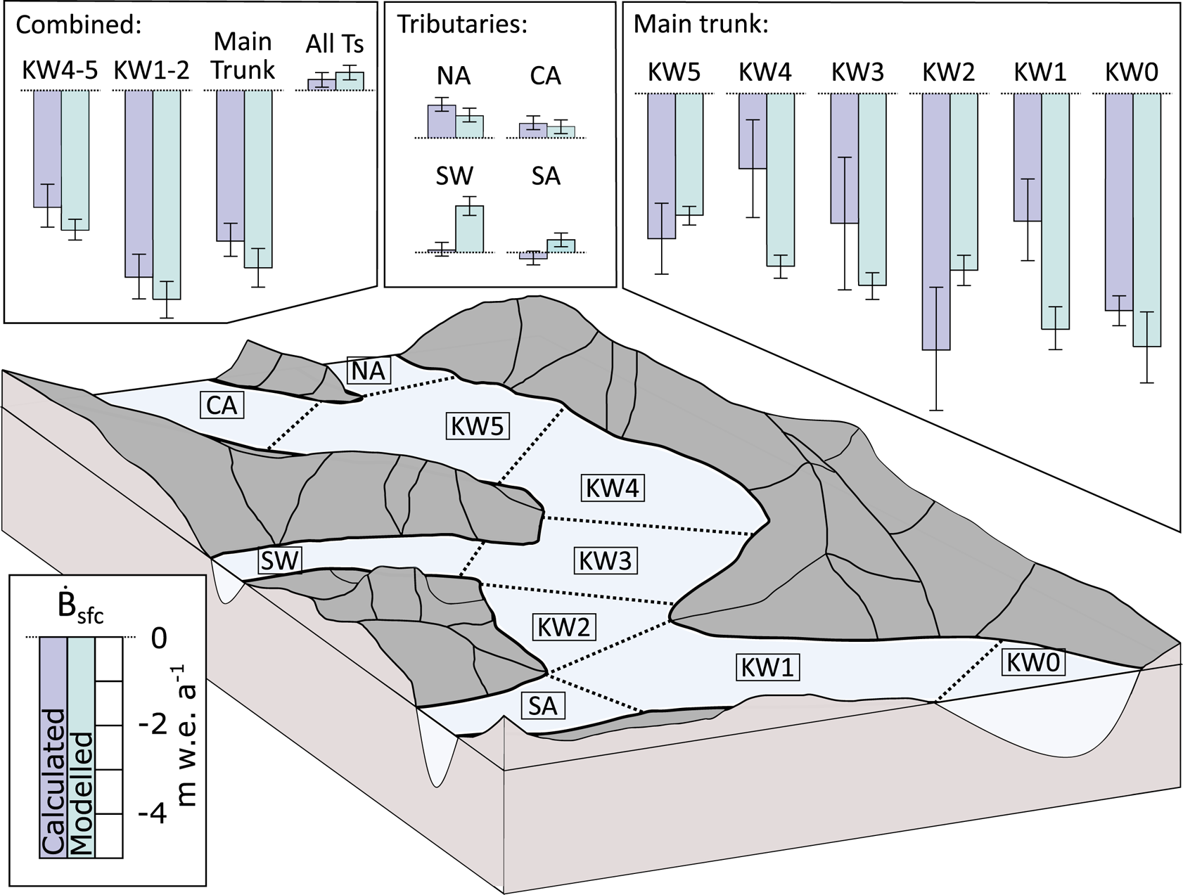
Fig. 9. Comparison of calculated ($\dot {B}_{\rm cal}$ , light purple) and modelled ($\dot {B}_{\rm mod}$
 , light blue) mass balance, with associated uncertainties, for each section of the glacier. Sections are labelled according to their downstream flux gates. Also shown are four combined sections: KW4 and KW5 (‘KW4–5’); KW1 and KW2 (‘KW1–2’); KW0 through KW5 (‘Main trunk’); and NA, CA, SW, SA (‘All Ts’ for all tributaries).
The differences between $\dot {B}_{\rm mod}$ and $\dot {B}_{\rm cal}$
 hint that spatial variability in the accumulation field not captured by the model might play an important role in explaining this mismatch, and in Kaskawulsh Glacier mass balance. The better agreement between $\dot {B}_{\rm mod}$
 and $\dot {B}_{\rm cal}$
 in the North and Central Arms is unsurprising given the provenance of the high-elevation measurements used in the accumulation bias correction (Fig. 5). A strong roughly east–west moisture gradient exists in the region due to the orographic divide of the St. Elias Mountains: applying a bias correction exclusively based on elevation and without data from the southern half of the catchment (the accumulation areas of Stairway Glacier and South Arm) would not account for geographic differences in accumulation. Given that Stairway Glacier and South Arm are further from the orographic divide, we suspect the accumulation bias correction – based on high-elevation data restricted to the western margin of the catchment – leads to overestimation of modelled mass balance in these southern tributary catchments. The North and Central Arms also differ from Stairway Glacier and South Arm in aspect, with the former being easterly to north-easterly and the latter being northerly. Aspect plays a direct role in modelled ablation through parameters a snow/ice, while the orientation of mountain ridges relative to the prevailing wind would also play a role in snow redistribution, a process unaccounted for in the model.
Sections downstream of the tributary flux gates
Within the main trunk of the glacier, we compare $\dot {B}_{\rm mod}$ and $\dot {B}_{\rm cal}$
 for six sections bounded by the flux gates and the glacier margin/terminus. The differences between $\dot {B}_{\rm mod}$
 and $\dot {B}_{\rm cal}$
 are large and their signs inconsistent (Fig. 9): $\dot {B}_{\rm mod}$
 exceeds $\dot {B}_{\rm cal}$
 by 2.15, 1.33, 2.34 and 0.80 m w.e. (127, 45, 79 and 17%) for sections upstream of KW4, KW3, KW1 and the terminus, respectively, while $\dot {B}_{\rm cal}$
 exceeds $\dot {B}_{\rm mod}$
 by 0.58 m w.e. and 1.89 m w.e. (21 and 49%) upstream of KW5 and KW2, respectively. $\dot {B}_{\rm mod}$
 and $\dot {B}_{\rm cal}$
 only agree within uncertainty for three of six sections. Notably, in the lowermost section between KW1 and the terminus (labelled KW0) where the debris coverage is highest, the debris-present model far outperforms the debris-free model, yielding $\dot {B}_{\rm mod} = -5.62 \pm 0.46$
 m w.e. vs −9.64 ± 0.99 m w.e. for the debris-free model, compared to $\dot {B}_{\rm cal} = -4.82 \pm 0.16$
 m w.e. The magnitude of this difference is in line with the reduction of ablation by terminus debris cover observed in High Mountain Asia (e.g. Vincent and others, Reference Vincent2016; Bisset and others, Reference Bisset2020).
Visual inspection of Figure 9 reveals changes in the sign of the mismatch between $\dot {B}_{\rm mod}$ and $\dot {B}_{\rm cal}$
 in some adjacent sections of the glacier, suggesting that mismatch could be reduced by combining these sections. For example, if we combine sections KW4 and KW5, $\dot {B}_{\rm mod}$
 and $\dot {B}_{\rm cal}$
 differ by only 22% (Fig. 9, Table 4). Similarly, KW1 and KW2 together reduce the mismatch between $\dot {B}_{\rm mod}$
 and $\dot {B}_{\rm cal}$
 to 11%. Considering the entire region below the tributary fluxgates, $\dot {B}_{\rm mod}$
 is more negative than $\dot {B}_{\rm cal}$
 (−4.01 vs −3.41 m w.e.), whereas above the tributary flux gates $\dot {B}_{\rm mod}$
 is more positive (0.41 vs 0.25 m w.e.) (Fig. 9, Table 4). The modelled mass-balance gradient is therefore steeper than that inferred from $\partial h/\partial t + \nabla \cdot q$
 .
.
Table 4. Independently estimated (subscript ‘obs’ or ‘mod’) vs calculated (subscript ‘cal’) terms in the continuity equation (Eqn (9)) for each section of the glacier (labelled with downstream flux gate as in Fig. 9): ${\partial h\over \partial t}_{\rm cal} = -\nabla \cdot q_{\rm obs} + \dot {B}_{\rm mod}$ , $\dot {B}_{\rm cal} = {\partial h\over \partial t}_{\rm obs} + \nabla \cdot q_{\rm obs}$
 , $\nabla \cdot q_{\rm cal} = \dot {B}_{\rm mod} - {\partial h\over \partial t}_{\rm obs}$

Values of $\nabla \cdot q$ are converted to m w.e. a−1 using an ice density of 900 kg m−3.
Missing physical processes can also explain some of the mismatch between $\dot {B}_{\rm mod}$ and $\dot {B}_{\rm cal}$
 . For example, the section above KW5 is influenced by the presence of an ice-marginal lake with a calving front (Bigelow and others, Reference Bigelow2020), which results in additional mass loss. This loss is not accounted for in the mass-balance model, but nevertheless influences changes in surface elevation and ice flux. Though unquantified, the anticipated mass loss into the lake basin is consistent with the sign of the mismatch between $\dot {B}_{\rm mod}$
 and $\dot {B}_{\rm cal}$
 above the KW5 flux gate.
Discrepancies between $\dot {B}_{\rm mod}$ and $\dot {B}_{\rm cal}$
 can also be due to observational errors or uncertainty that influence $\dot {B}_{\rm cal}$
 , in addition to shortcomings of the mass-balance model. Occurrence of cloud cover or the presence of regions where stereo-image texture is too homogeneous creates the need to gap-fill the observed elevation-change field (∂h/∂t in Eqn (9)). These gaps could contribute to mismatch between ∂h/∂t cal and ∂h/∂t obs: 27.7% of the total glacier area is gap-filled (Fig. 2), with a local maximum of 48.7% for the section upstream of KW2 (Table 4). Because the gap-filling scheme is a function of elevation only, it does not capture small-scale spatial variability associated with debris cover, aspect or geographical location within the catchment (McNabb and others, Reference McNabb, Nuth, Kääb and Girod2019). This is problematic in higher elevations terrain, which occupies a wide geographical range and has variable aspects. Compounded with larger relative errors at high elevation (owing to smaller values of elevation change), we expect the gap-filled values at high elevations may be less representative of local conditions.
Errors also arise in the calculation of ice fluxes. There are three major sources of uncertainty in our calculation: that associated with (1) ice depth, due to processing and interpretation of the radar data, (2) surface velocity, arising from inter-annual variability evident in the ITS_LIVE data and (3) the velocity-depth profile, owing to the unknown partitioning of surface velocity between deformation and sliding. The latter is the largest. Inconsistency also arises from using radar data collected in 2018–19 to compute 2007–18 fluxes, given the nearly pervasive thinning observed from 2007 to 2018 (Fig. 2).
Entertaining the possibility that Q ref (Table 3) may not be the correct representation of flux at each gate, we explore the impact of substituting Q low ± σ (no sliding) and Q high ± σ (plug flow) for Q ref. By increasing the sliding contribution at gates SW, SA and KW2, and decreasing it at gates NA, KW4, KW3 and KW1 (see bold values in Table 3), we reduce metrics of overall mismatch between $\nabla \cdot q_{\rm obs}$ and $\nabla \cdot q_{\rm cal}$
 (Table 4) by ~20–40% and section-wise mismatch of $\nabla \cdot q_{\rm obs}$
 and $\nabla \cdot q_{\rm cal}$
 downstream of the tributary flux gates from >75 to <25% (not shown). The resulting mismatch between $\dot {B}_{\rm cal}$
 and $\dot {B}_{\rm mod}$
 is more systematic and spatially coherent than that using Q ref in Figure 9, particularly below the tributary flux gates (not shown). With one minor exception, $\dot {B}_{\rm cal}$
 underestimates the magnitude of $\dot {B}_{\rm mod}$
 by 11–24% for KW0–KW5 ($\dot {B}_{\rm cal}$
 overestimates the magnitude of $\dot {B}_{\rm mod}$
 by 9% for KW4). Although it would be circular to tune $\dot {B}_{\rm cal}$
 to $\dot {B}_{\rm mod}$
 by changing the fluxes, this exercise demonstrates that it is possible to satisfy the local continuity equation simply by exploring plausible variations in glacier dynamics via the partitioning of sliding and deformation. It also corroborates our finding that the modelled mass-balance gradient is steeper than that inferred from $\partial h/\partial t + \nabla \cdot q$
 .
.
Comparison of balance fluxes and observed fluxes
We compare our model-derived balance fluxes (Q bal) and observed fluxes (Q obs) at each flux gate to investigate the imbalance between internal mass redistribution and surface mass balance of the Kaskawulsh Glacier (Fig. 10). First, we determine two sets of balance fluxes: (1) those derived from the 2007–18 modelled mass balance where $\dot {B}_{\rm sfc} = -0.42$ m w.e. a−1 (denoted $Q_{{\rm bal}_{-0.42}}$
 ), and (2) those adjusted to balance conditions ($\dot {B}_{\rm sfc} = 0$
 ) (e.g. Azam and others, Reference Azam2012) by adding −0.42 m w.e. a−1 to the b sfc field (denoted $Q_{{\rm bal}_{0}}$
 ). The contrast between these balance fluxes is used to situate the current state of response of the observed ice fluxes to the surface mass balance.

Fig. 10. Comparison of observed and balance fluxes arranged according to position of flux gate (tributaries shaded in grey). See Figure 8 for flux-gate locations. Observed fluxes (Q obs, yellow) are shown with standard deviations arising only from glacier-bed interpretation (see Q ref in Table 3). Balance fluxes are shown for $\dot {B}_{\rm sfc} = 0$ ($Q_{{\rm bal}_{0}}$
 , blue) and $\dot {B}_{\rm sfc} = -$
 0.42 m w.e. ($Q_{{\rm bal}_{-0.42}}$
 , red). Dark red/blue shading is standard deviation of balance fluxes for the 12 simulations that satisfy both stages of model tuning for debris-present case. Light red/blue shading is the uncertainty for each balance flux determined from the uncertainties on model accumulation and melt rates. Shading is continuous between flux gates only to assist in visual interpretation; not all flux gates are connected as suggested by shading.
With the exception of the SW and SA flux gates, where the balance fluxes are impacted by the suspected overestimation of modelled accumulation, the spatial structure of Q obs resembles that of $Q_{{\rm bal}_{0}}$ (Fig. 10). The magnitudes of Q obs are lower than those of $Q_{{\rm bal}_{0}}$
 , but significantly higher than those of $Q_{{\rm bal}_{-0.42}}$
 . The similarity in distribution and magnitude of Q obs and $Q_{{\rm bal}_{0}}$
 indicates that the glacier flow regime more closely reflects zero balance conditions than the negative balance conditions of 2007–18, and thus the dynamic adjustment of the glacier is far from complete. This state of adjustment demonstrates that the response time of the Kaskawulsh Glacier exceeds the ~40 years over which mass-balance conditions have been characterised by sustained, cumulative mass-loss similar to those of 2007–18 (Berthier and others, Reference Berthier, Schiefer, Clarke, Menounos and Rémy2010), as expected for a glacier of this size and in this climate (Cuffey and Paterson, Reference Cuffey and Paterson2010).
The balance flux $Q_{{\rm bal}_{-0.42}}$ becomes negative between gates KW3 and KW2 (Fig. 10). Owing to the suspected overestimation of accumulation in the SW and SA tributaries, which feed downstream gates KW3 and KW1, respectively, the spatial extent of negative balance fluxes is likely a conservative estimate. In order to more precisely determine the position of zero balance flux (KWnull), we discretise the region between KW3 and KW2 into numerous flux gates and integrate the modelled surface mass-balance upstream of each one. We estimate KWnull to be 23.2 ± 3.2 km upstream of the current terminus position, and upstream of the South Arm confluence, at an elevation of 1447 m a.s.l (Fig. 1). This position suggests the main trunk of the Kaskawulsh Glacier would detach from the South Arm under sustained conditions of 2007–18 mass balance. Using a slightly adjusted (Langhammer and others, Reference Langhammer, Grab, Bauder and Maurer2019) version of the Farinotti and others (Reference Farinotti2019) ensemble estimate of glacier bed topography, we estimate that 46 km3 of ice, or ~15% of the total Kaskawulsh Glacier volume, reside in the main trunk of the glacier below the position of zero balance flux. Given that our calculation ignores flow across the line of zero balance as well as upstream thinning and the mass-balance–elevation feedback, this volume is a minimum bound on the committed ice loss (Mernild and others, Reference Mernild, Lipscomb, Bahr, Radić and Zemp2013) if the 2007–18 climate persists. Considering the projected increase of global and regional air temperatures (IPCC, Reference Pachauri and Meyer2014) compared to our model inputs, the negative mass-balance conditions that characterised 2007–18 will likely be exacerbated in the future and drive the position of zero balance flux even further up-glacier.
Discussion
The rate of mass loss we estimate for 2007–18 (−0.46 ± 0.17 m w.e. a−1) is higher than that estimated by Larsen and others (Reference Larsen2015) for 1995–2013 (−0.35 m w.e. a−1), the only other glacier-wide study. Our 2007–18 estimate is, however, indistinguishable from that of Berthier and others (Reference Berthier, Schiefer, Clarke, Menounos and Rémy2010), both for the Kaskawulsh Glacier individually (−0.46 ± 0.20 m w.e. a−1, 1977–2007) and the entire glacier population of the St. Elias Mountains (−0.47 ± 0.09 m w.e. a−1, 1968–2006). Although mass loss may have accelerated from 1995 to 2018, we cannot conclude that it accelerated in the last decade (2007–18) relative to the four before (1968–2006).
Mass loss occurs in two modes for land-terminating glaciers (e.g. Thomson and others, Reference Thomson, Zemp, Copland, Cogley and Ecclestone2017): (1) ice fluxes in excess of balance fluxes move mass to lower ablation-prone areas causing upstream thinning (and an attendant reduction in driving stress) without significant terminus retreat, and (2) reduced ice fluxes lead to accelerated thinning in the mass-starved ablation-prone areas (e.g. Span and Kuhn, Reference Span and Kuhn2003) and eventually to glacier retreat. Previous study on small alpine glaciers (≤ 30 km2) has documented both significantly reduced ice fluxes and accelerated thinning within a decade of decreasing surface mass balance (e.g. Azam and others, Reference Azam2012; Berthier and Vincent, Reference Berthier and Vincent2012; Dehecq and others, Reference Dehecq2019). This ice-flux reduction can overshoot the mass balance forcing even for very small glaciers, resulting in balance fluxes greater than observed fluxes (Meier and Tangborn, Reference Meier and Tangborn1965). The dynamic response can be further complicated by frontal ablation for marine terminating glaciers (Deschamps-Berger and others, Reference Deschamps-Berger2019), variation in surface debris (e.g. Benn and others, Reference Benn2012; Bhattacharya and others, Reference Bhattacharya2016) and glacier geometry (encompassing area/volume, and hypsometry) (e.g. Chinn, Reference Chinn1999). The fact that observed fluxes for the Kaskawulsh Glacier (Q obs) are more in line with balance fluxes adjusted to zero-balance conditions ($Q_{{\rm bal}_{0}}$ vs $Q_{{\rm bal}_{-0.42}}$
 ) suggests that driving stresses have not diminished appreciably. Indeed there is no clear evidence of a systematic decline in surface velocity between 2007 and 2018 (see Supplementary material), consistent with Mode 1 (see above) mass loss. However, the elevation-dependent thinning observed (Fig. 2) suggests the Kaskawulsh Glacier also exhibits some aspects of mass loss consistent with Mode 2.
Based on the position of the zero balance flux ($Q_{{\rm bal}_{-0.42}} = 0$ ), we calculate a minimum of ~23 km of committed glacier retreat if the 2007–18 climate were to hold steady. Although we cannot assign a timescale to this retreat, Foy and others (Reference Foy, Copland, Zdanowicz, Demuth and Hopkinson2011) have determined a rate of terminus retreat of ~13 m a−1 (derived from terminus tracking between 1956 and 2007 using aerial and satellite imagery) that increased between 2000 and 2007. Reyes and others (Reference Reyes, Luckman, Smith, Clague and Van Dorp2006) estimate a late Holocene retreat rate of ~80–100 m a−1 based on dendroglaciological studies of the Little Ice Age (LIA) maximum. Due to the onset of Kaskawulsh retreat occurring later than the regional LIA maximum (early- to mid-18th century), the estimated retreat rate is likely conservative (Borns and Goldthwait, Reference Borns and Goldthwait1966; Reyes and others, Reference Reyes, Luckman, Smith, Clague and Van Dorp2006). At these historically estimated rates, the committed retreat of ~23 km would occur on timescales of a century or longer.
Our observations of glacier mass loss coincide with an observed multi-decadal increase in regional air temperature (Streicker, Reference Streicker2016) that is projected to continue for decades to come. Yukon has experienced a greater warming rate than most regions in Canada: a 2.4°C increase in mean annual air temperature for 1948–2016 (ECCC, 2019b) compared to ~1.7°C for the entire country (ECCC, 2019b). Relative to the 1980–2000 mean, an additional 2.1–3.3°C warming is expected for Yukon by mid-century (2040–2060) and 2.2–6.4°C by late-century (2080–2100) (Data from Environment and Climate Change Canada) based on representative concentration pathways 2.6 and 8.5, respectively, from the Fifth Assessment Report of Intergovernmental Panel of Climate Change (IPCC). Winter temperature increase is typically double the annual mean (Streicker, Reference Streicker2016; ECCC, Reference ECCC2019a). Total annual precipitation in Yukon has increased by 6% between 1964 and 2014 (Streicker, Reference Streicker2016), with a 12–15% increase projected for mid-century (2040–2060) and 12–35% for late-century (2080–2100) relative to the 1980–2000 mean (Data from Environment and Climate Change Canada), less than has been estimated is required to offset the effects of warming (e.g. De Woul and Hock, Reference De Woul and Hock2005). With the anticipated warming yet to come by 2100, the glacier mass-loss rate and committed retreat we have estimated based on 2007–18 data are lower than should be expected for mid- to late-21st century climate conditions.
Conclusion
This study investigates the mass budget of a large land-terminating glacier extending ~70 km over ~2500 m of elevation, using direct measurements of ice geometry and fully distributed mass-balance modelling. We have combined new measurements of surface-elevation change, observed ice fluxes and modelled surface mass balance to calculate the mass budget of the Kaskawulsh Glacier. We estimate a 2007–18 geodetic balance of −0.46 ± 0.17 m w.e. a−1, comparable to the 1977–2007 estimate for the Kaskawulsh Glacier and the 1968–2006 estimate for the wider region. The rate of mass loss and associated glacier thinning is expected to accelerate with continued warming. In comparing observed ice fluxes to model-derived balance fluxes we estimate a committed terminus retreat of 23.2 ± 3.2 km and a lower bound of 46 km3 of ice loss, corresponding to ~15% of the total glacier volume. This retreat will result in fragmentation of the Kaskawulsh Glacier, with the main trunk retreating past the confluence with the South Arm. We find that measured ice fluxes are closer to balance fluxes adjusted to zero-balance conditions than to 2007–18 balance fluxes, indicating that the glacier is still in the early stages of dynamic adjustment to mass imbalance.
By analysing discrepancies between modelled, observed and derived quantities in the context of the continuity equation, we have identified several key considerations in determining the mass budget of large land-terminating glaciers. (1) The best assumption for determining depth-averaged velocity profiles for the purposes of calculating ice flux may vary spatially. (2) Bias corrections to modelled accumulation may be large and spatially variable, due, for example, to orographic effects. Well-distributed accumulation measurements are needed to characterise the accumulation field. (3) Incorporating processes such as refreezing, and properties such as debris cover, into mass-balance models can impart significant influence on the timing and magnitude of modelled melt. (4) Accounting for the effects of debris cover, especially at lower elevations, can significantly alter the modelled mass-balance gradient.
The mass balance of large and regionally significant glaciers like the Kaskawulsh Glacier remains impractical to measure with in situ methods. We therefore need models like the one employed in this study, forced by spatially distributed glacio-meteorological data (e.g. reanalysis products, AWS timeseries, in situ accumulation and ablation measurements), combined with creative, observationally-driven ways to approach model tuning to characterise changing glacier mass budgets.
Supplementary material
The supplementary material for this article can be found at https://doi.org/10.1017/jog.2020.107.
Data Availability
The Kaskawulsh Glacier outline was obtained from https://www.glims.org/maps/glims, the Nasa ITS_LIVE surface velocities were obtained from https://nsidc.org/apps/itslive/, the NARR data used as input to the mass balance model were obtained from https://www.ncdc.noaa.gov/data-access/model-data/model-datasets/north-american-regional-reanalysis-narr, and the SFU Glaciology Group AWS temperature records are available at https://vault.sfu.ca/index.php/s/Io7LCSrcGuvTmo9. Further data available upon request.
Acknowledgments
Permission to conduct field work was granted by the Kluane First Nation (KFN), Parks Canada and Yukon Government. We are grateful to S. Williams, L. Goodwin and S. Shaw for logistical support, and D. Bigelow, C. Wong (Parks Canada) and U. Fischer for assistance in the field. L. Copland kindly provided temperature data used in the NARR bias corrections. We thank L. Mingo for assistance with interpretation of radar data, A. Adhikari for carrying out snowline picks, A. Morin for performing calculations involving the Farinotti and others (Reference Farinotti2019) dataset and H. Jiskoot for helpful discussions related to model tuning. SPOT6/7 data were obtained thanks to public funds received in the framework of GEOSUD, a project (ANR-10-EQPX-20) of the programme ‘Investissements d'Avenir’ managed by the French National Research Agency. EB acknowledges support from the French Space Agency through the TOSCA and DINAMIS projects. EY, GF and RL are grateful for financial support provided by Polar Knowledge Canada, the Natural Sciences and Engineering Research Council of Canada, Simon Fraser University, the Northern Scientific Training Program and the Polar Continental Shelf Program. We would like to thank two anonymous reviewers for their insightful comments.
Author contributions
GF conceived of the original study and EY/GF co-developed the details. EY developed, tuned and ran the mass-balance model, including all aspects of downloading/pre-processing model inputs, analysing model output and integrating output with observations. EY also supervised Adhikari's work on snowlines. GF and EY carried out the field work. RL processed and interpreted the radar data with guidance from GF and calculated the ice fluxes with EY. EB acquired and processed the elevation-change data. EY led the manuscript preparation, with contributions from GF and EB. All authors contributed to various aspects of the interpretation and edited the manuscript.


 Open access