


1. Introduction
Bare ice is exposed subaerially along the margin of the Greenland Ice Sheet (GrIS) for a period of weeks to months each boreal summer, after the previous year's snowfall has melted entirely (Fahnestock and others, Reference Fahnestock, Bindschadler, Kwok and Jezek1993). This region – the ablation zone – presently includes more than 12% of the ice sheet by surface area (McGrath and others, Reference McGrath, Colgan, Bayou, Muto and Steffen2013). The ablation zone is predicted to expand given continued anthropogenic climate warming, and indeed such an expansion was recently reported and is particularly acute for northern Greenland (Noël and others, Reference Noël, van de Berg, Lhermitte and van den Broeke2019). Given downward advection of ice in the accumulation zone and upward advection in the ablation zone, the oldest subaerially exposed surface of an ice mass is generally found along the ice margin, in the ablation zone of land-terminating ice (Hooke, Reference Hooke2020).
Subaerial exposure of ice from the late Pleistocene epoch was first documented in the ablation zone of the Barnes Ice Cap on Baffin Island by Hooke (Reference Hooke1976). There, Pleistocene ice was distinctly whiter than more recent, bluer Holocene ice. Consistent with ice-core records, the stable oxygen-isotope fractionation ratio (δ18O) of candidate Pleistocene ice was also depleted significantly relative to Holocene ice. For Greenland, between 1985 and 1994 (all years Common Era), Niels Reeh and several collaborators sampled surface ice within the GrIS ablation zone and measured its δ18O value. Their goal was to identify sites with inexpensive access to paleoclimatically distinct ice from the late Pleistocene and Holocene epochs (Reeh and others, Reference Reeh, Oerter and Thomsen2002 and references therein; hereafter R02; Fig. 1). That work resulted in a breakthrough for a bulk sampling of paleo-atmospheres, which has since been exploited regularly in Greenland and elsewhere (e.g. Petrenko and others, Reference Petrenko, Severinghaus, Brook, Reeh and Schaefer2006; Aciego and others, Reference Aciego, Cuffey, Kavanaugh, Morse and Severinghaus2007; Schaefer and others, Reference Schaefer2009; Kurbatov and others, Reference Kurbatov2010), and it also informed correlation of surface-intersecting internal radiostratigraphy with surface-exposed visible stratigraphy (Kjær and others, Reference Kjær2018).

Fig. 1. Map of Greenland identifying all δ18O surface-sampling sites reported by R02, including the subset for which δ18O data are available and the new Hiawatha Glacier site reported by this study. Green site labels denote figure numbers/panels where each site is further examined. Black numbers denote primary ice-sheet drainage systems (Zwally and others, Reference Zwally, Giovinetto, Beckley and Saba2012).
As a result of their sampling campaign, R02 identified a visually distinctive surface stratigraphy along the GrIS margin that enables a broad age classification of exposed ice from the late Pleistocene (~129–11.7 ka, where ‘ka’ means thousands of years ago) and Holocene (11.7–0 ka) epochs. Within the late Pleistocene, this classification includes recent major climate transitions within the Last Glacial Period (LGP; ~115–11.7 ka): the Younger Dryas (YD, 12.8–11.7 ka) stadial, Bølling–Allerød (B–A, 14.7–12.8 ka) interstadial and pre-B-A portion of the LGP (115–14.7 ka) (Rasmussen and others, Reference Rasmussen2006). This surface stratigraphy is due to spatiotemporal variability in several factors, including the dust concentration in subaerially deposited snow at the time of burial, and the rates of downward vertical advection (burial) in the upstream dry snow zone, horizontal ice flow and upward advection (emergence) in the ablation zone (e.g. Bøggild and others, Reference Bøggild, Oerter and Tukiainen1996, Reference Bøggild, Brandt, Brown and Warren2010; Wientjes and others, Reference Wientjes2012).
In recent years, multiple new satellite-borne multispectral sensors have been launched that can reliably detect ablation-zone surface stratigraphy during the melt season with a metre to decametre resolution. Here we use Sentinel-2A/B (S2) and WorldView-2/3 (WV) satellite imagery to map the large-scale chronostratigraphy of the northern GrIS margin. We contextualise existing and new in situ δ18O measurements to evaluate correlations between surface-ice brightness/colour and isotopic composition (and hence apparent ice age). We identify key stratigraphic features of interest, including the apparent location of what is likely the oldest coherent surface-exposed ice in northern Greenland, the geographic pattern of basal ice exposures in northern Greenland and its potential implications for the basal thermal state there.
2. Data and methods
2.1. Satellite imagery and derived products
Sentinel-2A was launched by the European Space Agency (ESA) in 2015 as a continuation of decades-long international efforts to map global land change, and its twin Sentinel-2B followed in 2017. Their multispectral visible-wavelength sensors have a fine radiometric resolution (12-bit), similar to Landsat-8, enabling reliable detection of subtle changes in surface reflectance at a 10-m spatial resolution regularly (e.g. Fahnestock and others, Reference Fahnestock2016; Yang and others, Reference Yang2019). While multiple other high-sensitivity visible-wavelength multispectral sensors now exist, including Landsat-8 and the WV constellation, we opted to primarily use S2 imagery for the examination of the GrIS surface stratigraphy. This selection was made because it combined moderate spatial resolution, which simplifies the production of an ice-sheet-wide mosaic, wide across-track swath, frequent revisits during the melt season (effectively ~5-d repeat with both satellites operational), and data availability within our selected processing platform (Google Earth Engine; Gorelick and others, Reference Gorelick2017).
Since the beginning of S2 operations in mid-2015, the GrIS experienced its most widespread surface melting during the summer of 2019, due to a large high-pressure atmospheric anomaly (Tedesco and Fettweis, Reference Tedesco and Fettweis2020). While the major surface chronostratigraphic boundaries are typically within 5 km of the ice margin and are visible at the end of most summer melt seasons, the extensive 2019 melt season provided an opportunity to image a larger expanse of bare ice for an extended period. We leverage this extended exposure of surface ice in the north by constructing a full-resolution mosaic of Greenland based on S2 imagery from August 2019 only.
Within Google Earth Engine, we identify all S2 scenes collected over Greenland in August of 2019 with a reported cloud-cover fraction of ⩽15%. We use Level-1C S2 scenes (orthorectified, top-of-atmosphere reflectance), which have a pixel-scale geolocation uncertainty that is acceptable for the substantially larger scales of interest in our study. We then define a 10-m grid across Greenland and overlay all available individual scenes, and record the median value of the red, green and blue channels (4, 3 and 2, respectively) of those scenes in each grid cell to generate the mosaic. We then apply a gamma correction with a value of 1.5 to enhance low-end contrast. No additional filtering is performed. While the data volumes we analyse remotely are large, our processing chain is simple, with the goal of generating a mosaic of direct value for detecting and mapping surface stratigraphy along the ice margin.
For portions of the ice-sheet margin where R02 sampled between 1985 and 1994 (Fig. 1), or where the surface stratigraphy in S2 imagery appears either particularly complex or anomalous, we also examine with WV 1.24–2.4-m nadir-resolution 11-bit multispectral imagery. As for the S2 imagery, we examine the red, green and blue channels only (5, 3 and 2, respectively) of orthorectified WV images that also have a pixel-scale geolocation uncertainty. This imagery is either from July or August in the most recent available year (2013–2018) and is not contemporaneous with the 2019 S2 mosaic. Although this time difference (up to 6 years) is a potential source of ambiguity for interpretation, this effect is expected to be minor given slow to negligible ice flow within 5 km of the mostly stable portion of the GrIS margin that is land-terminating.
We use two additional higher-level satellite-derived products to facilitate our analysis. For the referencing traced layer extents to the ice margin, we vectorise the 15-m-resolution Greenland Ice Mapping Project (GIMP v1) ice mask (Howat and others, Reference Howat, Negrete and Smith2014; Howat, Reference Howat2017), which was generated using Landsat-7 ETM+ imagery from 1999 to 2002. This time difference between the GIMP v1 ice margin and our 2019 S2 mosaic (up to two decades) is large enough that potential margin migration warrants consideration, especially given independent knowledge of changes in GrIS configuration during this period (e.g. Kjeldsen and others, Reference Kjeldsen2015). Excepting the southwestern sector of Humboldt Glacier, nearly all the margin stratigraphy we traced was across land-terminating ice. We occasionally observed margin migration – nearly invariably retreat – on the order of several S2 pixels (tens of metres), and this pattern seemed to be most common in the vicinity of small proglacial lakes. However, we did not retrace the ice margin of the northern GrIS, as we considered that task beyond the scope of this study. Therefore, we accept that this discrepancy may induce a small, spatially variable overestimation of the margin-perpendicular horizontal layer extents discussed below. For high-resolution surface elevations at sites of interest, we use the 10-m-resolution version of the ArcticDEM v7 mosaic, which has an effective time stamp similar to the WV imagery we used (Porter and others, Reference Porter2018). We assume that ongoing rapid thinning of the northern margin of the GrIS does not significantly affect our use of ArcticDEM as a visual aid for this study (Smith and others, Reference Smith2020a).
2.2. Stable isotope transects from surface ice
We base our interpretation of the surface chronostratigraphy of the ice-sheet margin on the correlation identified by R02 between surface optical brightness and δ18O measurements of surface-exposed ice (where δ18O is a measure of the isotopic fractionation of 18O to 16O, as compared to reference seawater). They hypothesised that patterns in surface brightness relate directly to the ice's age for multiple major climatic periods known to be preserved within the present-day GrIS. R02 supported this hypothesis with a single monochrome photograph depicting the ice-sheet margin in Kronprins Christian Land in northeastern Greenland (their Fig. 2; our Fig. 2a). R02 stated that ‘Alternating light- and dark-coloured bands running parallel to the ice margin are visible. The wide dark band nearest to the ice edge is ~1 km wide and consists of pre-Holocene ice. The thin light and dark bands adjacent to the wide dark band are the Bølling–Allerød/Younger Dryas climate oscillation. The light-coloured ice to the left is Holocene ice.’
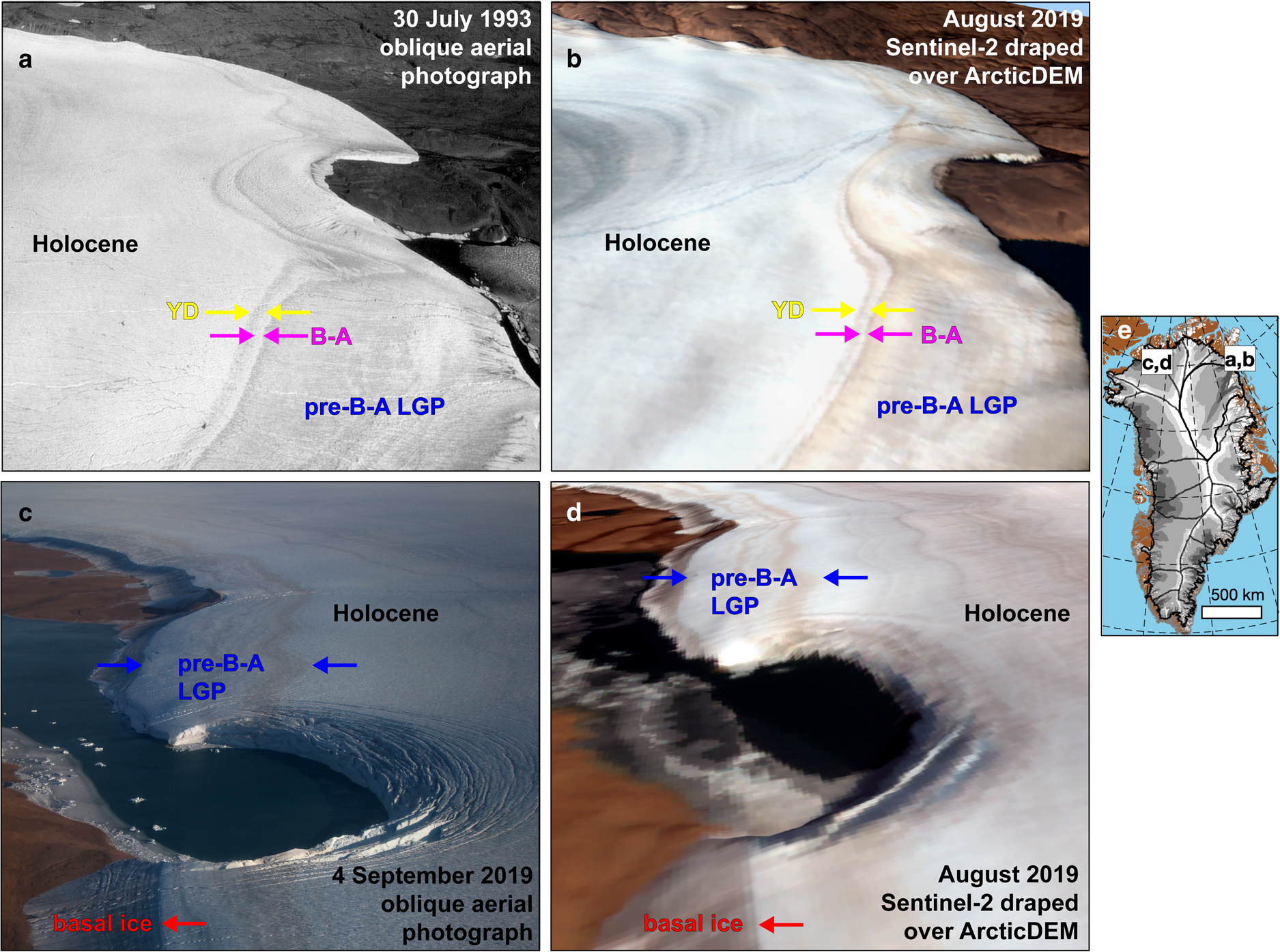
Fig. 2. (a) Oblique aerial photograph of GrIS margin taken 30 July 1993 from near the Kronprins Christian Land K site (Table 1) looking north–northeast (same as Fig. 2 of R02), with R02's original interpretation superimposed. Credit: H. Oerter. Reprinted from Annals of Glaciology with permission from the International Glaciology Society. (b) August 2019 S2 mosaic draped over 10-m ArcticDEM, with perspective and camera position oriented to approximately reproduce panel a and S2 colours contrast-stretched. No vertical exaggeration. (c) Oblique aerial photograph of GrIS margin adjacent to Daugaard-Jensen Land taken 4 September 2019 looking east–northeast, with age interpretation superimposed. Note that the YD and B-A layers are only faintly visible there and were not traced in the S2 mosaic. Credit: J. Sonntag. (d) Same as panel b, but for the site shown in panel c. (e) Map of Greenland showing the location of both sites, where greyscale is surface speed, as shown in Fig. 7. Contains Copernicus Sentinel-2 2019 data processed by ESA.
R02 did not directly georeference δ18O values to that oblique aerial photograph, so it was not immediately clear how well this relation holds there or elsewhere, but Bøggild and others (Reference Bøggild, Brandt, Brown and Warren2010) reported the patterns of surface dust concentration from this site that were consistent with R02's hypothesis. The success of later studies of ice-sheet surface geochemistry elsewhere across the GrIS further suggests R02's hypothesised relation is generally valid for coarsely identifying ice of the desired age (e.g. Petrenko and others, Reference Petrenko, Severinghaus, Brook, Reeh and Schaefer2006). Figure 2 shows unambiguously that the qualitative chronostratigraphic interpretation of R02 is reproducible using satellite imagery of Kronprins Christian Land and elsewhere in northern Greenland. Kjær and others (Reference Kjær2018) also reproduced the R02 photograph synthetically in a similar manner, from which they further argued that this interpretation is also qualitatively consistent with internal radiostratigraphy where it intersects the ice surface.
In general, the exact positions of R02's surface δ18O transects are not well known, likely because their collection predates the widespread use of global navigation satellite systems (GNSSs). Further, the azimuths of the surface transects were neither reported nor described, so we assume that they were roughly margin-perpendicular and prescribe these values with a precision of 5° (Table 1). R02 recognised this ambiguity, as not all authors were present during each sampling effort, and they described each site qualitatively with varying degrees of detail. Here we use a database that contains both δ18O values and along-transect distances for multiple R02 sites (H. Oerter, pers. comm., 2018). As needed, we translate the transect-origin locations manually with a precision of 10 m so that the most margin-proximal sample of each transect is at the ice-sheet margin (Table 1).
Table 1. Geographic data and applied translations for R02 δ18O surface transects

Sites are ordered following labelling given in Fig. 1, clockwise from the westernmost Warming Land site. Geographic coordinates are for the translated transect origin (typically near or at the ice margin). Note that the values for Warming Land sites are updated from R02 (N. Henriksen, pers. comm., 2018), and that site names are those given by R02. Translation azimuth is the direction in which the transect was translated horizontally, expressed clockwise from true north. The rightmost three columns are all estimated manually for this study.
In one case (Inglefield Land), the given position is nearly 9 km away from the present ice-sheet margin, an ambiguity noted by R02. We determined an approximate translation for this site to a location that is roughly consistent with a photograph of a portion of the margin visited by Risbo and Pedersen (Reference Risbo and Pedersen1994), who performed the sampling there. However, its location is too uncertain and the margin stratigraphy of this region is too complex to justify comparison of this δ18O transect with modern satellite imagery. Hence, we do not further consider this R02 site.
In late July 2019, we collected one additional surface transect near the southwest corner of Hiawatha Glacier, adjacent to Inglefield Land (Fig. 1), to better understand the chronostratigraphy of this complex margin. Ice samples were collected in a manner similar to that described by R02, i.e. several centimetres of surface crust were removed with an ice axe, then the ice was chipped from the underlying solid surface and placed into 60-mL polypropylene bottles. We collected 84 samples with a mean separation of 9.5 m and sampling locations were recorded with a GeodeTM mapping-grade GNSS receiver with sub-meter accuracy. The ice was then melted and both δ18O and δD (2H to 1H isotopic ratio) values of the resulting meltwater were measured by a mass spectrometer at the University of Oulu.
2.3. Layer tracing
To map potential chronostratigraphic units (layers) within the S2 mosaic based on contrasts in apparent surface brightness and colour, we examined the ice-sheet margin within the mosaic at a 1: 10 000 scale in QGIS version 3. We used local contrast stretching to improve visual boundary identification (typically min./max. stretch to 2–98% cumulative count), and traced boundaries manually. Where such boundaries were ambiguous, we did not trace them. We briefly explored alternative automated tracing schemes, including spectral band ratios, to identify individual layers. However, such schemes were typically challenged by variable cloudiness, solar elevation angle and the quality of preliminary versions of the mosaic, so we consider further development thereof beyond the scope of the present study. Our manual tracing approach is somewhat analogous to that of MacGregor and others (Reference MacGregor2015), who traced GrIS radiostratigraphy semi-automatically. We sacrifice deeper investigation of methodological sophistication and automation, which may enable rapid scalability in the future, so that at first, large-scale evaluation of northern GrIS margin surface stratigraphy can be generated.
Here we focus primarily on the boundaries that separate the four layers identified visually or described by R02. While additional visually distinctive layers are observed that appear to originate from both within and before the Holocene, these layers are not as widespread across the northern GrIS, nor were they identified visually by R02, nor were candidates ages assigned to them by that study.
We next describe these four boundaries in their typical stratigraphic order from top (highest exposed and farthest from the margin) to bottom (lowest exposed, at or closest to the margin). Figure 3 shows a simple ice-sheet cross-section illustrating these boundaries. The first boundary we traced is the bottom of the Holocene layer (i.e. its lowermost limit, 11.7 ka), which is identified by the characteristic sharp transition between white and light brown ice (Bøggild and others, Reference Bøggild, Brandt, Brown and Warren2010). The second is the bottom of the YD layer (12.8 ka), which directly underlies the Holocene layer, is typically a light brown colour and is relatively thin, i.e. the length of its margin-perpendicular horizontal exposure rarely exceeds ~200 m. This particular boundary is harder to trace because it is often less distinct than the others and it is closely sandwiched between the above Holocene boundary and the next meteoric boundary below it. The third boundary is the bottom of the B–A layer (14.7 ka), which is the bottom of the thin white layer that separates the dustier/browner YD layer above it from the darker brown pre-B-A LGP ice beneath it. Finally, we traced the upper boundary of what we assume is basal ice, which is significantly darker and greyer than the overlying Holocene or pre-Holocene ice and is typically not conformal to those meteoric strata. Hence, it has no specific age, although it typically underlies what appears to be pre-Holocene ice from within the LGP (115–11.7 ka). Tracing this boundary enables both better estimates of the horizontal length of surface-exposed pre-Holocene meteoric ice – rather than only using the ice margin – and also an opportunity to more broadly contextualise these basal ice exposures.

Fig. 3. Simplified cross-section of the margin of the northern GrIS illustrating the typical chronostratigraphy we mapped (circles). Boundary colours are the same as used for other figures. Not all boundaries were always detected, nor were they always found in this stratigraphic order due to occasional folding. Ice colour is exaggerated and approximates that which we observed following local contrast stretching when mapping boundaries at 1: 10 000 scale.
For WV imagery adjacent to Hiawatha Glacier and Warming Land, we retraced the four boundaries described above at finer scales (between 1:1000 and 1:2500), leveraging the finer resolution permitted by that imagery. For two locations adjacent to Warming Land, we also traced additional boundaries between alternating layers of whiter and browner ice in pre-B-A LGP ice that are not as distinct in the coarser-resolution S2 imagery.
To calculate plan-view distances between traced boundaries (the surface-exposed, horizontal layer thickness; not corrected for slope), we first determine the shortest distance between each digitised point and the ice margin or nunatak perimeter, whichever is closest. For each traced boundary, we then determine where each lower boundary (i.e. more margin-proximal) intersects the line that connects each of the upper boundaries' digitised points and the ice margin. In doing so, we approximate the margin-perpendicular horizontal exposure of each ‘layer’ (the stratigraphic unit between traced boundary pairs). All reported distances/thicknesses are great-circle arclengths on the surface of the WGS84 ellipsoid, not Cartesian distances within our default projection (EPSG:3413), which can differ by >2% at 80°N for the spatial scales we consider.
2.4 Ice-core data
To evaluate the apparent age of pre-B-A LGP ice, we use the NorthGRIP ice-core dust-concentration record produced by Ruth and others (Reference Ruth, Wagenbach, Steffensen and Bigler2003) using a laser microparticle detector. This record covers the time span between 60 and 9.5 ka, which is fortuitously contemporaneous with plausible chronostratigraphic interpretations of satellite imagery along part of the northern GrIS margin. While the interactions between dust, algae and seasonal subaerial melting are an area of active research (e.g. Ryan and others, Reference Ryan2018), for the purposes of this study we assume that the marginal surface stratigraphy whose boundaries we mapped can be compared qualitatively to this ice-core dust record from the dry snow zone (e.g. Bøggild and others, Reference Bøggild, Brandt, Brown and Warren2010).
3. Results
3.1. Satellite imagery at δ18O transects
Figures 4–6 show both the 2019 S2 mosaic and WV imagery in the vicinity of the available surface δ18O transects across the GrIS. These comparisons demonstrate that S2 and WV detect fundamentally the same margin stratigraphy. This consistency indicates that the coarser-resolution S2 imagery is sufficient to map key boundaries in surface stratigraphy across the GrIS.

Fig. 4. August 2019 S2 mosaic (left of pair) and WV imagery (right of pair) in the vicinity of available R02 δ18O surface-sampling sites in northern Greenland (Fig. 1), with δ18O data overlain at manually corrected position (‘adjusted site’), each transect's location uncertainty, and boundaries traced in S2 mosaic only shown for each pair. All image subscenes are contrast-stretched. For panels f and h, brighter snow remains along the margin that obscures the darker basal ice (evident in panels e and g), as was also observed in this region by Bøggild and others (Reference Bøggild, Brandt, Brown and Warren2010). WV sensor and image data are given in the title. Contains Copernicus Sentinel-2 2019 data processed by ESA. WV imagery is copyright 2020 DigitalGlobe Inc.

Fig. 5. August 2019 S2 mosaic (left of pair) and WV imagery (right of pair) in the vicinity of available R02 δ18O surface-sampling sites in southern Greenland (Fig. 1). The format follows Fig. 4. Contains Copernicus Sentinel-2 2019 data processed by ESA. WV imagery is copyright 2020 DigitalGlobe Inc.

Fig. 6. (a) August 2019 S2 mosaic and (b) 24 August 2018 WV image at the southwestern corner of Hiawatha Glacier, with δ18O values measured from surface ice samples collected in July 2019 overlain. Image sub-scenes are contrast-stretched. Boundary tracings shown are those mapped using each respective image, i.e. they were traced at substantially different spatial scales. (c) δ18O–δD co-isotope plot with values subdivided by margin region where they were detected. The reference global meteoric waterline is from Craig (Reference Craig1961). (d) Zoom-in of isotopic difference between meteoric and basal ice samples. Contains Copernicus Sentinel-2 2019 data processed by ESA. WV imagery is copyright 2020 DigitalGlobe Inc.
From these subscenes, it is clear that distinct margin surface strata are typically both more coherent and resolvable in northern Greenland, regardless of apparent age and potential sampling bias in the site selection of R02. While such strata have been identified reliably in southern Greenland previously from ground-based sampling and low-altitude aerial mapping (Petrenko and others, Reference Petrenko, Severinghaus, Brook, Reeh and Schaefer2006; Kurbatov and others, Reference Kurbatov2010), their surface expression in southern Greenland is ambiguous in the satellite imagery we examined, even in the finer resolution WV imagery. Only at the Pâkitsoq site, near where Petrenko and others (Reference Petrenko, Severinghaus, Brook, Reeh and Schaefer2006) sampled, is there a hint of coherent but heavily folded pre-Holocene strata in the WV imagery (Fig. 5j).
When compared against the estimated locations of the δ18O transects, we find that only the Kronprins Christian Land K/KS sites in northeastern Greenland display a plausible relation between δ18O and surface stratigraphy at the scale of these subscenes (Figs 4e–h), there, the transects are finely sampled (⩽5 m), the boundaries between the Holocene, YD and B-A layers are clear, and there is a clear transition in δ18O values between the LGP and the Holocene. The imprecision of available georeferencing and translation uncertainty prevents a finer-scale assessment of the relation between δ18O and the layering between the beginning of the B-A and the Holocene. At other sites in northern Greenland, either the coarseness of the δ18O sampling (Warming Land 1-4, Figs 4a–d), the length of the transect (Warming Land 1-4, Figs 4a–d), the imprecision of the georeferencing (Inglefield Land) or the lack of a clear transition in δ18O values, perhaps related to periodic surging (Storstrømmen N/NS, Figs 4i, j; Mouginot and others, Reference Mouginot, Bjørk, Millan, Scheuchl and Rignot2018) prevent additional confirmation of the large-scale chronostratigraphic relation hypothesised by R02. This situation limits us to Kronprins Christian Land K/KS as the type locality for the large-scale δ18O–stratigraphy relation that we seek to exploit (Fig. 2), but we note that this restriction does not impact the interpretation of the previously mentioned finer-scale investigations in southwestern Greenland (e.g. Pâkitsoq).
The new Hiawatha Glacier transect we collected is not as finely sampled as that of the R02 Kronprins Christian Land sites and its margin stratigraphy is more complex, with repeated sequences indicating folding (Fig. 6). However, its transitions in δ18O and δD values match well with satellite-mapped transitions in visual appearance, strongly supporting the δ18O–stratigraphy relation hypothesised by R02. The δ18O and δD values are not perfectly bimodal between glacial and interglacial periods, but that is expected given the significant variability that is typically present in those values. Further, the best-fit δ18O–δD relation differs significantly between meteoric ice (8.14 ± 0.07; 95% confidence bound) and what we assumed was basal ice prior to sampling (7.85 ± 0.18). Although this difference is small compared to global variability in that relation (e.g. Putman and others, Reference Putman, Fiorella, Bowen and Cai2019), it is consistent with previous observations of the isotopic differences between meteoric and basal ice (Larsen and others, Reference Larsen, Kronborg, Yde and Knudsen2010), further indicating that this layer is not meteoric.
3.2. Margin layer mapping
Our S2 mapping of the bottom of the Holocene, YD and B-A layers, along with the top of the basal ice, generated 242, 144, 145 and 241 discontinuous segments, respectively. These boundaries were mapped as far north as 82.1°N, adjacent to Peary Land in northern Greenland, and as far south as 74.2°N, adjacent to Waltershausen Glacier in eastern Greenland, but the boundary was mostly mapped north of 76.8°N. In terms of well-known major outlet glaciers in northern Greenland, we mostly mapped these boundaries from west of Hiawatha Glacier (northwest) to Storstrømmen (northeast). In terms of ice-drainage systems (Fig. 1), nearly all of the layer segments we mapped were within ice-drainage systems 1.1, 1.2, 1.3, 1.4 and 2.1, with a small portion mapped within system 2.2 (Zwally and others, Reference Zwally, Giovinetto, Beckley and Saba2012).
For the bottom of the Holocene layer, the median and maximum segment lengths are 4.2 and 89.5 km, respectively, with a median separation between digitised points of 91 m. The YD, B-A and basal ice boundaries were less extensively observed and mapped. Their median separation between digitised points was similar (79, 99 and 108 m, respectively), but their median segment lengths were somewhat shorter (1.7, 3.6 and 2.8 km, respectively) and their maximum segment lengths were substantially shorter (26.6, 44.3 and 39.4 km, respectively).
Figure 7 shows two combinations of the horizontal layer thickness between mapped boundaries. In the case of the pre-Holocene meteoric ice thickness, this metric represents an indirect proxy for the potential maximum age of coherent surface stratigraphy originating from periods of general interest. We note that this proxy is complicated by multiple factors, including the surface slope, subsurface boundary dip and the presence of any anomalous margin structures (e.g. plan-view folds). The combined thickness of the YD and B-A layers constitute a fixed period (1.1 + 1.9 = 3.0 kyr) that represents an indirect proxy for the age resolution within that period. While the resolution of the Landsat imagery used to generate the GIMP ice mask is 15 m and that of the S2 imagery is 10 m, we consider these thicknesses to have an uncertainty smaller than or comparable to that of the along-boundary digitisation separation (~100 m). This uncertainty is due to both the precision of our tracing and uncertainty in the delineation of the ice margin, which was traced in imagery nearly two decades older than that which we investigated (Section 2.1).

Fig. 7. (a) Horizontal thickness (distance) between the traced bottom of the Holocene layer and either the ice margin, nearby nunataks or the traced top of the basal ice layer, whichever is closest. Background greyscale on ice is surface speed (Joughin and others, Reference Joughin, Smith and Howat2017), and thick black lines are ice-drainage systems (Zwally and others, Reference Zwally, Giovinetto, Beckley and Saba2012). Layer-thickness symbols are scaled by both size and colour, with smaller values shown above larger ones. (b) Same as panel a but the horizontal thickness between the traced bottoms of the Holocene and B-A layers, i.e. the combined horizontal thickness of the YD and B-A layers. Note values assigned to thicknesses differ between panels a and b, per values on top and bottom of colour scale, respectively. Blue symbols denote R02 sites following Fig. 1. Abbreviations in panel a for regions/glaciers: IL: Inglefield Land; HiG: Hiawatha Glacier; HuG: Humboldt Glacier; DJL: Daugaard-Jensen Land; PG: Petermann Glacier; HL: Hall Land; NL: Nyboe Land; SG: Steensby Glacier; WaL: Warming Land; RG: Ryder Glacier; WuL: Wulffs Land; PL: Peary Land; JCCL: J.C. Christensen Land; MEL; Mylius-Erichsen Land; KFL: Kong Frederik VIII Land; KPL: Kronprins Christian Land; NG: Nioghalvfjerdsfjorden Glacier; LL: Lambert Land; ZI: Zachariæ Isstrøm; HOL: Hertugen af Orléans Land; ST: Storstrømmen; DLL: Dronning Louise Land.
The median horizontal thickness of pre-Holocene meteoric ice that we mapped is ~714 m (Fig. 7a, Fig. 8). This thickness is typically smaller in northwestern Greenland, as compared to northeastern Greenland. At lower latitudes in northeastern Greenland (<78°N), this thickness sometimes exceeds 2 km. However, these estimates are biased by more complex margin stratigraphy (folding) and the greater presence of nunataks there (e.g. Fig. 12, Appendix A; Section 3.3). Not all nunataks we observe in the S2 mosaic are present in the GIMP ice mask, leading to occasional spuriously high values we could not filter out easily. The thickest (in the margin-perpendicular sense) exposures of pre-Holocene ice occur along the GrIS margin adjacent to northeastern Inglefield Land, southern Daugaard-Jensen Land, southern Warming Land, southeastern Peary Land, southwestern Mylius-Erichsen Land, western Kong Frederik VIII Land, southwestern Kronprins Christian Land and the nunataks of Hertugen af Orléans Land south of Zachariæ Isstrøm (Figs 7a, 8). Elsewhere, such as southwestern Inglefield Land, such exposures can be near-contiguous for tens of kilometres, but their margin-perpendicular length is shorter and harder to interpret.

Fig. 8. Binned median horizontal thickness of each mapped layer (distance between either two traced boundaries or one traced boundary and ice margin), separated regionally by margin-adjacent land (vertical dashed lines) Abbreviations follow Fig. 7, and the number afterward is the GrIS drainage basin following Fig. 1. Along-margin bin length is 20 km. The horizontal scale bar panel is valid only within each land, i.e. it is not continuous between lands and there is an artificial 100-km buffer between each land's mapped exposures. Where the bottom (beginning) of the Holocene was mapped, but no other conformal boundaries below (older) than that, the layer is classified as ‘pre-Holocene’. (a) The western half of our study area, including the western half of Peary Land (‘PL (1/2)’). (b) The eastern half of our study area, beginning with the eastern half of Peary Land (‘PL (2/2)’). Note that these thickness distributions filter out nunatak-adjacent traced boundaries as best as possible, so Dronning Louise Land is not shown.
The median horizontal thicknesses of the YD and B-A layers were not significantly different (81 and 85 m, respectively), and their total median thickness (161 m; Fig. 7b) was less variable across the northern GrIS than the total thickness of pre-Holocene meteoric ice. We attribute this difference in spatial variability to two factors: (1) Their combined median thickness is only ~16 S2 pixels, so it was sometimes difficult to resolve at the fixed map scale we selected for mapping, and thinner exposures of these layers are likely undersampled. (2) This layer pair represents a fixed period of time (3 kyr), whereas the total thickness of pre-Holocene meteoric ice has no fixed period and may vary by tens of thousands of years. At the 10-m resolution of S2, the westernmost extent of detectable, coherent YD and B-A layers is northeastern Inglefield Land (Fig. 8), along the northeastern corner of Hiawatha Glacier; the easternmost extent is near Storstrømmen in Dronning Louise Land.
3.3. Anomalous margin layering
Having mapped the large-scale margin chronostratigraphy of the northern GrIS, we next briefly document anomalous and notable expressions of that stratigraphy (Fig. 9), in particular folded or unusually dark ice.
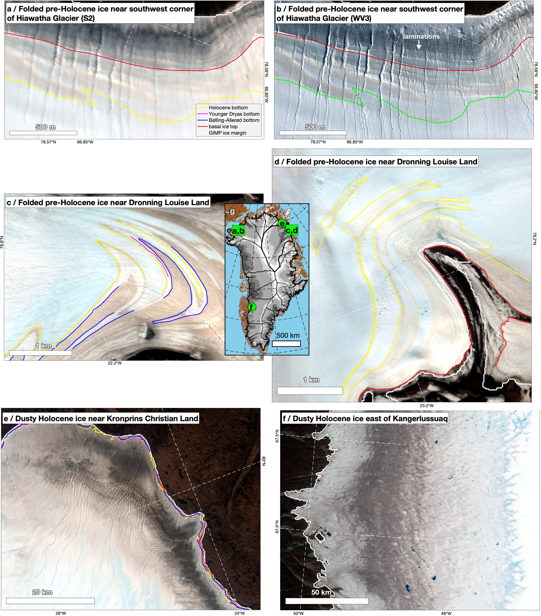
Fig. 9. Subscenes of contrast-stretched August 2019 S2 mosaic (except panel b, which is WV) showing example anomalous margin structures and layering across Greenland. (a) The ice-sheet margin southwest of Hiawatha Glacier in northwestern Greenland showing regular folding of pre-Holocene ice. (b) Same as panel a but using WV imagery. (c) and (d) Apparent plunging folds in emerging stratigraphy at the ice-sheet margin near Dronning Louise Land in northeastern Greenland. (e) The ice-sheet is bordering Kronprins Christian Land in northeastern Greenland and (f) east of Kangerlussuaq in southwestern Greenland, showing similar gray high-dustiness regions within Holocene ice. (g) Map of Greenland showing the location of subscenes, where grayscale is surface speed, as shown in Fig. 7. Contains Copernicus Sentinel-2 2019 data processed by ESA. WV imagery is copyright 2020 DigitalGlobe Inc.
With one major exception, the map trace of the pre-Holocene stratigraphy in the northwestern half of our study area (i.e. west of 45°W) generally conforms to either the ice margin or the mapped exposure of basal ice (Fig. 12). This exception is the ~35-km stretch of the ice margin immediately west of the southwestern corner of Hiawatha Glacier, Inglefield Land. There, the bottom of the Holocene undulates along-margin at kilometre scales with no discernible relation to the relatively uniform exposure of basal ice. Examination of both the S2 mosaic and finer-resolution WV imagery confirms this pattern and that the bottom of the Holocene ice appears to be repeated perpendicular to the ice margin at a scale of ~200 m (Figs 6, 9a, b). In map view, a portion of the pre-Holocene LGP sequence – but not all of it – is interfingered with Holocene ice. This pattern indicates that the Holocene–LGP boundary is steeply folded there relative to the surface slope, consistent with both the radar-sounding observations of Kjær and others (Reference Kjær2018) and the cross-sectional view put forth by Schaefer and others (Reference Schaefer2009) for a similar pattern within a smaller exposure in southwestern Greenland. The origin of this disturbance is unknown, but any plausible explanation must account for the remarkable horizontal extent of the folding and its apparent synchroneity.
East of ~32°W, plan-view lateral folding of identifiable boundaries occurs intermittently and mostly along the margins of outlet glaciers and nunataks (e.g. Figs 9c, d). This pattern suggests a plunging fold in the layering, i.e. one whose fold axis has a non-negligible dip relative to the near-horizontal ice surface. These folds could arise from past variability in the local ice-flow velocity field, as has been inferred for medial moraines at larger scales on Malaspina Glacier, Alaska (Post, Reference Post1972; Hudleston, Reference Hudleston2015). However, given that these folds are often seen near nunataks, which indicate locally non-negligible subglacial roughness, we consider it more likely that they are due to significant lateral shear as ice flows approximately these obstacles.
In the part of northeastern Greenland, north of Nioghalvfjerdsfjorden Glacier, we observe the extent of an unusually dark exposure of ice that clearly originated during the Holocene epoch and was previously identified by Bøggild and others (Reference Bøggild, Oerter and Tukiainen1996) (Fig. 9e). This dark ice is typically found within a layer that lies between ~2 and 5 km inland of the traced bottom of the Holocene and is adjacent to Kronprins Christian Land, where the type locality for the chronostratigraphic relation was first identified by R02 (Fig. 2). While we cannot yet assign a specific age range to this layer, its expression qualitatively resembles that of the better-known dark layer in southwestern Greenland (Fig. 9f), which also appears to be partly related to Holocene dust present in the ice (Bøggild and others, Reference Bøggild, Oerter and Tukiainen1996; Wientjes and others, Reference Wientjes2012; Ryan and others, Reference Ryan2018).
3.4. Potential oldest surface-exposed ice in Greenland
A question that naturally arises from our mapping is: where is the oldest ice? Our coarse mapping of chronostratigraphy of the northern GrIS margin reveals two distinct sites with extensive and coherent pre-Holocene stratigraphy that are ~38 km apart and adjacent to Warming Land (Fig. 10; Figs 13 and 14, Appendix A). Warming Land is the mostly deglaciated region bounded by Steensby Glacier to the west and Ryder Glacier to the east, both of which are major marine-terminating outlet glaciers in northern Greenland (Fig. 7a). At both sites, more than 20 >10-m-wide layers below the B-A are distinguishable and mostly conformable with each other. We distinguish these layers by their alternating pattern of colour and brightness, and they are typically detectable for several kilometres along-margin. For pre-B-A LGP layers at these two sites, there is no indication of plan-view folding, as observed elsewhere in northern Greenland (e.g. Figs 9c, d). This pattern suggests that layering at these sites is not repeated due to folding, but instead represents a contiguous period of ice deposition and subsequent flow.

Fig. 10. Contrast-stretched WV multispectral imagery of the GrIS margin adjacent to (a, c) southwestern and (b, d) southeastern Warming Land, in northern Greenland between Steensby and Ryder glaciers. Boxes between panels c and d identify potential matches in periods of higher apparent dust concentration between the two sites and (e) the dust concentration measured in the NorthGRIP ice core (Ruth and others, Reference Ruth, Wagenbach, Steffensen and Bigler2003). In panel e, the background color is scaled between blue (low dust concentration) and brown (high dust concentration) to illustrate potential matches. (f) Map of Greenland showing the location of relevant sites and estimated upstream origin of 55-ka ice, calculated using a Greenland-wide surface-velocity field (Joughin and others, Reference Joughin, Smith and Howat2017) and a shape factor of 0.8. WV imagery is copyright 2020 DigitalGlobe Inc.
Because we hypothesise that the layers' colour and brightness is primarily due to variable englacial dust concentration, following Bøggild and others (Reference Bøggild, Brandt, Brown and Warren2010), we compared the Warming Land sites' layering to the nearest available multi-millennial ice-core record of dust concentration, which is from the NorthGRIP ice core located more than 700 km southeast of these two sites (Figs 10e, f). We briefly explored the mathematical relation between NorthGRIP dust concentration and WV-observed colour but could not establish a simple relation, so this possibility is left to future investigations. Nevertheless, a qualitative but surprisingly good visual relation is apparent between the two sites' layering and the NorthGRIP dust record. Alternating browner and bluer layers exposed near Warming Land appear to be sequenced consistently with dustier and cleaner periods, respectively, in the NorthGRIP ice core. Further, the longer the dusty period in the NorthGRIP record, the wider the exposed dusty layer at Warming Land, with the same relation holding generally for less dusty periods and cleaner layers. We, therefore, hypothesise that the age of LGP ice exposed at these two sites extends back in time to a period well before to the Bølling–Allerød interval (i.e. older than 14.7 ka) – perhaps to before ~55 ka – and that multiple Dansgaard–Oeschger events are recorded there. While this apparent relation sets aside the potential complexity inherent to tens of millennia of ice flow between deposition in the ice-sheet interior and present-day emergence at the margin, this hypothesis can simply explain the remarkable correspondence between these independent records.
While R02 hypothesised the presence of surface-exposed ice from the Last Interglacial Period (Eemian; ~130–115 ka) elsewhere on the GrIS margin, that inference could not be confirmed by δ18O measurements alone. Hence, we suggest that the Warming Land sites discussed above represent the oldest coherent exposures of late-Pleistocene ice in the northern hemisphere identified so far. In Antarctica, yet older surface-exposed ice has been found in blue ice regions and the Dry Valleys (e.g. Schäfer and others, Reference Schäfer2000; Sinisalo and Moore, Reference Sinisalo and Moore2010; Buizert and others, Reference Buizert2014; Yan and others, Reference Yan2019).
3.5. Basal ice properties
During our satellite mapping of margin layering, we made four main observations of the basal ice layer that warrant reporting here. While we examined the northern GrIS margin at fine spatial scales, we also conducted a larger-scale examination of the whole of the GrIS margin. We found that the basal ice exposures detectable in the S2 mosaic were much more common in northern Greenland (our study area) than elsewhere. So, while we do not consider our mapping of the top of the basal ice to be comprehensive for the whole of Greenland, we consider it sufficient to support the following observations.
The first observation is that – when examined in finer-resolution WV imagery – the basal ice layer is itself laminated at multi-meter scales, as also reported by R02 but now visible at larger scales (e.g. Fig. 9b). This pattern is typically margin-parallel and suggests that the basal ice layer was formed episodically. It is not immediately clear if this pattern is consistent with the laminated basal ice facies that are sometimes observed in situ (e.g. Knight, Reference Knight1997). During our sampling at Hiawatha Glacier (Fig. 6), we also observed sub-meter laminations in the basal ice. Where supraglacial streams incised into the basal ice, these laminations were steeply dipping (subvertical).
The second observation is that – for any given traced segment of the top of the basal ice – this boundary appears to be approximately isochronal, as indicated by where/when it meets the Holocene or LGP ice above it (Fig. 12). This observation suggests that the apparent unconformity at this boundary is due to either an accumulation hiatus, ice erosion or basal freeze-on that occurred at approximately the same time. Further, the age at which this unconformity meets overlying younger ice appears to increase as one moves farther east and north across northern Greenland (Fig. 12). Adjacent to southwestern Inglefield Land, the top of the basal ice appears to intersect early Holocene ice, whereas adjacent to Warming Land or Kronprins Christian Land, that intersection appears to occur sometime during the pre-B-A LGP.
The third observation is that we mapped basal ice mostly adjacent to local highlands in the bed topography of northern Greenland (Fig. 11a). This observation is unsurprising, because we did not expect to be able to map surface-exposed layering extensively within or alongside most of the heavily sheared, major outlet glaciers that flow through subglacial troughs. However, it could be the most significant of the four, as it establishes a relatively simple spatial relation between the presence of surface-exposed basal ice and higher bed topography. The northern shear margin of Humboldt Glacier (southern Daugaard-Jensen Land) is perhaps the clearest deviation from that pattern, where basal ice is observed immediately adjacent to the subglacial trough that Humboldt Glacier flows through.

Fig. 11. The extent of basal ice layer superimposed on (a) BedMachine v3 bed topography (150-m grid; Morlighem and others, Reference Morlighem2017) and (b) the likely basal thermal state (5-km grid; MacGregor and others, Reference MacGregor2016b). Marker size for basal ice is scaled by its margin-perpendicular horizontal extent (thickness). For panel b, both mapped inland basal ice ‘plumes’ (Leysinger-Vieli and others, Reference Leysinger Vieli, Martin, Hindmarsh and Lüthi2018) and radiostratigraphy-inferred extent of the top of Eemian ice (115-ka isochrone) in the GrIS interior are overlain (MacGregor and others, Reference MacGregor2015); streamlines (solid lines) for basal units calculated using surface-velocity field (Joughin and others, Reference Joughin, Smith and Howat2017).
Finally, we note that basal ice is observed at the margin of ice-drainage systems that can be either predominantly frozen or thawed (Fig. 11b). Somewhat more basal ice appears present adjacent to predominantly frozen ice-drainage systems in far northern Greenland, but the margin abutting Daugaard-Jensen Land and Kronprins Christian Land is downstream of ice whose bed is likely thawed. Given the preservation of basal ice at these locations, this observation could reflect a limitation of the present basal thermal state synthesis (e.g. Chu and others, Reference Chu, Schroeder, Seroussi, Creyts and Bell2018). This observation also suggests that cold-based mechanisms likely contribute to the formation of the basal ice outcrops we mapped (Knight, Reference Knight1997). Very few of the basal ice ‘plumes’ identified by Leysinger Vieli and others (Reference Leysinger Vieli, Martin, Hindmarsh and Lüthi2018) – which they hypothesise are formed by basal freeze-on – are located beneath the ice that is presently flowing toward land-terminating margins (Fig. 11b). The radar-inferred distribution of Eemian ice is more widespread than the basal plumes (Fig. 11b), but it is difficult to constrain how thick such ice would be if any of it does indeed emerge at the margin.
4. Discussion
4.1. Implications for in situ margin sampling
A surprising outcome of our study is that – despite its successful subsequent application by later efforts – the visual pattern identified by R02 is only well supported by our comparison of satellite imagery and δ18O transects at a pair of adjacent sites in northeastern Greenland (Kronprins Christian Land K/KS, Figs 3, 4e–h) and our Hiawatha Glacier site (Fig. 6). We find that the sites sampled by R02 constitute a good diversity of expressions of margin layering, but for various reasons, the majority of them were suboptimal relative to their stated goal of producing ‘important and (cheap) supplements to ice core records’, particularly for the northern GrIS. This discovery does not invalidate in situ age interpretations at other sites, which often have more complex margin layering, because more detailed sampling commensurate to that layering complexity was performed, along with additional chemical analyses. However, this outcome does warrant additional surface sampling to refine the visual interpretation we applied across the northern GrIS.
Two previously unexplored sites of note are those that we identified along the ice margin adjacent to Warming Land, where surface-exposed strata are exceptionally well preserved and likely extend well into the LGP (Fig. 10). These identifications highlight the value of satellite remote sensing for site reconnaissance of ice-margin stratigraphy, because although these two promising sites are 38 km apart, they are both <6 km from opportunistic δ18O transects collected in 1985 (Table 1; Figs 4a–d). However, both sites are logistically challenging to reach, as they are more than 500 km from the nearest permanent settlement in Greenland and more than 200 km from Alert, Canada. This situation exemplifies the present balance of risk and reward for accessing surface-exposed paleoclimatically distinct ice in Greenland, i.e. the most promising sites are located in some of the most remote regions of the island.
The identification of additional promising sites for margin ice sampling in Greenland is also important for novel measurements of ice properties. While modern measurements of water isotopes and major ion concentrations require only a few millilitres of meltwater (e.g. Bailey and others, Reference Bailey, Klein and Welker2019), measurements of isotopic or mass concentrations of less common impurities in ice can either require or benefit from significantly larger samples (in some cases >100 kg) that far exceed those of typical ice cores or reasonable allocations thereof (e.g. Steig and others, Reference Steig, Morse, Waddington and Polissar1998; Petrenko and others, Reference Petrenko2009; Petaev and others, Reference Petaev, Huang, Jacobsen and Zindler2013; Buizert and others, Reference Buizert2014; Koll and others, Reference Koll2019). Wide surface exposures of apparently well-behaved layers in the northern GrIS offer the potential for effectively unlimited access to coherent Holocene and pre-Holocene ice at higher temporal resolution than has been possible for some methods that require bulk ice sampling. The northerly reach of these sites suggests they may also represent better proxies for past sea ice extent in the Arctic Ocean than existing deep Greenland ice cores, because surface-exposed ice there likely originates from farther north than those cores (Fig. 10f). However, recent work suggests that ice originating from the GrIS interior is unlikely to be as valuable as that from more coastal Arctic ice caps in constraining past sea ice extent (Rhodes and others, Reference Rhodes, Yang and Wolff2018).
4.2. Broader applications of mapping margin layering
The surface-exposed boundaries that we mapped constitute isochrones (or an unconformity, in the case of the top of the basal ice) that are direct visual analogues to those interfaces regularly mapped by radar sounding in the interior of the ice sheet. Shallow radar sounding of Antarctic blue ice areas has demonstrated correlations between mapped reflections and surface-isotopic profiles (e.g. Winter and others, Reference Winter2016). However, it is often difficult to trace deep radiostratigraphy within ~100 km of the GrIS margin with the most widely deployed radar sounders (MacGregor and others, Reference MacGregor2015; Florentine and others, Reference Florentine, Harper, Johnson and Meierbachtol2018), and we did not observe coherent surface stratigraphy in our S2 mosaic more than ~100 km inland of the margin because of persistent firn cover in the accumulation zone. Separately, we examined dozens of radargrams intersecting the northern margin that were collected in 2011 and 2014 by Operation IceBridge, and we found that they consistently failed to detect coherent radiostratigraphy there. Thus, the convergence of coherent surface- and radar-mapped layers is rare, but it has been demonstrated at Hiawatha Glacier by Kjær and others (Reference Kjær2018) using the latest radar-sounder technology.
Just as ice-sheet-wide maps of radiostratigraphy could be used to constrain and initialise ice-flow models (e.g. Clarke and others, Reference Clarke, Lhomme and Marshall2005; MacGregor and others, Reference MacGregor2016a; Born, Reference Born2017; Goelzer and others, Reference Goelzer2018), the surface layers mapped in this study could serve a similar purpose for models that can leverage this information. We are not aware of any large-scale model of the GrIS that is presently equipped to ingest these data directly, although Gilbert and others (Reference Gilbert2016) did find that a thermomechanical ice-flow model of the Barnes Ice Cap based on Elmer/Ice could successfully reproduce both the borehole-observed depth and the apparent rheological contrast of the Pleistocene–Holocene transition. We recognise that assimilation of these surface strata is unlikely to precede assimilation of radiostratigraphy for several reasons: (1) Observations of the former are not as widespread; (2) The horizontal separation of these boundaries is often significantly less than the spatial resolution of present-generation ice-sheet models; (3) Several additional processes complicate modelling of margin layering, as compared to radiostratigraphy in the accumulation zone (e.g. margin migration, surface melting, seasonally transient supraglacial and subglacial hydrology, formation and advection of basal ice).
While this study is the first to map pre-Holocene margin layering across a substantial portion of the GrIS margin, it has several limitations that could be improved upon in future efforts. Foremost is the clear improvement in boundary identification when using finer-resolution WV imagery. The five-to-eight-fold improvement in spatial resolution with only a single bit loss in radiometric resolution (as compared to S2) substantially improves the quality of our pre-Holocene boundary mapping (e.g. Fig. 10). However, the greater data volume of WV imagery and its reduced availability in northern Greenland during our period of interest (late summer) limited the utility thereof to specific narrow regions of interest (Figs 4, 9, 10). A second limitation is the use of manual boundary tracing, whose trade-offs were discussed in Section 2.2. A more substantial effort to investigate robust automated identification of surface-exposed layers could result in a more reliable and widespread mapping of GrIS margin stratigraphy, for both Holocene and pre-Holocene layers. Finally, we reiterate that additional in situ surface measurements of δ18O values and comparison with dated deep ice cores would improve confidence in the boundary ages that we have assumed in this study.
Our results also evince a potential terrestrial analogue to remote-sensing studies of ice masses elsewhere in the Solar System, in particular the northern polar layered deposits (NPLD) on Mars. There, numerous layers of variable dustiness are also observed by both satellite-based imaging and radar sounding (e.g. Christian and others, Reference Christian, Holt, Byrne and Fishbaugh2013; Lalich and others, Reference Lalich, Holt and Smith2019). These layers outcrop along the margins of the NPLD and have been linked statistically to nearby radiostratigraphy, but no in situ samplings has yet been performed, despite its potential value in deciphering recent Martian climate history. The northern GrIS is remote – but less so than Mars – and the warmer, faster GrIS is an imperfect analogue to the colder, near-static NPLD. However, future exploration of the margin of the northern GrIS could better constrain the geometric and englacial conditions that result in detectable surface and englacial stratigraphy. Such data could inform instrument requirements for future interplanetary missions to study the Martian climate history recorded by the NPLD (Smith and others, Reference Smith2020b).
4.3. The significance of northern Greenland's basal ice
An outstanding question raised by our examination of the northern margin of the GrIS is the significance of the widespread basal ice whose upper boundary we mapped (Fig. 11). Margin-exposed basal ice is famously complex, and our remote observations and limited in situ sampling cannot substitute for more detailed direct investigation thereof, so we cannot yet reliably interpret its apparent composition or formation mechanism from space (e.g. Knight, Reference Knight1997; Larsen and others, Reference Larsen, Kronborg, Yde and Knudsen2010). While our in situ measurements indicate that unit is indeed basal ice (Fig. 6), it is not yet certain that the unit we mapped can strictly be considered basal ice, as it is not consistently sediment-rich, nor have we demonstrated that all this ice has flowed within meters of the bed. Regardless, in the basal ice taxonomy put forth by Knight (Reference Knight1997), the most plausible interpretation is that we have mapped the top of dispersed facies, i.e. ‘ice that has been so affected by metamorphic processes close to the bed that it displays the features of neither meteoric glacier ice nor basally frozen ice.’ Such ice is expected to have a lower debris content than the dark brown ice-cemented debris layers sometimes observed at the base of Greenlandic glaciers (e.g. Larsen and others, Reference Larsen, Kronborg, Yde and Knudsen2010). This interpretation is consistent with the widespread geographic distribution of the unit (Fig. 11), but not with the occasional observations of distinct strata apparent in WV imagery (Figs 9a, b, 10; Figs 13, 14). However, Knight (Reference Knight1997) acknowledges that a continuum of basal ice facies is sometimes observed, and that stratified basal ice is more commonly observed below dispersed facies, which is roughly consistent with our observations and others in Greenland (e.g. Larsen and others, Reference Larsen, Kronborg, Yde and Knudsen2010).
Basal ice formation is generally attributed to cold-based glacier flow. While our basal ice distribution is somewhat consistent with being the downstream product of cold-based ice flow, it is not conclusively so, and the basal thermal state could easily have varied in the past (Fig. 11b). However, geologic observations of the deglaciated forelands across much of northern Greenland also suggest long periods of minimally erosive, cold-based glacier conditions, even during glacial periods with a greater ice extent (e.g. Pedersen and others, Reference Pedersen, Larsen and Egholm2019). A simple synthesis of those observations and ours could be that – outside of the tributary regions for major outlet glaciers and other anomalous subglacial structures – a frozen basal thermal state has persisted beneath the northern GrIS during most of the LGP and the Holocene. Otherwise, widespread pre-Holocene and basal ice are less likely to have survived and the deglaciated landscape would indicate greater long-term erosion rates. Absent additional direct observations of the ice unit whose top we mapped, the above arguments are speculative, but they can plausibly explain several of our observations and warrant further consideration – potentially as targets for studies of the past flow of the GrIS.
5. Conclusions
We synthesised existing observations of surface stratigraphy along the margin of the GrIS with a new satellite-based mapping of key boundaries in that stratigraphy along its northern margin. Effectively, we leveraged a decades-old insight from field observations into the first large-scale evaluation of the age of the northern margin of the GrIS. We described both typical and anomalous margin exposures across northern Greenland and identified promising sites for future recovery of paleoclimatically valuable ice, of which two sites adjacent to Warming Land hold the most promise. We find that large exposures of basal ice are more common across the margin of the northern GrIS than previously known, but that the significance of these exposures remains unclear. We speculate that they indicate the long-term persistence of cold-based conditions beneath most of the northern GrIS.
This study was enabled by access to large volumes of satellite imagery that could be processed efficiently and remotely into a mosaic of direct scientific value. Our approach favoured simplicity, speed and reliability in the mosaic generation and boundary tracing over methodological sophistication, and as a result, we were able to explore a large portion of the GrIS efficiently. We suggest that future remote-sensing studies of the GrIS and other ice masses considering similarly large scales use these resources to accelerate studies of difficult-to-access regions.
Supplementary material
The supplementary material for this paper can be found at https://doi.org/10.1017/jog.2020.62 The JavaScript code used to generate the filtered August 2019 S2 mosaic within Google Earth Engine is provided in Supplementary File 1 as a plain text file. The layer boundaries we traced are available as ESRI shapefiles in Supplementary File 2 as a zipped archive, for which the projection used is EPSG:3413 (NSIDC Sea Ice Polar Stereographic North). Supplementary Files 3–5 are video animations whose snapshots are shown in Figs 12–14, respectively (Appendix A), and have a standard 1080p resolution in MPEG-4 format. The frame rate of Supplementary File 3 is 2 fps for easy pausing between scenes and boundary overlays, whereas, for Supplementary Files 4, 5, it is 30 fps.
Data
Some of the satellite data presented in this paper are freely available and archived online. In particular, the S2 mosaic is presently available as a cloud-served basemap within the ITS_LIVE QGIS project file for Greenland (Gardner and others, Reference Gardner, Fahnestock and Scambos2020). The source URL for that mosaic can be added as a raster layer within any QGIS project. The MATLAB script used to process the data used in this study and to generate the figures is freely available from the corresponding author (JAM) upon request.
Acknowledgements
We thank the Goddard Fellows Innovation Challenge for supporting JAM's fieldwork and data analysis. We thank ESA/Copernicus for unrestricted access to the S2 imagery used in this study and Google Earth Engine for free access to their cloud computing resources. We thank the Polar Geospatial Center (PGC) and DigitalGlobe Inc. for access to WV imagery, and the PGC for ArcticDEM. We recognise the pioneering efforts of the late Niels Reeh, whose work provided both the inspiration and basis for this study. We thank Hans Oerter for providing a digital copy of δ18O data collected several decades ago and permission to use his photograph, and Niels ‘Oscar’ Henriksen for improved coordinates of the four Warming Land sites and valuable discussions concerning sampling methods there. We thank Pierre Beck, Anders Bjørk, Ludovic Brucker, Jessy Jenkins, Hans-Peter Marshall, Jérémie Mouginot and Lincoln Pitcher for equipment loans and fieldwork assistance, and John Sonntag for permission to use his photograph. Finally, we thank Chief Editor Hester Jiskoot, Scientific Editor Beatá Csathó and two anonymous reviewers for their constructive reviews of the manuscript.
Author contributions
All authors contributed to both the data interpretation and writing. JAM conceived the study and led the fieldwork, data analysis, interpretation and writing. MAF led the mosaic generation, WTC led the data archaeology, NKL and KKK led the interpretation of the basal ice mapping, and JMW led the laboratory analysis.
Appendix A
Animations
See Figures 12–14.

Fig. 12. Snapshot of Supplementary File 3. All traced boundary segments showed sequentially, clockwise about northern Greenland. A sub-scene of the S2 mosaic is generated for each digitised point with a 1-km buffer, then contrast-stretched to emphasise margin stratigraphy. Note that the scale for each frame varies depending on segment length, but that it is typically larger than that at which we traced boundaries in the imagery (1: 10 000). Contains Copernicus Sentinel-2 2019 data processed by ESA.

Fig. 13. Snapshot of Supplementary File 4. A rotation about a 3-D representation of Fig. 10a, i.e. the same WV subscene draped over ArcticDEM. Vertical exaggeration is 5x. WV imagery is copyright 2020 DigitalGlobe Inc.


 Open access