


Introduction
For some ice-mass configurations – confluences of tributaries, valley glaciers with high curvature of the centerline, ice sheets – the explicit treatment of transverse variations of the flow may yield better results than representing them in parameterized form in a one-dimensional model. The one-dimensional parameterization is effected by introducing shape factors, which have a partly theoretical, partly empirical basis. A two-dimensional flow model – by which is meant that there are two independent horizontal space coordinates (x, y) – avoids the need for shape factors to parameterize the transverse variations.
Whatever a model′s dimensionality, its application to an actual ice mass must begin by obtaining a set of initial conditions that are consistent with respect to the particular form of the dynamic equations employed by the model, including the continuity equation, and that are faithful, within the bounds of observation error, to the available field data. If they are not consistent, the model would rapidly redistribute the mass, not as a realistic projection of the future behavior of the ice mass but, artificially, to reconcile the inconsistencies. Slight errors in the velocity data can be amplified into spuriously large changes in glacier thickness.
If a particular form of the flow law is not assumed, the data must still be consistent with respect to the continuity equation. Such a data set, obeying continuity and faithful to the field data, would be useful in estimating the numerical values of the flow-law parameters and the amount of sliding motion.
Adjusting data to be consistent is much more difficult in two dimensions than it is in one. Velocity adjustment in one dimension is easy: flow enters an element at one side, it leaves at the other side, and the difference between the two fluxes equals the integral over the element of the difference between the mass balance and thickness change. Beginning with an assumed or estimated flux value at one end of a one-dimensional domain, a simple integration gives values directly at all the other nodes. In two dimensions, however, it is not always obvious whether any particular side of an element carries inflow or outflow. If the flow is roughly parallel to one axis of a two-dimensional grid, then clearly the up-stream side has inflow, and the down-stream side has outflow, but the lesser flow across the other two sides may have either sign. Or, if the flow is diagonal to a two-dimensional grid, so that the sign of the flux across each side is obvious, there is still not a one-to-one correspondence between the flux across one side and the flux across another side; this one-to-one correspondence is what makes the one-dimensional adjustment algorithm so simple, and so compact.
Also, a complete solution, in which all the variables are adjusted, is more difficult than a partial solution, in which only one is adjusted and the others are taken to be exact. The velocity and thickness appear non-linearly, as a product, in the continuity equation. Different adjustment criteria may be appropriate for different variables. The number of values to be adjusted is greater in a complete solution, which substantially increases the amount of computation.
Developed here is an algorithm that:
-
(a) adjusts only the velocity and assumes the other variables to be known, including the glacier thickness and the ratio of the surface velocity to the average velocity in the vertical column;
-
(b) requires values of all variables on a square grid, including initial estimates of the velocity; but requires no special conditions on the boundary;
-
(c) produces velocity values exactly satisfying a central-difference form of the continuity equation;
-
(d) uses a non-iterative procedure that minimizes the magnitude of the adjustment of the original velocity values, either the absolute adjustment or the relative adjustment; and
-
(e) is applicable to an arbitrarily shaped solution region.
Also developed is a compact, sub-optimum, well-behaved iterative procedure for transforming part of the velocity adjustment into a thickness adjustment.
Continuity Equation
The horizontal ξ-axis is taken to be positive in the direction of the flow, and the z-axis is taken to be vertical, positive upwards (Fig. 1). The horizontal component s of the glacier velocity at the surface Z is assumed to be the sum of a sliding part s B, which is constant with z, and a part S D due to deformation under simple shear that varies according to a power law in z:

in which A and n are the flow-law parameters, ρ is the ice density, g is the acceleration due to gravity, and the surface slope α is positive if the surface slopes down in the direction of flow. The bed slope is assumed not to differ markedly from the surface slope and it is also assumed that there are no gradients of longitudinal stress or basal or sidewall drag. The value at the surface z = Z is denoted s D and similarly for other variables, but below the surface (Z B ≤ z < Z) it is denoted s D(z). If sD (z) = 0 at the glacier bed z = Z B, then on performing the integration through the glacier thickness, h = Z – Z B,
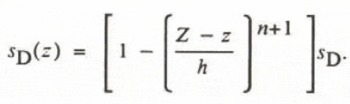

Fig. 1. Vertical section through the glacier thickness. The horizontal coordinate ξ is in the direction of the glacier flow.
The area flux q D (volume flux per unit width) from the deformational part is obtained by another vertical integration:

so that the total flux is
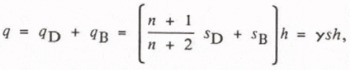
which, when the factor y is introduced, is expressed in terms of the thickness and the surface velocity. From Equation (4), since s = s D+ s B.
A characteristic thickness ![]() may be introduced; its product h
s with the surface velocity gives the same flux q as the integral of the actual velocity profile through the actual thickness.
may be introduced; its product h
s with the surface velocity gives the same flux q as the integral of the actual velocity profile through the actual thickness.
The foregoing is an idealized formulation, based on several simplifying physical assumptions, for determining y. A more precise and complete formulation would be appropriate only if sufficient data existed for applying it. What follows, however, as stated essentially by point (a) above, pertains to a data set in which y is specified, by whatever means may be used. Moreover, it is the product yh that is used in conjunction with the surface velocity, and in actual practice difficulties may arise in determining h accurately as well as in determining y.
When the surface velocity ![]() is referred to an arbitrary horizontal coordinate system, with components u in the x-direction and v in the y-direction, the speed is s = (u
2 + v
2)2. Considering an infinitesimal element in the x y plane, and assuming the density ρ to be constant, the conservation of mass may be expressed in the form of the continuity equation as
is referred to an arbitrary horizontal coordinate system, with components u in the x-direction and v in the y-direction, the speed is s = (u
2 + v
2)2. Considering an infinitesimal element in the x y plane, and assuming the density ρ to be constant, the conservation of mass may be expressed in the form of the continuity equation as

in which ![]() is the time rate of change of the thickness, assuming
is the time rate of change of the thickness, assuming ![]() is the net ice balance at both the top and the bottom of the column, as well as from exchange with englacial liquid-phase water. Equation (6) may be approximated by central differences on a square grid with spacing ∇x () as
is the net ice balance at both the top and the bottom of the column, as well as from exchange with englacial liquid-phase water. Equation (6) may be approximated by central differences on a square grid with spacing ∇x () as

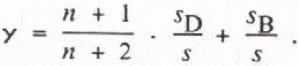
(fig.2) Horizontal coordinate system, grid indices, and solution region of a hypothetical problem. The symbols u, v, and ![]() indicate whether one, the other, or both components are to be adjusted.
indicate whether one, the other, or both components are to be adjusted.
Slight errors in the velocity data – one source of which is the interpolation of field data to the grid nodes — can produce large residuals in Equation (7). An error in one of the velocity components may be small relative to s, but it will generally be large relative to b – h; unless ∆x is very large compared with h, this will produce a large residual relative to F.
The Algorithm
The problem may be posed formally as finding the velocity field ![]() that satisfies continuity and that minimizes some measure of its difference from the original velocity field
that satisfies continuity and that minimizes some measure of its difference from the original velocity field ![]() . A least-squares form is used here for this measure, termed the adjustment magnitude,
. A least-squares form is used here for this measure, termed the adjustment magnitude,

which can be used to represent either the absolute adjustment, if λij = 1, or the relative adjustment, if. ![]()
If  and
and ![]() are any two fields satisfying Equation (6), then
are any two fields satisfying Equation (6), then
Therefore, given any field ![]() satisfying continuity, the problem is transformed into that of finding the field
satisfying continuity, the problem is transformed into that of finding the field ![]() that satisfies Equation (9) and that minimizes E. Because any vector that obeys a stream function is identically divergenceless, if the field
that satisfies Equation (9) and that minimizes E. Because any vector that obeys a stream function is identically divergenceless, if the field ![]() is defined by
is defined by

in which the scalar field ψ is the stream function, then Equation (9) is satisfied. If central-difference approximations

are used for the ψ-derivatives, then the central-difference approximations of Equation (9) is also exactly satisfied.
On substituting for (u 2) ij and (V 2) ij from Equations (11), and introducing them into Equation (8),

in which ![]() . Setting ∂E/∂Ψ
ij
to zero for all Ψ
ij
leads to the system of simultaneous linear equations:
. Setting ∂E/∂Ψ
ij
to zero for all Ψ
ij
leads to the system of simultaneous linear equations:

in which C
ij
= d
ij
/H
ij
and ![]() . Because the ψ-subscript increments are all ±2, the determination of ψij requires solving four separate systems of linear equations, one on each of the four independent, interlacing subsets (Table I, Fig. 3) of the grid nodes in the solution region. Each of the four linear systems is singly underdetermined – the ψ-differences are unaffected if a constant is added to all the ψ
ij
– which can be remedied by arbitrarily setting one of the to zero, say, and solving for the others. The matrix formed from the left-hand side of Equation (13) is sparse and diagonally dominant; each row contains the diagonal element and from two to four off-diagonal elements, depending on how many u or v values in the solution region surround ψ
ij
.
. Because the ψ-subscript increments are all ±2, the determination of ψij requires solving four separate systems of linear equations, one on each of the four independent, interlacing subsets (Table I, Fig. 3) of the grid nodes in the solution region. Each of the four linear systems is singly underdetermined – the ψ-differences are unaffected if a constant is added to all the ψ
ij
– which can be remedied by arbitrarily setting one of the to zero, say, and solving for the others. The matrix formed from the left-hand side of Equation (13) is sparse and diagonally dominant; each row contains the diagonal element and from two to four off-diagonal elements, depending on how many u or v values in the solution region surround ψ
ij
.
Table I Four Independent, Interlacing Subsets of the Solution Region. Indicated for each Subset are the Row and Column Combinations for Which the ψ -Values are Computed (from Equations 13), on which the u2, -values and V2,-values are then determined (from Equations 11), and on which the F-values are used to get the u1- values and v1-values (from Equations 14)


Fig. 3 Patterns of the four independent, interlacing subsets of the solution region, illustrating Table I. The key at the bottom shows to which subset each of the four corners of the pattern at each grid node pertains. For example, subset IV gives u-values on the even-row, odd-column nodes and it gives v-values on the odd-row. even-column nodes.
Because the ψ-field has the same number of degrees of freedom as the ![]() field which it produces, a globally optimum solution occurs. The number of degrees of freedom in the
field which it produces, a globally optimum solution occurs. The number of degrees of freedom in the ![]() field is the number of elements less the number of points at which Equation (7) is applied. The number of degrees of freedom in the ψ -field is one less than the number of its elements. Through Equations (11), the
field is the number of elements less the number of points at which Equation (7) is applied. The number of degrees of freedom in the ψ -field is one less than the number of its elements. Through Equations (11), the ![]() field is produced in terms of a
field is produced in terms of a ![]() field assumed to satisfy Equation (7). For instance, a parallel-flow solution for
field assumed to satisfy Equation (7). For instance, a parallel-flow solution for ![]() is
is

Although a mathematical proof cannot be adduced here, numerical experimentation revealed that the resulting ![]() field is independent of the
field is independent of the ![]() field used. Exactly the same
field used. Exactly the same ![]() field was obtained when
field was obtained when ![]() was obtained from Equations (14) by setting the u
ij
= 0 and making the v
ij
satisfy Equation (7), and also when another better resembling
was obtained from Equations (14) by setting the u
ij
= 0 and making the v
ij
satisfy Equation (7), and also when another better resembling ![]() was used with both u
ij
and v
ij
generally non-zero. The uniqueness of the solution
was used with both u
ij
and v
ij
generally non-zero. The uniqueness of the solution ![]() is confirmed intuitively by noting that E is a quadratic norm (Equation (8) and that the constraint is linear (Equation (7)).
is confirmed intuitively by noting that E is a quadratic norm (Equation (8) and that the constraint is linear (Equation (7)).
The topology of the solution region can be intricate. If the continuity equation is applied at some point (i, j), then F must be present there; u at (i, j+l) and (i, j–l); v at (i−1j) and (i+l+1); and ψ at (i−l, j+l), (i−l, j−l), (i+1j+1), and ((i+1, j−1)). Table 1 gives the patterns for each of the four independent, interlacing subsets of the solution region. Figure 2 shows a hypothetical solution region in terms of the nodes at which u and/or v are to be adjusted; it includes an unusual point (3,2) at which the continuity equation is applied, but at which only the u-component is to be adjusted. Figure 4 shows the corresponding subset II in terms of the patterns of F, u, v, and ψ.
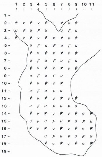
Fig. 4. Subset II of the solution region shown in Figure 2. The continuity equation is applied at nodes indicated by F to adjust components u and v at nodes indicated by those symbols by means of the stream function at nodes indicated by Ψ.
Adjusting Thickness Data
Consideration of Equation (7) reveals that if
h
and satisfy it at any point (i, j) then so do
h
p
and ![]() for any p > 0. This makes it easy to reduce the velocity adjustment E by transforming part of it into an adjustment of the
h
field. The magnitude of the compound adjustment, in which v is an arbitrary constant to scale, the contributions from the two variables,
for any p > 0. This makes it easy to reduce the velocity adjustment E by transforming part of it into an adjustment of the
h
field. The magnitude of the compound adjustment, in which v is an arbitrary constant to scale, the contributions from the two variables,

may represent either the relative or the absolute magnitude of the velocity adjustment, depending on how λ
ij
is assigned, and may represent either the absolute thickness adjustment, if μ
ij
= 1, or the relative adjustment if ![]() . Because the adjustment at one point is independent of the adjustments at other points, E′ can be minimized by minimizing the contributions from the individual points. However, this piecewise minimization, first E and then E′, does not produce as small an E′ as would occur were and
. Because the adjustment at one point is independent of the adjustments at other points, E′ can be minimized by minimizing the contributions from the individual points. However, this piecewise minimization, first E and then E′, does not produce as small an E′ as would occur were and ![]() adjusted simultaneously. The contribution at some point is minimized by setting
adjusted simultaneously. The contribution at some point is minimized by setting ![]() , which gives rise to the quartic polynomial (the subscripts having been dropped)
, which gives rise to the quartic polynomial (the subscripts having been dropped)
in which

The quartic may be rearranged into the convenient form

and may easily be solved iteratively. The function Φ(p) varies monotonically from Φ(0) = 1 and Φ(0)/dp = 0, to Φ(∞) = N/M and dΦ;(∞)/dp = 0. A good approximation is

which may suffice in some applications as itself an acceptable value of p or, if not, provides a first approximation for numerically solving Equation ( 17).


