


1. Introduction
Deep cavity oscillations are often found in many engineering applications, such as safety valves (Coffman & Bernstein Reference Coffman and Bernstein1980; Galbally et al. Reference Galbally, García, Hernando, de Dios Sánchez and Barral2015), closed side-branches in gas transport systems (Bruggeman et al. Reference Bruggeman, Hirschberg, van Dongen, Wijnands and Gorter1989; Ziada Reference Ziada2010) and turbomachineries (Ziada, Oengören & Vogel Reference Ziada, Oengören and Vogel2002; Aleksentsev, Sazhenkov & Sukhinin Reference Aleksentsev, Sazhenkov and Sukhinin2016), as well as in riverine environments (Perrot-Minot et al. Reference Perrot-Minot, Mignot, Perkins, Lopez and Riviere2020). Under certain flow conditions, the presence of airflow over a deep cavity can excite a self-sustained oscillation which couples with an acoustic mode to generate intense aerodynamic noises. Therefore, the necessity of minimising such acoustical problems arising from deep cavity oscillations deserves special attention.
The aerodynamic noise radiation by cavities owing to the presence of an incoming grazing flow has been studied by numerous researchers in the past. Early experimental evidence provided by Karamcheti (Reference Karamcheti1955), Heller, Holmes & Covert (Reference Heller, Holmes and Covert1971), Bilanin & Covert (Reference Bilanin and Covert1973), Tracy (Reference Tracy1997), Ashcroft & Zhang (Reference Ashcroft and Zhang2005), Thangamani, Knowles & Saddington (Reference Thangamani, Knowles and Saddington2014) and Wagner et al. (Reference Wagner, Beresh, Casper, DeMauro and Arunajatesan2017) have indicated that shallow cavities in a high-speed grazing flow emit intense acoustic radiation, which is composed of distinct and evenly spaced frequencies. The common cavity oscillation involves the self-sustained oscillation that ensues from the feedback mechanism of Rossiter (Reference Rossiter1964), where Kelvin–Helmholtz disturbances are amplified in the free shear layer and the impingement of disturbances on the downstream corner produces acoustic waves, which propagate upstream to excite further instabilities in the shear layer to close the feedback loop. However, for deeper cavities with larger aspect ratios (e.g.  $D/L \gg 1$), the feedback process involves the mutual interaction of the shear layer oscillation and a depthwise acoustic mode of the cavity (Elder Reference Elder1978; Ziada & Bühlmann Reference Ziada and Bühlmann1992), which generates aerodynamic noise of minimum damping (Tam Reference Tam1976; Koch Reference Koch2005). Consequently, the acoustic reinforcement near the upstream corner amplifies the flow instabilities into coherent vortices. The interaction of the latter with the downstream corner of the cavity translates into unsteady structural loadings and undesirable aerodynamic noises. Plumblee, Gibson & Lassiter (Reference Plumblee, Gibson and Lassiter1962) are among the first authors who investigated acoustic radiation by deep cavities. They observed that the maximum acoustic responses of deep cavities occurred at frequencies close to the depthwise acoustic modes, as was confirmed by East (Reference East1966) and Koch (Reference Koch2005). In general, cavity oscillations that involve the interplay between the shear layer oscillation and acoustic resonance are referred to as fluid-resonant oscillations according to Rockwell & Naudascher (Reference Rockwell and Naudascher1978). In this oscillation regime, the flow behaviour and the speculated mechanism that enables the self-sustained oscillation differ from the conventional Rossiter's feedback model. It is suggested that the resonant acoustic mode is the primary component that provides the upstream feedback, which strongly reinforces the shear layer oscillation (Tam & Block Reference Tam and Block1978; Tonon et al. Reference Tonon, Hirschberg, Golliard and Ziada2011; Ziada & Lafon Reference Ziada and Lafon2014).
According to Bruggeman (Reference Bruggeman1987), the acoustic response from a flow-induced oscillation in closed side-branches depends strongly on the ratio of the acoustic particle velocity associated with the depthwise standing-wave to the mean flow velocity and can be separated into three main categories: low; moderate; and high acoustic pulsation, with each level describing an increase in the influence of the acoustic resonance on the receptivity of the separated shear layer near the upstream corner. The level of pulsation is expressed by the ratio of  $|u_{a}|/U_b$, where $|u_a|$ is the amplitude of the acoustic particle velocity at the cavity opening and $U_b$ is the centreline velocity in the main channel. At low pulsation levels (e.g. $|u_{a}|/U_{b} \leqslant O(10^{-3})$), the acoustic perturbation is insufficient to trigger the formation of coherent vortices from the separated shear layer near the upstream corner. Consequently, the streamwise growth of the hydrodynamic perturbation in the shear layer is described by the linearised theory of an inviscid quasi-parallel free shear layer (Michalke Reference Michalke1972). At higher pulsation levels (e.g. $|u_{a}|/U_{b} \geqslant O(10^{-3})$), the shear layer roll-up into discrete vortices and the amplitude of oscillations is determined by the nonlinearities (Peters Reference Peters1993). Accordingly, Bruggeman et al. (Reference Bruggeman, Hirschberg, van Dongen, Wijnands and Gorter1989) suggested an alternative feedback mechanism for the fluid-resonant oscillation based on Vortex Sound Theory (Howe Reference Howe2003). This mechanism can be expressed by the following process: acoustic forcing from the resonance on the shear layer at the upstream corner; formation of coherent vortices by the instabilities in the separated shear layer; transfer of energy from the local flow to the acoustic field by the interaction of convective vorticity and the acoustic resonance; and the net energy transfer to the acoustic field determines the amplitude and the phase of the feedback at the upstream corner. Based on this concept, the acoustic resonance in the deep cavity plays an important role in destabilising the shear layer and reinforcing the vortex coalescences. Therefore, this alternative feedback mechanism based on the energy transfer between the vortical (hydrodynamic) and potential (acoustic) fields offers an attractive explanation for the ‘lock-on’ effect as observed in deep cavity experiments (East Reference East1966; Yang et al. Reference Yang, Rockwell, Cody and Pollack2009).
The present paper aims to provide an extended understanding of the feedback mechanism that reinforces the self-sustained oscillation in a deep cavity, with a particular interest in the modulation process of the shear layer oscillation and the vortex dynamics in the presence of acoustic resonance. Therefore, a central hypothesis of the present paper is that the Rossiter modes provide the primary sound source, which can be further amplified by the spatially coherent acoustic field from the acoustic resonance (Tam & Block Reference Tam and Block1978; Gutmark & Ho Reference Gutmark and Ho1983). Accordingly, a high-fidelity numerical simulation is performed, from which the time history of the hydrodynamic and acoustic fields are accurately captured around the deep cavity to facilitate the investigations.
This paper is structured and written in the following order. Section 2 introduces the computational set-up and methods used in this study. In § 3, the acoustic and hydrodynamic fields around the cavity region are investigated in detail. Section 4 moves the focus to the proposition of a modified Rossiter formula to consider the fluid–acoustic coupling mechanism of the deep cavity in acoustic resonance. Finally, concluding remarks are provided in § 5.
2. Description of problem and the computational set-up
A cavity section with a length of  $L/h=0.608$ and depth of $D/h=1.6$ enclosed in a channel with a height of $2h$ is considered in the present study. The Reynolds number based on the cavity opening length of $L = 0.038\ \textrm {m}$ is set to $Re_\infty =174\,594$, and a free stream Mach number of $M_\infty =0.2$ based on the ambient speed of sound (for air) of $a_\infty =340.2\ \textrm {m}\ \textrm {s}^{-1}$ and the reference temperature of $T_\infty =288$ K are considered in this work. The current numerical investigation employs a high-resolution implicit large-eddy simulation (ILES) method based on a wavenumber-optimised discrete filter (Kim Reference Kim2010). The filter is applied directly to the solution (conservative variables) at every time step. It acts as an implicit sub-grid scale (SGS) model that enforces dissipation of scales smaller than the filter cut-off wavelength. Garmann, Visbal & Orkwis (Reference Garmann, Visbal and Orkwis2012) performed an extensive analysis of the ILES technique, compared with the traditional implementation of an explicit SGS model, and concluded that ILES simulations are capable of correctly capturing the flow physics when the grid is subjected to an appropriate resolution.
2.1. Governing equations and numerical methods
In this work, the full 3-D compressible Navier–Stokes equations (with a source term for sponge layers included) are used, which can be expressed in a conservative form, transformed onto a generalised coordinate system as
 \begin{equation} \frac{\partial}{\partial t}\left(\frac{\boldsymbol{Q}}{J}\right)+\frac{\partial}{\partial\xi_i}\left(\frac{\boldsymbol{E}_j-Re^{{-}1}_\infty M_\infty\boldsymbol{F}_j}{J}\frac{\partial\xi_i}{\partial x_j}\right)={-}\frac{a_\infty}{L}\frac{\boldsymbol{S}}{J}, \end{equation}
where the indices  $i=1,2,3$ and $j=1,2,3$ denote the three dimensions. The vectors of the conservative variables, and inviscid and viscous fluxes are given by
 \begin{equation} \left. \begin{gathered} \boldsymbol{Q}=[\rho,\rho u,\rho v,\rho w,\rho e_{t}]^\textrm{T},\\ \boldsymbol{E}_j=[\rho u_j,(\rho uu_j+\delta_{1j}p),(\rho vu_j+\delta_{2j}p), (\rho wu_j+\delta_{3j}p),(\rho e_{t}+p)u_j]^\textrm{T},\\ \boldsymbol{F}_j=[0, \tau_{1j}, \tau_{2j}, \tau_{3j}, u_i\tau_{ji}+q_j]^\textrm{T}, \end{gathered}\right\} \end{equation}
with the stress tensor and heat flux vector written as
 \begin{equation} \tau_{ij}=\mu\left(\frac{\partial u_i}{\partial x_j}+\frac{\partial u_j}{\partial x_i}-\frac{2}{3}\delta_{ij}\frac{\partial u_i}{\partial x_i}\right), \quad q_j=\frac{\mu}{(\gamma-1)Pr}\frac{\partial T}{\partial x_j}, \end{equation}
where  $\xi _i=\{\xi ,\eta ,\zeta \}$ are the generalised coordinates, $x_j=\{x,y,z\}$ are the Cartesian coordinates, $\delta _{ij}$ is the Kronecker delta, $u_j=\{u,v,w\}$, $e_{t}=p/[(\gamma -1)\rho ]+u_ju_j/2$ and $\gamma =1.4$ for air. The local dynamic viscosity $\mu$ is calculated by using Sutherland's law (White Reference White1991). In the current set-up, $\xi$, $\eta$ and $\zeta$ are aligned in the streamwise, vertical and spanwise directions, respectively. The Jacobian determinant of the coordinate transformation (from Cartesian to the generalised) is given by $J^{-1}=|\partial (x,y,z)/\partial (\xi ,\eta ,\zeta )|$ (Kim & Morris Reference Kim and Morris2002). The extra source term $\boldsymbol {S}$ on the right-hand side of (2.1) is non-zero within the sponge layer only, which is described in Kim, Lau & Sandham (Reference Kim, Lau and Sandham2010a,Reference Kim, Lau and Sandhamb). In this paper, the free stream Mach and Reynolds numbers are defined as $M_\infty =U_\infty /a_\infty$ and $Re_\infty =\rho _\infty U_\infty L/\mu _\infty$, where $a_\infty =\sqrt {\gamma p_\infty /\rho _\infty }$ is the ambient speed of sound and $U_\infty =\sqrt {u^2_\infty +v^2_\infty +w^2_\infty }$ is the speed of the free stream mean flow. The governing equations are non-dimensionalised based on the streamwise cavity opening length $L=38$ mm for length scales, the ambient speed of sound $a_\infty$ for velocities, $L/a_\infty$ for time scales and $\rho _\infty a^2_\infty$ for pressure, unless otherwise notified. Temperature, density and dynamic viscosity are normalised by their respective ambient values $T_\infty$, $\rho _\infty$ and $\mu _\infty$.
The governing equations given above are solved using high-order accurate numerical methods specifically developed for aeroacoustic simulation on structured grids. The flux derivatives in space are calculated based on fourth-order pentadiagonal compact finite-difference schemes with seven-point stencils Kim (Reference Kim2007). Explicit time advancing of the numerical solution is carried out using the classical fourth-order Runge–Kutta scheme with the Courant–Friedrichs–Lewy number of 0.95. Numerical stability is maintained by implementing sixth-order pentadiagonal compact filters for which the cutoff wavenumber (normalised by the grid spacing) is set to  $0.85{\rm \pi}$. In addition to the sponge layers used, characteristics-based non-reflecting boundary conditions based on Kim & Lee (Reference Kim and Lee2000) are applied at the inflow and outflow boundaries to prevent any outgoing waves from returning to the computational domain. Periodic conditions are used across the spanwise boundary planes unless otherwise stated. Slip (no penetration) and no-slip wall boundary conditions based on Kim & Lee (Reference Kim and Lee2004) are applied at the top and bottom channel walls, respectively.
The computation is parallelised through the domain decomposition and message passing interface (MPI) approaches. The compact finite-difference schemes and filters used are implicit in space owing to the inversion of pentadiagonal matrices involved, which requires a precise and efficient technique for the parallelisation to avoid numerical artefacts that may appear at the subdomain boundaries. A recent parallelisation approach based on quasi-disjoint matrix systems (Kim Reference Kim2013) offering super-linear scalability is used in the present paper.
2.2. Simulation set-up and discretisation of the problem
The cavity geometry and the computational domain used in this work are shown in figure 1. The domain of investigation is composed of  $x/L\in [-1.64,4.93]$ in the streamwise direction, $y/L\in [-2.63,3.29]$ in the vertical direction and $z/L\in [0,0.822]$ in the spanwise direction. The entire computational domain, the inner region (physical domain) where meaningful simulation data are obtained, and the sponge layer zone are defined as
 \begin{align} \left. \begin{gathered} \mathcal{D}_\infty=\{\boldsymbol{x}\,|\,x/L\in[{-}1.644,4.934],y/L\in[{-}2.632,3.289],z/L\in[0,0.822]\},\\ \mathcal{D}_{physical}=\{\boldsymbol{x}\,|\,x/L\in[{-}1.644,3.289],y/L\in[{-}2.632,3.289],z/L\in[0,0.822]\},\\ \mathcal{D}_{sponge}=\mathcal{D}_\infty-\mathcal{D}_{physical}. \end{gathered}\right\} \end{align}
The physical domain  $\mathcal {D}_\infty$ consists of a deep cavity with an aspect ratio of $D/L=2.632$ enclosed in a straight rectangular channel with a channel half-height of $h/L=1.644$. The channel region is discretised by a total of $720\times 270\times 180$ grid points in the streamwise, vertical and spanwise directions, respectively. A total of $180\times 180\times 180$ grid points are used in the streamwise, vertical and spanwise directions, respectively, in the cavity region. The mesh in the wall-normal direction is refined close to the viscous wall $y^{+}\approx 1$ to ensure a sufficiently high level of near-wall grid resolution is maintained throughout the viscous wall surfaces.

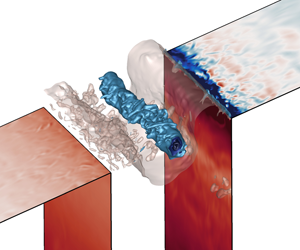
Figure 1. Visualisations of the current computational domain of the deep cavity configuration enclosed in a channel. (a) Instantaneous non-dimensional  $Q$-criterion iso-surfaces ( $Q=0.15$) coloured by the non-dimensional vorticity magnitude ( $|\omega _{i}|$), showing the three-dimensional vortices in the turbulent boundary layer. (b) A spanwise view of the computational domain used in the current numerical investigation.
The inlet is located at  $x/L=-1.664$ upstream of the cavity where the turbulent inflow data is injected. The outflow boundary is placed at a relatively remote location downstream from the cavity, which allows a sufficient distance for the vortices to dissipate. In the current study, a precursor simulation is employed to generate the prerequisite turbulent inflow data for the cavity simulation. The precursor simulation domain size ( $L_x\times L_y\times L_z$) was set to $4\delta _{99}\times 1\delta _{99}\times 2\delta _{99}$ with $360\times 120\times 180$ grid points in the streamwise, vertical and spanwise directions, respectively. The initial boundary layer thickness $\delta _{99}$ was determined analytically based on Na & Lu (Reference Na and Lu1973), and the channel flow was initialised with the turbulent mean flow profile according to Spalding (Reference Spalding1961). Periodic boundary conditions were applied in the streamwise and spanwise directions and an implicit pressure gradient to maintain the desired mass flow rate was applied. The precursor simulation was completed when the mean flow profile was converged and the obtained instantaneous flow solutions were injected into the cavity simulation through the inlet plane. Figure 2 shows a close agreement of the time-averaged turbulent velocity profile and the Reynolds stresses between the current half-channel LES and the full-channel DNS results from Lee & Moser (Reference Lee and Moser2015), conducted at $Re_{\tau }\approx$ 2600 and 2000, respectively. The frequency spectra of the incoming turbulence are shown in figure 3 and the inflow boundary layer information for the current simulation is listed in table 1.

Figure 2. (a) Time-averaged turbulent boundary layer profile and (b–d) Reynolds stresses obtained from the current precursor half-channel LES ( $Re_{\tau }\approx 2600$) compared with the full-channel DNS ( $Re_{\tau }\approx 2000$) by Lee & Moser (Reference Lee and Moser2015).

Figure 3. The power spectral density (PSD) of the streamwise velocity fluctuation  $u'$ (solid line); vertical velocity fluctuation $v'$ (dashed line); and spanwise velocity fluctuation $w'$ (dash–dotted line) of the precursor simulation measured on the outlet plane in the log-law region (e.g. $y^{+}=500$), superimposed with the tonal frequencies (dotted line) observed from figure 5(b).
Table 1. Boundary layer parameters used as the inflow condition of the current cavity simulation.
2.3. Definition of variables for statistical analysis
Data processing and analysis were carried out upon the completion of the simulation. The main property required in this study was the PSD function of the pressure fluctuation around the cavity. To facilitate the following discussions, the pressure fluctuation is defined here as
 \begin{equation} p'(\boldsymbol{x},t)=p(\boldsymbol{x},t)-\bar{p}(\boldsymbol{x}), \end{equation}
where  $\bar {p}(\boldsymbol {x})$ is the time-averaged pressure field. Following the definitions used in Goldstein (Reference Goldstein1976), the PSD functions of the pressure fluctuations (based on frequency and being one-sided) are then calculated by
 \begin{equation} S_{pp}(\boldsymbol{x},f)=\lim_{T\rightarrow\infty} \frac{P(\boldsymbol{x},f,T)P^*(\boldsymbol{x},f,T)}{T}, \end{equation}
where  $P$ is an approximate Fourier transform of $p$, respectively, based on the following definition of
 \begin{equation} P(\boldsymbol{x},f,T)=\int_{{-}T}^{T}{p'(\boldsymbol{x},t)\ \textrm{e}^{{-}2{\rm \pi} ift}\, \text{d} t}, \end{equation}
and ‘ $*$’ denotes a complex conjugate. Similarly, the magnitude and the respective phase of the single-sided Fourier transform pressure field are calculated by
 \begin{gather} \left|P(\boldsymbol{x},f,T)\right|=2 \sqrt{P(\boldsymbol{x},f,T)P^{*}(\boldsymbol{x},f,T)}, \end{gather}
 \begin{gather}\varPhi_{p}(\boldsymbol{x},f,T)=\arctan \left\{ \frac{ \text{Im}[P(\boldsymbol{x},f,T)] }{\text{Re}[ P(\boldsymbol{x},f,T)]} \right\}. \end{gather}
In the above equations,  $T$ represents the half-length of the time signals used for the approximate Fourier transform. The same procedures are also performed on the velocity field later in this paper.
3. Results and discussion
The self-sustained oscillation in deep cavities is often described as a fluid-resonant oscillation, in which the shear layer oscillation couples with a depthwise acoustic mode of the cavity. When this happens, a distinct large-scale vortical structure will be reinforced by the acoustic resonance, and its interaction with the downstream corner promotes a maximum conversion of local flow energy into acoustic energy. This process is captured in the current computational results. The iso-contour of the pressure fluctuation illustrated in figure 4(a) shows a low-pressure region caused by the concentrated vorticity (not shown) near the cavity opening, and the wall-pressure contours indicate the predominance of compressive acoustic waves inside the cavity before the vortex impingement. Furthermore, a noticeable low-pressure region near the top surface of the downstream wall that ensues from the separated flow is observed and will be scrutinised later in § 3.2. Subsequently, figure 4(b) shows the instant when the vortical structure induces a sufficient downwash velocity to reattach the flow downstream. The reattachment of the flow causes the separation region to disappear. A rapid alteration of the pressure fluctuation in the cavity follows afterwards to signify subsequent rarefaction wave emissions.

Figure 4. A large-scale vortical structure identified using the iso-contour of an instantaneous pressure fluctuation. Note that the flow is from left to right. The convection of the large-scale vortical structure and the associated change in wall-pressure fluctuation, (a) prior to the impingement and (b) after the impingement on the downstream corner, illustrate the aerodynamic noise emissions.
3.1. Pressure fluctuations and oscillation frequencies
In this section, the focus is placed on the acoustic waves that manifest as the pressure fluctuates in the cavity. To realise this, the simulation is performed for 608 000 time steps to attain a non-dimensional time of 100 for the wall-pressure at the cavity base to reach a steady-periodic state. Figure 5(a) shows the time signals of the wall-pressure fluctuation measured on the cavity base at three different streamwise positions, which converge to a similar solution after approximately  $ta_{\infty }/L=100$. Subsequently, Fourier transform is carried out on an additional non-dimensional time of approximately 540 samples (every 0.325 time unit) of the computational data over a total duration of non-dimensional time of 175, which corresponds to approximately 13 periods of the fundamental frequency. The resulting time signals are approximately periodic in time and any steady component is removed prior to the Fourier transform. Different windowing functions were attempted and the results show the comparable spectrum composition. Figure 5(b) shows the respective PSD of the wall-pressure signals where a fundamental frequency peak was observed at $fL/a_{\infty } =0.077$ and the rest were superseded by higher harmonics. The invariance of the spanwise-averaged wall-pressure fluctuation with respect to different streamwise locations on the cavity base can be understood by the fact that the wavelength of the acoustic field is much longer than the streamwise characteristic length of the cavity (i.e. $\lambda _{a} \gg L$). Therefore, the cavity is assumed to be acoustically compact and the acoustic waves in the cavity can be modelled by a one-dimensional depthwise standing wave. This is a reasonable approximation in deep cavity configurations as the depth is usually longer than that in the streamwise direction. The pressure fluctuations around the cavity can be characterised into two main regions, which are a local hydrodynamic fluctuation near the cavity opening and an acoustic fluctuation around the cavity. Therefore, it is essential to decompose these pressure fields into the hydrodynamic and acoustic components to facilitate the investigations. To achieve this, we employed the momentum potential theory (MPT) developed by Doak (Reference Doak1989). Specifically, in Doak's MPT, the momentum density $\rho \boldsymbol {u}$ is separated into rotational and irrotational components through a Helmholtz decomposition. The Helmholtz decomposition of $\rho \boldsymbol {u}$ may be written as
 \begin{equation} \rho\boldsymbol{u}=\boldsymbol{B}-\boldsymbol{\nabla}\psi, \quad \boldsymbol{\nabla} \boldsymbol{\cdot} \boldsymbol{B} = 0, \end{equation}
where  $\boldsymbol {B}$ and $\boldsymbol {\nabla }\psi$ are the solenoidal and irrotational components of $\rho \boldsymbol {u}$, respectively. Substituting (3.1a,b) into the continuity equation yields a Poisson equation for the irrotational component, with a source term dependent on density fluctuations,
 \begin{equation} \nabla ^2 \psi = \frac{\partial \rho}{\partial t}. \end{equation}
For a single phase continuum fluid,  $\psi$ is separated into an acoustic component (irrotational and isentropic, denoted $\psi _{A}$) and an entropic component (irrotational and isobaric, $\psi _{E}$), which are governed by the exact equations
 \begin{equation} \psi=\psi_{A}+\psi_{E}, \quad \nabla^2 \psi_{A}=\frac{1}{c^2}\frac{\partial \rho}{\partial t}, \quad \nabla^2\psi_{E}=\frac{\partial \rho}{\partial E}\frac{\partial E}{\partial t}. \end{equation}
Considering the low Mach number in this study, the entropy (thermal) contribution is assumed to be relatively small compared with the acoustic contribution, and therefore  $\psi _E$ is not included in the subsequent calculation. Then, the momentum equation in terms of the hydrodynamic and acoustic components is obtained by substituting (3.1a,b) into the momentum equation, expressed as
 \begin{equation} \frac{\partial}{\partial t}(\boldsymbol{B}-\boldsymbol{\nabla}\psi) + \boldsymbol{\nabla} \boldsymbol{\cdot} \left[\frac{(\boldsymbol{B}-\boldsymbol{\nabla}\psi)(\boldsymbol{B}-\boldsymbol{\nabla}\psi)}{\rho}-\tau_{ij}\right] + \boldsymbol{\nabla} p =0. \end{equation}
By taking the divergence of (3.4), the Poisson equation for the hydrodynamic pressure fluctuation  $p'_{H}$
 \begin{equation} \nabla^2 p'_{H} = S_{H} +\widetilde{S_{H}}, \end{equation}
and the Poisson equation for the acoustic pressure fluctuation  $p'_{A}$
 \begin{equation} \nabla^2 p'_{A} = S_{A} +\widetilde{S_{A}}, \end{equation}
are derived. Accordingly, the hydrodynamic and acoustic pressure fluctuations are obtained by solving the Poisson equations in (3.5) and (3.6), respectively. The numerical implementation is described extensively in Unnikrishnan & Gaitonde (Reference Unnikrishnan and Gaitonde2016) and the evaluations of the linear ( $S_{H}$ and $S_{A}$) and the nonlinear source terms ( $\widetilde {S_{H}}$ and $\widetilde {S_{A}}$) are detailed in Unnikrishnan & Gaitonde (Reference Unnikrishnan and Gaitonde2020), which are not repeated here for brevity.

Figure 5. (a) Spanwise average of the wall-pressure fluctuation time signals and (b) the corresponding PSD obtained at three different streamwise locations on the cavity base surface at  $x/L=0$ (solid line), $x/L=0.5$ (dash–dotted line) and $x/L=1.0$ (dotted line). The fundamental frequency is denoted by $f_1$, and the higher harmonics are represented by $f_2=2f_1$ and $f_3=3f_1$.
Accordingly, the MPT is performed to decompose the pressure fields around the cavity into the hydrodynamic and acoustic components. Figure 6 shows snapshots of the spanwise-averaged instantaneous pressure fluctuation around the cavity region captured at four points in time separated by  $T/4$ between two adjacent points, where $T=1/f_1$ is the period of the oscillation at the fundamental frequency. Some discussions on the results shown in figure 6 can be made in relation to the acoustic pressure averaged over the bottom surface of the cavity, which is determined as
 \begin{equation} \chi(t) = \frac{1}{A_b}\int_{A_b}^{}{p^\prime_{A}(\boldsymbol{x}_b,t)\,\text{d}A}, \end{equation}
where  $y_b=-2.632L$ and $A_b=L_zL$ are the vertical coordinate and surface area of the cavity base, respectively. Figure 6(a) shows the beginning of the oscillation cycle of $\chi$, where a large-scale vortex (represented by the low-pressure region) is located near the downstream corner, as shown in figure 6(e). At this instant, a complete destructive interference between the reflected compressive and the incident rarefaction acoustic waves results in a pressure equilibrium (e.g. $\chi =0$) in the cavity. Subsequently, downward deflection of the shear layer and the formation of discrete low-pressure spots near the upstream corner are observed. The former event marks the beginning of the constructive interference of rarefaction acoustic waves in the cavity and the latter event signifies the formation of small-scale vortices near the upstream corner.

Figure 6. Snapshots of the spanwise-averaged instantaneous pressure fluctuations around the cavity with superimposed streamlines to signify the shear layer undulations across the cavity opening with a time interval of  $T/4$ between two successive plots from (a) to (d) for the acoustic component $p'_{A}$, and from (e) to (h) for the hydrodynamic component $p'_{H}$, where $T$ is the period of the oscillation cycle of $\chi$.
The interaction of the prior large-scale vortex with the downstream corner intensifies as the distinct low-pressure region is located closer to the downstream wall. This generates additional rarefaction waves, which constructively interfere with those reflected from the cavity base. Consequently, the wall-pressure fluctuation reduces until a minimum  $\chi$ is exerted on the cavity base, as shown in figure 6(b). Concurrently, the coalescence of newly formed vortices into organised structures synchronises with the continual downward deflection of the shear layer near the upstream corner, as observed in figure 6(f). This is followed by the emergence of a local high-pressure region near the downstream wall caused by the impeded shear layer that signifies the inception of stagnated flows.
As the flow field is severely retarded by the downstream corner, a highly stagnated region is established, and this is accompanied by an increase in pressure fluctuation near the downstream wall, as shown in figure 6(g). Similarly, the shear layer–wall interaction also amplifies the low-pressure region at the top surface of the downstream wall owing to flow separation. At this moment, a complete destructive interference between the incident compressive acoustic waves and the rarefaction waves reflected from the cavity base is observed, as shown in figure 6(c). Subsequently, this is followed by the successive constructive interference in the cavity accompanied by an increase in the wall-pressure fluctuation. The newly-formed vortices near the upstream corner undergo a series of amalgamations into a large-scale vortex, as represented by the distinct low-pressure region shown in figure 6(g).
Figure 6(d) shows the instant when the averaged acoustic wall pressure  $\chi$ acting on the cavity base is a maximum, owing to the complete constructive interference of compressive acoustic waves. At this time, the shear layer slowly detaches from the downstream corner, which alleviates the high-pressure region from the flow stagnation. Simultaneously, the arrival of the newly-formed large-scale vortex induces sufficient downwash velocity to reattach the flow near the downstream corner, which causes the low-pressure region that stems from the separation bubble to disappear, as shown in figure 6(h). Accordingly, a complete destructive interference occurs when the large-scale vortex impinges onto the downstream corner to complete a single oscillation cycle of $\chi$.
Subsequently, the Fourier transform is performed to investigate the pressure fields associated with the hydrodynamic and acoustic components around the cavity at the tonal frequencies. The spatial distribution of the Fourier transformed acoustic pressure fluctuation is shown in figure 7. Notably, the acoustic wall-pressure fluctuation  $p_{A}$ along the upstream wall shows that the amplitude increases along with the cavity depth, and the mode shape bears a close resemblance to a one-quarter acoustic standing wave at the fundamental frequency. In addition, a curve-fitted cosine function reveals the wavelength of the standing wave is in close agreement with the depth of the cavity. Thus, this result confirmed that the fundamental frequency peak is the consequence of the first depthwise acoustic resonance in the current cavity configuration. Furthermore, the transition to a higher acoustic mode is also apparent at higher harmonics, despite the magnitudes being significantly weaker, as revealed in figure 7(d,e). This may be attributed to the fact that smaller vortices that arise from the pairing process at the increased passage frequency, as shown in figure 8(b,c), are generally weaker than a single large-scale vortex (Ziada Reference Ziada1994; Bravo, Ziada & Dokainish Reference Bravo, Ziada and Dokainish2005). In addition, highly damped oscillations outside of the cavity resonant frequency range may weaken the overall fluid–acoustic coupling mechanism (Koch Reference Koch2005).

Figure 7. Contour plots of spatial variation of the acoustic pressure fluctuation, calculated by  $|P_{A}|\cos (\varPhi _{p_{A}}(\boldsymbol {x},f)-\varPhi _{\chi }(\boldsymbol {x},f))$, and the distribution of the acoustic wall-pressure fluctuation (solid line), curve-fitted cosine function (dash–dotted line) and the total wall-pressure fluctuation (dotted line) in the depthwise direction along the upstream wall (e.g. $x/L=0$) at (a,b) $f=f_1$; (c,d) $f=f_2$; and (e,f) $f=f_3$. Note that $\varPhi _{\chi }(\boldsymbol {x},f)$ represents the phase of the Fourier transform of $\chi$ defined in (3.7).

Figure 8. Spatial variation of the hydrodynamic pressure fluctuation near the cavity opening region, calculated by  $|P_{H}|\cos (\varPhi _{p_{H}}(\boldsymbol {x},f)-\varPhi _{p_{H}}(\boldsymbol {x}_0,f))$ at (a) $f=f_1$; (b) $f=f_2$; and (c) $f=f_3$, where $\varPhi _{p_{H}}(\boldsymbol {x}_0,f)$ refers to the phase information at the upstream corner.
In short, these spectral results reveal that the current cavity configuration facilitates an efficient conversion of the hydrodynamic energy to acoustic energy at the resonant frequency. Therefore the possibility of a fluid–acoustic coupling between the shear layer and the standing wave remains an interesting point to study. Before investigating this in more detail, it may be helpful first to discuss the hydrodynamic field near the cavity opening in § 3.2, followed by the subsequent interaction with the acoustic resonance later in § 3.3.
3.2. Hydrodynamic field and the associated noise generation mechanism
In this section, the hydrodynamic field across the cavity opening will be discussed in detail. The previous discussion has indicated that the location of the large-scale vortex plays a primary role in the acoustic wave emission process. Therefore, an accurate assessment of the position and the actual path travelled by the vortical structure, which are functions of time, is important in this investigation. Generally, the location of the vortical structure can be extracted by using the pressure minima technique. Figure 8 shows the real part of the Fourier transformed hydrodynamic pressure fluctuation around the cavity opening region at the tonal frequencies, and the number of vortices (e.g. low-pressure region) increases following the passage frequencies. Furthermore, the streamwise amplification of the hydrodynamic pressure arising from the coherent vortex formation at the tonal frequencies are observed in figure 9. However, an accurate quantification of the hydrodynamic mode based on the number of discrete low-pressure spots is difficult to justify owing to the possible influence from the separation region near the downstream corner. To overcome this, the location of the vortical structure is identified by the equivalent  $Q$-criterion. According to Bradshaw (Reference Bradshaw1981), this is given by
 \begin{equation} Q= \epsilon_{ij}\epsilon_{ji} - \frac{1}{2} \omega_{i}^2 \approx{-}\nabla^{2} p_{H}/\rho_{\infty}=\tilde{Q}, \end{equation}
where  $\epsilon _{ij}=( \partial u_i/ \partial x_j + \partial u_j / \partial x_i)/{2}$ is the rate of strain, $\omega _{i}$ is the vorticity of the velocity field and $\nabla ^{2} p_{H}$ is the Laplacian of the hydrodynamic pressure field. The advantage of this formulation is two fold, first, (3.8) provides a link between the velocity gradient field and the hydrodynamic pressure field to better locate the position of the vortex. Second, the strain-rate and vorticity fields provide physical interpretations of the velocity field, which are useful in qualifying the following noise generation mechanism.

Figure 9. Streamwise variation of the magnitude of Fourier transformed hydrodynamic pressure fluctuation  $|P_{H} (\boldsymbol {x},f)|$ along the cavity opening (e.g. $y/L=0$) at (a) $f=f_1$; (b) $f=f_2$; and (c) $f=f_3$.
Figure 10 shows an oscillation cycle of  $\chi$ similar to that of figure 6, with particular attention given to the vortex dynamics near the cavity opening region. Plotted is the $Q$-criterion, where $Q$ is calculated from (3.8), and superimposed are streamlines to signify the shear layer oscillation near the cavity opening. The instant when the large-scale vortex impinges on the downstream corner is shown in figure 10(a). Note that the large-scale vortex core location prior to the impingement is slightly below the cavity opening line (e.g. $y/L<0$). Consequently, the interaction of the vorticity field with the front surface of the downstream wall necessitates an imaginary mirror image of an opposite vorticity field to satisfy the no-slip boundary condition at the wall. The presence of near-wall vorticity translates into a low hydrodynamic pressure field because $\nabla ^{2} p_{H}>0$. This induces rarefaction acoustic waves that destructively interfere with the reflected compressive acoustic waves in the cavity. Simultaneously, the separated shear layer emanated from the upstream corner develops small-scale vortices caused by the Kelvin–Helmholtz instabilities before the coalescence into coherent vortices under the influence of acoustic forcing.


As the large-scale vortex fully impinges on the front surface of the downstream wall, the vorticity field acting on the wall is amplified and this necessitates an imaginary mirror image of a stronger opposite vorticity field to counteract the imposed vorticity field. As a result, additional rarefaction acoustic waves are generated, which interfere constructively with the acoustic waves reflected from the cavity base. This is followed by a downward deflection of the shear layer near the downstream corner, which leads to the formation of a secondary vortex as the large-scale vortex is stretched and swept down into the cavity, as shown in figure 10(b). The formation of the separated boundary layer induces a compressive pressure field (e.g.  $\nabla ^{2} p_{H}<0$) on the front surface of the downstream wall, similar to the vortex–ring/wall interaction reported by Naguib & Koochesfahani (Reference Naguib and Koochesfahani2004). Also, the shear layer–wall interaction forms a region of a high-strain-rate field (e.g. $Q>0$) on the downstream wall owing to stagnated flow, and a high vorticity field (e.g. $Q<0$) on the top surface of the downstream wall that ensues from the flow separation. These concurrent events mark the beginning of emission of the overall compressive acoustic waves.
As the shear layer is further displaced downward near the downstream corner, as shown in figure 10(c), the strain rate intensifies in response to a higher degree of flow stagnation, which corresponds to further emissions of compressive acoustic waves. Similarly, a large amplitude low-pressure region is formed near the edge of the top surface of the downstream corner owing to excessive flow separation. At the same time, the newly formed vortices near the upstream corner begin to form a large-scale vortical structure (represented by  $Q<0$) through additional vortex pairings, which is visually similar to the ‘collective interaction’ according to Ho & Nosseir (Reference Ho and Nosseir1981).
As the shear layer slowly detaches from the downstream corner, the high-strain-rate region by the stagnated flow is gradually alleviated and the high vorticity region reduces as the flow reattaches. Further development of the vortical structure stemming from the additional vortex pairings is observed, as shown in figure 10(d). This is followed by the impingement of the newly formed large-scale vortex on the downstream front surface of the wall, as shown in figure 10(a). As a result, a low-pressure region is exerted onto the downstream wall and the separation region disappears completely when the flow is fully reattached. This type of vortex–corner interaction, where the vortical structure impinges directly onto the downstream wall, is known to produce an intense pressure fluctuation similar to a dipole source (Tang & Rockwell Reference Tang and Rockwell1983).
In the current investigation, the separation bubble formation is synchronised with the acoustic pressure fluctuation in the cavity and is dependent upon the vertical displacement of the shear layer near the downstream corner. To illustrate this, a few representative parameters are first introduced. The upper and lower surfaces of the separation bubble are defined by the iso-lines of zero streamwise velocity (e.g.  $u=0$). Then, the area of the separation bubble region ( $A_{SB}$) is defined by integrating the wall-normal distance along these iso-lines in the streamwise direction. Accordingly, the similarity in time variation of $A_{SB}$ and the averaged wall-pressure fluctuation $\chi$ are shown in figure 11. From figure 12, the periodic pulsation of the separation bubble around the downstream corner of the cavity indicates there is a significant change in flow momentum (both vertically and horizontally), which results in a strong periodic wall-pressure fluctuation that translates into sound emissions. Therefore, it is speculated that the onset of the separation bubble as a consequence of the shear layer undulation could be used as an indication of the acoustic emission process.

Figure 11. Time variation of the separation bubble area  $A_{SB}$ (shown by the histogram) caused by flow separation/reattachment near the top surface of the downstream corner. Also plotted is the averaged acoustic wall-pressure fluctuation exerted on the cavity base $\chi$ (solid line) to signify the following flow events. The minimum point (a) indicates the beginning of the downward deflection of the shear layer, which leads to the formation of a low-pressure region that ensues from the flow separation at the top surface of the downstream corner. The equilibrium point (g) indicates the disappearance of the separation region owing to the reattached flow by the arrival of the large-scale vortex near the downstream corner.

Figure 12. Distribution of spanwise-averaged instantaneous streamwise velocity in and around the separation bubble near the top surface of the downstream wall at the indicated time instants shown in figure 11. The contours (left) are superimposed with streamlines to visualise the deflection of the shear layer and (right) are superimposed with instantaneous velocity vectors, and the dashed lines are used to indicate the surfaces of a separation bubble by the iso-lines at which the streamwise velocity is zero (e.g.  $u=0$).
From the discussion above, it is clear that the interaction of the large-scale vortex (vorticity field) with the downstream corner mainly contributes to the rarefaction (low-pressure) acoustic waves inside the cavity. In contrast, the stagnation (strain-rate field) and separation flow caused by the undulation of the shear layer near the downstream corner are jointly responsible for compressive (high-pressure) acoustic waves emission inside the cavity. Therefore, it may be possible to describe the aerodynamic noise generation owing to the unsteady loading near the downstream corner in terms of a surface source according to Curle (Reference Curle1955). Another possible explanation of the noise generation mechanism can be attributed to the shear layer deflection across the cavity opening (Elder Reference Elder1980). Specifically, Dai, Jing & Sun (Reference Dai, Jing and Sun2015) suggested that the shear layer oscillation couples with the cavity acoustic mode through an explicit force-balance relationship between the two sides (i.e. cavity opening and the cavity base). Accordingly, figure 13(a,b) shows the space–time contour plots of the rate of change of decomposed vertical momentum density across the cavity opening (e.g.  $y/L=0$), where the solenoidal component $B_{y}$ induced by the large-scale vortex is highly localised in space compared with the uniformly distributed irrotational component $\boldsymbol {\nabla }\psi _{A}$. By integrating the vertical momentum density rate $\textrm {d}(\rho v)/\textrm {d}t$ across the cavity opening in the streamwise direction, the total mass flow rate $\dot {m}$ is separated into the solenoidal and irrotational components by
 \begin{gather} \frac{\textrm{d}\dot{m_{A}}}{\textrm{d}t}(t)={-}\frac{1}{\textrm{d}t} \int_{0}^{L} \boldsymbol{\nabla} \psi_{A}(x,y=0)\, {\textrm{d} x}, \end{gather}
 \begin{gather}\frac{\textrm{d}\dot{m_{H}}}{\textrm{d}t}(t)= \frac{1}{\textrm{d}t} \int_{0}^{L} B_{y}(x,y=0)\,{\textrm{d} x}. \end{gather}
Figure 13. Space–time contour plots of (a) the solenoidal (hydrodynamic) component; (b) the irrotational (acoustic) component of the rate of change of vertical momentum-density  $\partial (\rho v)/\partial t$ across the cavity opening (e.g. $y/L=0$); and (c) the force-balance relationship between the averaged acoustic wall-pressure fluctuation at the cavity base $\chi (t)$ (solid line), rate of change of acoustical mass flow rate $\textrm {d} \dot {m_{A}} (t)/\textrm {d}t$ (dash–dotted line) and hydrodynamic mass flow rate $\textrm {d} \dot {m_{H}} (t)/\textrm {d}t$ (dotted line) across the cavity opening.
From figure 13(c), it is apparent that the rate of change of the acoustical mass flow rate across the cavity opening is proportional to the acoustic force exerted on the cavity base, that is
 \begin{equation} \frac{\textrm{d}\dot{m_{A}}}{\textrm{d}t}(t) \propto \chi(t). \end{equation}
A similar relationship was inferred for shallow cavity flows by Rowley, Colonius & Basu (Reference Rowley, Colonius and Basu2002). Furthermore, the present result shows that the force exerted across the cavity opening is predominantly associated with the acoustic component, which may be useful in explaining the synchronised oscillation of the shear layer with the acoustic field in the cavity.
3.3. Fluid–acoustic coupling mechanism
In § 3.1, it is evident that the fundamental resonant frequency with a mode shape similar to a one-quarter wave is presented in the cavity. Therefore, one needs to determine whether an effective coupling mechanism exists between the shear layer and the acoustic resonance to facilitate this formation. As mentioned, past investigations have indicated the acoustic resonance has a deterministic role on shear layer oscillation, particularly near the receptivity of the shear layer (e.g. upstream corner). Therefore, a better understanding of the phase relationship between the region of maximum receptivity of the shear layer and the acoustic resonance is crucial in this investigation. One plausible way to achieve this is to invoke the one-dimensional plane wave approximation, whereby the standing wave induces acoustic particle velocity primarily in the vertical direction. This approximation is justified for the current cavity configuration based on our previous observation in § 3.1, where the acoustic pressure field bears a close resemblance to a one-quarter vertical standing wave. Accordingly, the Fourier transform is performed on the space–time vertical velocity fluctuation across the cavity opening and the respective magnitude  $|V(\boldsymbol {x},f)|$ and phase $\varPhi _{v}(\boldsymbol {x},f)$ at the tonal frequencies are plotted in figure 14.

Figure 14. Streamwise variation of magnitude and phase of the Fourier transformed vertical velocity fluctuation  $V(\boldsymbol {x},f)$ across the cavity opening (e.g. $y/L=0$) at (a,b) $f=f_1$; (c,d) $f=f_2$; and (e,f) $f=f_3$ . In panels (a,c,e), the magnitude $|V(\boldsymbol {x},f)|$ is represented by a solid line and the regression lines (dashed line) are used to indicate the amplification rate(s). In panels (b,d,f), the cosine of the phase difference $\cos [\varPhi _{v}(\boldsymbol {x},f)-\varPhi _{\chi }(\boldsymbol {x},f_1)]$ is shown by a solid line, while the dash–dotted line is used to denote $\cos [\varPhi _{v}(\boldsymbol {x},f)-\varPhi _{\chi }(\boldsymbol {x},f_2)]$ in (d) and $\cos [\varPhi _{v}(\boldsymbol {x},f)-\varPhi _{\chi }(\boldsymbol {x},f_3)]$ in (f).
At the resonant frequency, the streamwise amplification follows an almost linear fashion to reach up to  $x/L \approx 0.55$ before reducing to a local minimum and rising to a concentrated peak near the downstream corner, as shown in figure 14(a). The former reduction is caused by the nonlinear saturation mechanism, which prevents the unbounded growth of the vortex strength. The latter is caused by the intensified strain-rate field generated by the shear layer–wall interaction discussed in § 3.2. In addition, the cosine of the phase difference $\cos [\varPhi _{v}(\boldsymbol {x},f_1)-\varPhi _{\chi }(\boldsymbol {x},f_1)]$, as shown in figure 14(a), reveals a region of frequency modulation where the velocity fluctuation near the upstream corner remains highly synchronised with the averaged acoustic wall-pressure fluctuation at the cavity base $\chi$. This demonstrates the important point that the vertical velocity oscillation in the separated shear layer is highly controlled by the depthwise acoustic resonance. Subsequently, the modulated shear layer oscillation and the subsequent amalgamation of vortices at the resonance state are manifested through the linear amplification regime.
At the first harmonic frequency, an exponential streamwise amplification of the vertical velocity fluctuation is observed near the upstream region (e.g.  $x/L < 0.15$). It is then followed by the transition to a linear amplification rate up to $x/L \approx 0.6$ before the onset of nonlinear saturation, as shown in figure 14(c). The former exponential amplification rate can be explained by the lack of acoustic reinforcement owing to the out-of-phase relationship (e.g. $\cos [\varPhi _{v}(\boldsymbol {x},f_2)-\varPhi _{\chi }(\boldsymbol {x},f_2)]<0$) near the upstream region (e.g. $x/L<0.15$), as shown in figure 14(d). Therefore, the formation of coherent vortices is retarded and results in a free shear layer oscillation that may be described by the linear theory (Michalke Reference Michalke1972). The transition to a linear amplification begins when the vertical velocity fluctuation is in-phase (e.g. $\cos [\varPhi _{v}(\boldsymbol {x},f_2)-\varPhi _{\chi }(\boldsymbol {x},f_2)]>0$) near $x/L \approx 0.15$. In this linear amplification regime, the hydrodynamic instabilities are amplified and evolve into coherent vortex structures in response to the synchronised acoustic forcing. Subsequently, this is followed by an onset of the nonlinear saturation before rising to a concentrated velocity peak near the downstream corner caused by the intensified strain-rate field.
At second harmonic frequency, the exponential streamwise amplification near the upstream region is replaced by a primary linear amplification, as shown in figure 14(e), which implies an acoustic reinforcement based on the evidence provided above. This is apparent in figure 14(f) where the vertical velocity fluctuation near the upstream region is highly in-phase with  $\chi$ at both resonant frequency (e.g. $\cos [\varPhi _{v}(\boldsymbol {x},f_3)-\varPhi _{\chi }(\boldsymbol {x},f_1)]>0$) and second harmonic frequency (e.g. $\cos [\varPhi _{v}(\boldsymbol {x},f_3)-\varPhi _{\chi }(\boldsymbol {x},f_3)]>0$). Similarly, it is also noticeable that the transition to a secondary linear amplification occurs when the vertical velocity fluctuation begins to oscillate in synchrony with the acoustic field near $x/L\approx 0.25$. As a result, this additional reinforcement translates into a larger linear amplification. Accordingly, the vertical velocity fluctuation is amplified further before being suppressed by the nonlinear saturation followed by a concentrated velocity peak caused by the intensified strain-rate field.
Additionally, it is worth investigating how the acoustic forcing magnitude in terms of the acoustic particle velocity varies at each tonal frequency. Based on the mode shapes of the standing waves observed in figure 7, the induced acoustic particle velocity at the cavity opening can be approximated by the isentropic Euler equations according to Rienstra (Reference Rienstra2015) and is given by
 \begin{equation} \frac{\textrm{d} v_{A}}{\textrm{d}t}={-}\frac{\boldsymbol{\nabla} p_{A}}{\rho}, \end{equation}
where  $v_{A}$ represents the induced acoustic particle velocity and $p_{A}$ is the decomposed acoustic pressure field. By considering a sinusoidal fluctuation of the acoustic pressure and incompressibility, we obtain
 \begin{equation} v_{A}=\frac{\boldsymbol{\nabla} p_{A}}{2{\rm \pi} f}, \end{equation}
an estimated acoustic particle velocity magnitude of approximately  $|v_{A}|/ U_\infty \approx 3.7\times 10^{-2}$, $|v_{A}|/U_\infty \approx 7.8\times 10^{-4}$ and $|v_{A}|/U_\infty \approx 3.7\times 10^{-4}$ for the tonal frequencies. At the resonant frequency, the acoustic particle velocity magnitude corresponds to a ‘moderate pulsation level’ category, in which the nonlinear effects reinforce a concentration of the vorticity shed at the upstream corner into a large-scale vortex (Bruggeman et al. Reference Bruggeman, Hirschberg, Van Dongen, Wijnands and Gorter1991), which aligns with figure 10. Coincidentally, the Strouhal number based on momentum thickness $St_\theta =f_{1}\theta /U_\infty =0.0148$ is close to the subharmonic of the most-amplified frequency of a turbulent free shear layer $St_\theta =f\theta /U_\infty =0.024$ (Ho & Huerre Reference Ho and Huerre1984). This may allow an enhanced vortex to merge in the forced shear layer through the ‘collective interaction mechanism’, according to Ho & Huang (Reference Ho and Huang1982). At higher harmonics, the values of the acoustic particle velocity magnitude correspond to ‘low pulsation levels’, in which the linear theory is applicable to explain the exponential amplification of the free shear layer perturbation at the first harmonic frequency observed in figure 14(c), with the exception of the second harmonic frequency shown in figure 14(e). Therefore, it is postulated that the transition from a free shear layer oscillation (e.g. exponential amplification) to the formation of coherent vortices (e.g. linear amplification) necessitates the condition of a favourable phase relationship between the hydrodynamic and acoustic particle velocity fluctuations (e.g. $\cos [\varPhi _{v}(\boldsymbol {x},f)-\varPhi _{\chi }(\boldsymbol {x},f)]>0$).
3.4. Convection speed of coherent vortical structures
As discussed earlier, the streamwise phase variation of the hydrodynamic pressure fluctuation is not a reliable measurement of the hydrodynamic mode because the influence from the separation region near the downstream corner may be significant. Therefore, inspired by the reasoning in § 3.2, the  $Q$-criterion, where $Q$ is calculated from (3.8), is used. Accordingly, the Fourier transform is performed and the respective magnitudes $|Q(\boldsymbol {x},f)|$ are plotted in figure 15. The frequency–space contour in figure 15(a) shows the small concentrations of the $Q$-criterion near the upstream corner are mostly energetic near the fundamental frequency, and much weaker at higher harmonics. In addition, the propagation pathways of coherent vortical structures across the cavity opening at the tonal frequencies are depicted in figure 15(b–d), in which the elevations are slightly below the cavity opening line. To account for this variation, the phase measurement is performed along a line in the streamwise direction at which the elevation is determined by the maximum magnitude location. Accordingly, plotted in figure 16(a) are the streamwise phase variation of $\varPhi _{Q}(\boldsymbol {x},f_1)$ and the respective $\varPhi _{\tilde {Q}}(\boldsymbol {x},f_1)$ across the cavity opening. It is evident that $Q$ remains highly in-phase with $\chi$ near the upstream corner before completing an approximate single oscillation cycle. Hence, this result reconfirmed two important points. First, the formation of small-scale vortices is highly in-phase with the acoustic forcing near the upstream region (e.g. $\cos [\varPhi _{Q}(\boldsymbol {x},f_1)-\varPhi _{\chi }(\boldsymbol {x},f_1)]=1$), thus suggesting strong evidence of an frequency modulation by the acoustic resonance in cavity. Second, the phase criterion, that is $\varDelta \varPhi _{Q}(\boldsymbol {x},f_1) = 2 {\rm \pi}$, has to be satisfied for a self-sustained oscillation of the first hydrodynamic mode (Rockwell & Naudascher Reference Rockwell and Naudascher1979; Knisely & Rockwell Reference Knisely and Rockwell1982; Rockwell Reference Rockwell1983; Tuna & Rockwell Reference Tuna and Rockwell2014). Similar descriptions are also applicable for the higher harmonics as shown in figure 16(b,c). Based on the linear dispersion relation, the phase variation translates to an average vortex convection speed ratio of $k=U_c/U_\infty = 0.386$ at each tonal frequency, which is close to the value suggested for deep cavities such as $k=0.3$ by Graf & Durgin (Reference Graf and Durgin1993), $k=0.38$ by Ma, Slaboch & Morris (Reference Ma, Slaboch and Morris2009) and $k=0.4$ by (Nelson, Halliwell & Doak Reference Nelson, Halliwell and Doak1983; Bruggeman Reference Bruggeman1987; Bruggeman et al. Reference Bruggeman, Hirschberg, Van Dongen, Wijnands and Gorter1991).

Figure 15. (a) Contour plot of the space–frequency variation of the Fourier transformed  $Q$-criterion magnitude $|Q (\boldsymbol {x},f)|$ across the cavity opening (e.g. $y/L=0$), and the respective spatial variation of $|Q (\boldsymbol {x},f)|$ at (a) $f=f_1$; (b) $f=f_2$; and (c) $f=f_3$.

Figure 16. Streamwise phase variation of the  $Q$-criterion $\varPhi _{Q}(\boldsymbol {x},f)$ (solid line) and the respective Laplacian of hydrodynamic pressure field $\varPhi _{\tilde {Q}}(\boldsymbol {x},f)$ (dash–dotted line) at (a) $f=f_1$; (b) $f=f_2$; and (c) $f=f_3$. Note here that the phases $\varPhi _{Q}(\boldsymbol {x},f)$ and $\varPhi _{\tilde {Q}}(\boldsymbol {x},f)$ are both calculated based on the phase reference of $\varPhi _{\chi }(\boldsymbol {x},f)$.
4. Prediction of the critical free stream velocity
The primary aim of this investigation is to devise a semi-empirical model to predict the critical free stream velocity at which the incoming turbulent boundary layer couples with a depthwise acoustic resonance in deep cavities. The motivation is driven by the fact that the physical mechanism, which involves the depthwise resonance of deeper cavities with high aspect ratios ( $D/L \gg 1$), is still relatively under-examined. Therefore, in this section, a brief review of past attempts on the development of prediction models for cavity flows will be discussed. Based on the observations outlined in this paper, a prediction model of the critical free stream velocity that incorporates the cavity depth is proposed.
The physical mechanism that describes the self-sustained oscillation was first introduced by the feedback mechanism, according to Rossiter (Reference Rossiter1964). Rossiter observed that shallow cavities (with  $L/D$ ranging between 1 and 4) tend to generate aerodynamic tonal noises and then proposed an empirical formula to explain the feedback process. In terms of the Helmholtz number, it is given by
 \begin{equation} \dfrac{f_{n} L}{a_\infty}=\dfrac{n-\alpha}{\dfrac{a_{\infty}}{U_{c}}+1}, \end{equation}
where  $n$ is the hydrodynamic mode. The empirical constant $\alpha$ is proposed to account for an additional emission delay and the ratio $\kappa =U_{c}/U_{\infty }$ is proposed to simplify the model by assuming a constant vortex convection velocity across the cavity opening. Thus, the physical interpretation of Rossiter's feedback mechanism contained in (4.1) can be described as the summation of time duration for the downstream propagation of a vortex at a constant convection velocity, and the subsequent upstream propagation of an acoustic wave at the speed of sound.
However, it is worth noting that the constants in Rossiter's formula (4.1) were determined empirically and justified heuristically. First, according to the authors’ opinion, the empirical constant  $\alpha$ is introduced without a strong justification. Second, the assumption that vortices propagate at a universal averaged speed ratio of $\kappa = 0.58$ deserves further scrutiny. In fact, as shown in § 3.4, the averaged vortex convection velocity is estimated to be $\kappa =0.386$, which is an underestimation of the value suggested by Rossiter (Reference Rossiter1964), and the use of $\alpha =0$ seems to improve the prediction as demonstrated by several deep cavity investigations (Forestier, Jacquin & Geffroy Reference Forestier, Jacquin and Geffroy2003; Larchevêque et al. Reference Larchevêque, Sagaut, Mary, Labbé and Comte2003; El Hassan, Keirsbulck & Labraga Reference El Hassan, Keirsbulck and Labraga2007; Ma et al. Reference Ma, Slaboch and Morris2009). Therefore, it is speculated that the necessity for reducing $\alpha$ is likely to be caused by the overestimation of the vortex convection velocity. As such, the idea of the empirical constant $\alpha$ and the universal convection velocity ratio $\kappa$, which are dependent on neither geometric property nor the incoming flow characteristic, may be inadequate to explain the feedback mechanism associated with deep cavity flows.
In contrast to shallow cavities, however, the depthwise dimension of deeper cavities dictates the acoustic resonant frequency. East (Reference East1966) realised this with his experiments and proposed an empirical formula to predict the depthwise resonant frequency of deep cavities. By considering the depthwise characteristic length of the deep cavities, the formula is given by
 \begin{equation} \frac{f_1 D}{a_\infty}=\frac{a}{\left[1+b\left(D/L\right)^{c}\right]}, \end{equation}
where  $a=0.25$, $b=0.65$ and $c=0.75$ were determined empirically from his experiments. East (Reference East1966) highlighted that the fundamental frequency of deep cavities is highly sensitive to the aspect ratio of the cavity, which is not considered by Rossiter's formula. On this basis, the results from past investigations on deep rectangular cavities were gathered for comparison with the current numerical result to reconfirm this observation.
Accordingly, figure 17(a) shows that the majority of the resonant frequencies of deep cavities reside in the region close to the frequencies predicted by the classical one-quarter wave theory, with an acoustic pressure node at the cavity base and a pressure antinode near the cavity opening. This indicates that the resonant frequency of the deep cavity is primarily determined by the depth and less influenced by the streamwise characteristic length. Therefore, by a linear fit of the experiment and the current numerical results, the depthwise fundamental frequency,  $f_1$, of deep cavities is found to be
 \begin{equation} \frac{f_{1} L}{a_{\infty}}=\frac{1}{4(D/L+\epsilon_1)} , \end{equation}
where  $\epsilon _{1}=0.68$, accounts for an end correction as obtained in figure 17(a). Subsequently, figure 17(b) shows the decrement of Strouhal number with the increased non-dimensional momentum thickness, which can be attributed to a reduced vortex convection speed owing to the thickened boundary layer thickness according to Yamouni, Sipp & Jacquin (Reference Yamouni, Sipp and Jacquin2013). By a linear fit of the experiment and the current numerical results, the relationship between the Strouhal number of the first hydrodynamic mode $f_1 L/U_\infty$ and the non-dimensional momentum thickness $\theta /L$ can be related by
 \begin{equation} \frac{f_{1} L}{U_{\infty}}=a_1+b_1 \theta/L. \end{equation}
where  $a_1=0.39$ and $b_1=-0.18$ are obtained from figure 17(b). Accordingly, the conversion of the hydrodynamic energy to the acoustic counterpart will be maximum when Rossiter's feedback mechanism is in-phase with the depthwise acoustic resonance (East Reference East1966; Yang et al. Reference Yang, Rockwell, Cody and Pollack2009; Yamouni et al. Reference Yamouni, Sipp and Jacquin2013). This criterion is met when the first hydrodynamic mode matches with a depthwise acoustic mode of the cavity. Therefore, a maximum oscillation will be produced when the (hydrodynamic) frequency predicted in (4.4) coincides with the (acoustic) frequency predicted in (4.3). Consequently, the critical turbulent free stream velocity at which the first hydrodynamic mode occurs concurrently with the first depthwise acoustic mode is obtained in non-dimensional form by dividing (4.3) with (4.4) as
 \begin{equation} M_{\infty,cr} =\frac{1}{4(D/L+\epsilon_1)(a_1+b_1 \theta/L) }, \end{equation}
where the aspect ratio  $D/L$ and the upstream turbulent momentum thickness $\theta /L$ correspond to a single value of the critical free stream Mach number. Previous investigations on the deep cavity configuration have suggested that the first hydrodynamic mode often provides the most intense noise source (Erickson et al. Reference Erickson, Durgin, Maguire and Moeller1986; Ziada & Bühlmann Reference Ziada and Bühlmann1992; Kriesels et al. Reference Kriesels, Peters, Hirschberg, Wijnands, Iafrati, Riccardi, Piva and Bruggeman1995; Arthurs & Ziada Reference Arthurs and Ziada2009). Appropriately, in situations where $\theta /L \leqslant 0.2$ is satisfied and the fundamental acoustic resonance is of interest, the prediction from (4.5) is of practical importance owing to the simplicity of the formula to predict the critical turbulent free stream velocity. This is particularly useful in minimising the future occurrence of flow-induced resonance in the early development stage.

Figure 17. (a) Relationship between the period of fundamental resonant frequency and the aspect ratio of the cavities and (b) the relationship of Strouhal number with the momentum thickness of the approaching boundary layer. The symbols indicate the results from: ( ${\blacksquare }$) Ahuja & Mendoza (Reference Ahuja and Mendoza1995); ( $\square$) Block (Reference Block1976); ( $\blacktriangle$) Cattafesta et al. (Reference Cattafesta, Garg, Choudhari, Li, Cattafesta, Garg, Choudhari and Li1997); ( $\triangle$) Erickson & Durgin (Reference Erickson and Durgin1987); ( $\triangledown$) Forestier et al. (Reference Forestier, Jacquin and Geffroy2003); (
![]() ) current LES; (
) current LES; (![]() ) El Hassan et al. (Reference El Hassan, Keirsbulck and Labraga2007); (
) El Hassan et al. (Reference El Hassan, Keirsbulck and Labraga2007); ( $\bullet$) McGrath & Olinger (Reference McGrath and Olinger1996); and ( $\circ$) Yang et al. (Reference Yang, Rockwell, Cody and Pollack2009). Note that some of the results were excluded in (b) owing to the lack of boundary layer information.
5. Concluding remarks
A detailed understanding of the physical mechanism of the aerodynamic noise generation of a deep cavity in acoustic resonance with an aspect ratio of  $D/L=2.632$ at $Re_\infty =174\,594$ subjected to an incoming turbulent boundary layer at a free stream velocity of $M_\infty =0.2$ has been achieved by using a high-order accurate large-eddy simulation. The first part of the investigation concerns pressure fluctuations around the cavity that are separated into the hydrodynamic and the acoustic components using Doak's MPT. Accordingly, the decomposed acoustic pressure fluctuation contour at each time interval illustrates the instant alteration of acoustic pressure fluctuation inside the cavity with a synchronised shear layer oscillation across the cavity opening. Subsequently, the Fourier transform is performed on the pressure fluctuation and the respective magnitude shows the presence of three dominant tonal frequencies. The peak frequency that corresponds to the first acoustic mode bears a close resemblance to a one-quarter wave inside the cavity, thus implying the fundamental acoustic resonance. The transition to a higher acoustic mode is apparent at higher harmonics, despite the magnitudes being significantly weaker than the fundamental frequency. Furthermore, the contours of the decomposed hydrodynamic pressure field highlight the formation of a large-scale low-pressure region from the small-scale low-pressure spots near the upstream corner. The impingement of the former exerts a low hydrodynamic pressure fluctuation onto the downstream corner. Subsequently, the stagnated and separated flows that ensue from the shear layer-wall interaction are revealed by the high and low hydrodynamic pressure fluctuation near the downstream wall, respectively.
The second part of the study analyses the hydrodynamic flow field near the cavity opening region in detail. The Fourier transformed hydrodynamic pressure fluctuation near the cavity opening indicates that the number of vortices (e.g. hydrodynamic mode) increases following the passage frequencies, and the respective streamwise amplification at each tonal frequency across the cavity opening through the coherent vortex formation is visualised. The emergence of small-scale vortices near the upstream corner and the coalescence of the subsequent vortex into a large-scale vortex are captured by the time evolution of the  $Q$-criterion. The development of the large-scale vortex and the undulation of the shear layer, accompanied by the alteration of the vorticity and strain-rate fields near the downstream corner, are essential for the aerodynamic noise generation. Furthermore, the formation of the separation region caused by the flow reversal and the mass exchange rate across the cavity opening could also help describe the aerodynamic noise generation.
The current work extensively studied the fluid–acoustic coupling mechanism between the separated shear layer oscillation near the upstream corner and the acoustic resonance in the cavity. It is found that the vertical velocity fluctuation is mostly in-phase with the acoustic forcing near the upstream corner at the fundamental and second harmonic frequencies. In both cases, linear amplification of the vertical velocity fluctuation is observed under the acoustic reinforcement. In contrast, the out-of-phase relationship, which is observed in the first harmonic case, can be used to explain the exponential amplification of hydrodynamic disturbance in the free shear layer oscillation. It is observed that the nonlinear interactions between the vertical velocity fluctuation at higher harmonics and the fundamental acoustic resonance are plausible. Thus, this may indicate that the birth of higher harmonics may result from the ‘modulated instability wave’ by the strong acoustic forcing at the fundamental frequency, as suggested by Kaykayoglu & Rockwell (Reference Kaykayoglu and Rockwell1986).
The last part of the study is dedicated to the estimation of the averaged convection speed of the coherent vortices across the cavity opening, which is determined by calculating the phase variation of the  $Q$-criterion from upstream to the downstream corner of the cavity. The phase variations at the tonal frequencies satisfied the criteria for the onset of self-sustained oscillations at the first, second and third hydrodynamic modes. By using the linear dispersion relationship, this gives an average speed ratio of $k=U_c/U_\infty = 0.386$, which is reasonably close to the values published in previous investigations concerning deep cavities. Finally, a semi-empirical model to predict the critical free stream velocity at which a strong fluid-acoustic coupling occurs, as a function of cavity geometry and inflow boundary-layer property, is proposed. This is particularly useful in minimising the future occurrence of flow-induced resonance in the early development stage.
Acknowledgements
We would also like to thank Dr C. Richter and Dr J. Venkatesh at Rolls-Royce for their technical comments and suggestions. The authors acknowledge the use of IRIDIS-5 High Performance Computing Facility and associated support services at the University of Southampton in the completion of this work.
Funding
We would like to acknowledge the financial support provided by Rolls-Royce through the Rolls-Royce University Technology Centre (UTC) for Gas Turbine Noise in the Institute of Sound and Vibration Research.
Declaration of interests
The authors report no conflict of interest.


 Open access