


1. Introduction
Instabilities associated with the intrusion of a less viscous fluid into a more viscous fluid have been known to occur in numerous natural and industrial settings, following the seminal work of Saffman & Taylor (Reference Saffman and Taylor1958). Notable examples of related phenomena include the oil recovery industry (Orr & Taber Reference Orr and Taber1984), carbon sequestration (Cinar, Riaz & Tchelepi Reference Cinar, Riaz and Tchelepi2009), the printer's instability (Taylor Reference Taylor1963), fingering of granular flows (Pouliquen, Delour & Savage Reference Pouliquen, Delour and Savage1997), the dynamics of fractures (Hull Reference Hull1999), morphological instabilities in crystal growth (Mullins & Sekerka Reference Mullins and Sekerka1964; Langer Reference Langer1989; Ben-Jacob & Garik Reference Ben-Jacob and Garik1990) and the growth of bacterial colonies (Ben-Jacob et al. Reference Ben-Jacob, Schmueli, Shochet and Tenenbaum1992). Previous studies mainly focused on viscous fingering instabilities within confined environments, such as porous media, including Hele-Shaw cells (Saffman Reference Saffman1986; Homsy Reference Homsy1987), or poro-elastic media such as elastic-walled Hele-Shaw cells (Pihler-Puzovic et al. Reference Pihler-Puzovic, Illien, Heil and Juel2012). These have been studied extensively theoretically and numerically for immiscible flows (Stokes et al. Reference Stokes, Weitz, Gollub, Dougherty, Robbins, Chaikin and Lindsay1986; Lenormand, Touboul & Zarcone Reference Lenormand, Touboul and Zarcone1988; Zhang et al. Reference Zhang, Oostrom, Wietsma, Grate and Warner2011) and miscible (Paterson Reference Paterson1985; Tan & Homsy Reference Tan and Homsy1988; Zimmerman & Homsy Reference Zimmerman and Homsy1991; Sahu et al. Reference Sahu, Valluri, Ding and Matar2009; Sharma et al. Reference Sharma, Othman, Nagatsu and Mishra2021), inducing enhanced fluid mixing (Jha, Cueto-Felgueroso & Juanes Reference Jha, Cueto-Felgueroso and Juanes2011), double-diffusive effects (Mishra et al. Reference Mishra, Trevelyan, Almarcha and De Wit2010; Mishra, Wit & Sahu Reference Mishra, Wit and Sahu2012; Sahu Reference Sahu2013), complex fingering patterns in non-Newtonian fluids (Bhaskar et al. Reference Bhaskar, Garik, Turner, Bradley, Bansil, Stanley and LaMont1992; Lindner, Coussot & Bonn Reference Lindner, Coussot and Bonn2000; Schift et al. Reference Schift, Heyderman, der Maur and Gobrecht2001; Lindner et al. Reference Lindner, Bonn, Poiré, Amar and Meunier2002) and in the presence of simultaneous chemical reactions (De Wit & Homsy Reference De Wit and Homsy1999), and the need for various control mechanisms (Nase, Derks & Lindner Reference Nase, Derks and Lindner2011; Al-Housseiny, Tsai & Stone Reference Al-Housseiny, Tsai and Stone2012; Juel Reference Juel2012).
It is the aim of this work to shed light on a related class of instabilities, which do not occur within porous media. Such unconfined, free-surface flows relate to a wide range of physical and industrial applications across engineering, geophysics and biophysics, such as in the chemical, manufacturing or food industry, and in nature (Davis Reference Davis1983; Bankoff & Davis Reference Bankoff and Davis1987; Oron, Davis & Bankoff Reference Oron, Davis and Bankoff1997; Govindarajan & Sahu Reference Govindarajan and Sahu2014). These include nanofluidics and microfluidics, coating flows, geophysical flows including lava flows and the dynamics of glacial ice sheets, intensive processing, tear-film rupture and surfactant replacement therapy (Craster & Matar Reference Craster and Matar2009).
Particularly, we demonstrate the formation of instabilities at the interface between a less viscous fluid intruding into a more viscous fluid in gravity-driven free-surface flow down an inclined plane. In comparison to viscous fingering instabilities in a simple example of a porous medium, such as a Hele-Shaw cell, the setting considered here can be described by removing the top plate of an inclined Hele-Shaw cell, so that the upper surface is a free boundary. Such a setting may also be described in terms of the intrusion of viscous bands or rims of differing viscosity, or as a non-porous viscous fingering instability. Its characteristic features include free-surface flow and a longitudinal viscosity contrast across an intrusion front. Certain subsets of these features may or may not be of relevance to other instabilities examined previously in the literature. We discuss some of these below.
Firstly, in addition to inherent similarities to viscous fingering instabilities in porous media, viscous banding instabilities are related to the instabilities found in the experiments of Kowal & Worster (Reference Kowal and Worster2015) of lubricated viscous gravity currents, and motivated by the large-scale flow of glacial ice sheets lubricated by a layer of sub-glacial till, for which effective viscosity ratios are large. The mechanism is explained in the stability analyses of Kowal & Worster (Reference Kowal and Worster2019a,Reference Kowal and Worsterb) in various limits. In contrast to viscous bands, lubricated viscous gravity currents involve the flow of two superposed layers of viscous fluid of differing viscosity involving a lubrication front, which becomes unstable to small disturbances if the underlying, lubricating layer is less viscous than the overlying layer of viscous fluid.
It is important to note, however, that viscous banding instabilities are distinct from instabilities formed at the nose of a thin film of viscous fluid down slope (Huppert Reference Huppert1982a; Troian et al. Reference Troian, Herbolzheimer, Safran and Joann1989), even though both involve the free-surface flow of thin viscous films. Viscous banding instabilities are also distinct from any other free-surface flows of superposed layers of viscous fluid.
What distinguishes this instability from Saffman–Taylor fingering in a channel or porous medium is that the former is driven by a jump in dynamic pressure gradient (e.g. Saffman & Taylor Reference Saffman and Taylor1958; Saffman Reference Saffman1986), whereas this instability is driven by a jump in hydrostatic pressure gradient, associated with the change in slope of the upper, free surface near the intrusion front.
In order to explore the fundamental mechanism of viscous banding instabilities, we use lubrication theory to develop a fluid-mechanical model involving the free-surface flow of two viscous fluids spreading under their own weight over a smooth, rigid inclined plane. We take into account viscous and buoyancy forces and assume that the horizontal length scale is much greater than the vertical length scale of the flow. We assume that inertial effects and the effects of mixing and surface tension at the interface between the two viscous fluids are negligible. Although we are primarily interested in the case in which the viscosity of the intruding fluid is smaller than that of the fluid ahead of the intrusion front, the applicability of our model extends to general viscosity ratios. These, however, do not become unstable if the viscosity of the intruding fluid is sufficiently large.
We begin with a theoretical development of the fluid-mechanical model in § 2, including a discussion of asymptotic solutions and a travelling-wave solution as the base flow. We investigate small perturbations to the base flow in § 3, which require a numerical treatment of a system of singular differential equations in two adjacent regions, each with freely moving boundaries, as the thickness of the two films of fluid described by the base flow is non-uniform and involves a singularity. We discuss the mechanism of instability in terms of the underlying physics in § 4 and map out phase diagrams of possible behaviours of the instability across parameter space in the discussion of results in § 5. Final remarks, including the main findings of this work and its implications, can be found in the conclusions in § 6.
2. Theoretical development
Consider a thin film of viscous fluid (fluid 1) of dynamic viscosity  $\mu ^{-}$, density $\rho$ and thickness $h(x,y,t)$ spreading under gravity over a surface $z=0$ and inclined at an angle $\theta$ to the horizontal in the semi-infinite region $-\infty < x\leq x_L(y,t)$. The point $x=x_L(y,t)$ is an intrusion front, where the viscous fluid makes contact with another thin film of viscous fluid (fluid 2) of different dynamic viscosity $\mu ^{+}$, density $\rho$ and thickness $H(x,y,t)$ occupying the region
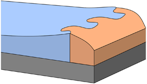
  $x_L(y,t)\leq x \leq x_N(y,t)$. As depicted in the schematic of figure 1, the thickness of fluid 2 vanishes at the leading edge and fluid 1 is supplied at constant flux in the far field (as $x\to -\infty$), which leads to a uniform thickness in the far field.

Figure 1. Schematic diagram of the profile (a) and plan view (b) of a thin film of viscous fluid of dynamic viscosity  $\mu ^{-}$ intruding into another fluid of (different) dynamic viscosity $\mu ^{+}$ down an inclined plane.
We assume that the length scale of each thin film of viscous fluid is much larger than its thickness, and that the thickness gradients may be of the order of the surface slope. We assume that the effects of inertia and surface tension are negligible and formulate a mathematical model of the flow by applying lubrication theory.
Within the limits of lubrication theory, it is the depth-averaged flux that dictates the behaviour of the flow to leading order. Integrating a parabolic velocity profile for such a flow, which satisfies no-slip at the base, yields a non-zero ( $z$-independent) velocity at all points and a non-zero flux. This may lead to a vertical front, such as the intrusion front here. Similar vertical fronts occur, for example, for lubricated viscous gravity currents, in which a thin film of viscous fluid intrudes underneath another thin film of viscous fluid of the same density (Kowal & Worster Reference Kowal and Worster2015, Reference Kowal and Worster2019b) or for thin films of a single viscous fluid down an inclined plane before being smoothed off by surface tension (Huppert Reference Huppert1982a). The former becomes unstable to a similar mechanism to that investigated here. The latter becomes unstable to a different kind of frontal instability of a wavelength chosen by a balance with surface tension.
The study most relevant to this work involves lubricated viscous gravity currents (Kowal & Worster Reference Kowal and Worster2015), which are examined both with and without a density difference. The kinematic propagation is occurring at the same time as the intrusion front becomes perpendicular to the underlying plane, while the intrusion front, as well as each vertical slice either side of the intrusion front, propagates kinematically at a rate determined locally by hydrostatic forces, which are directly associated with the upper-surface slope. That rate is the same on either side of the intrusion front, preventing the intruding fluid from overtaking the ‘pre-existing’ fluid.
A vertical force balance within the viscous gravity current upstream and downstream of the intrusion front yields a hydrostatic pressure within each viscous fluid, given by
 \begin{gather} p^{-} = \rho g \cos\theta(h-z) \quad \text{for}\ x< x_L, \end{gather}
 \begin{gather}p^{+} = \rho g \cos\theta (H-z) \quad \text{for}\ x_L< x< x_N, \end{gather}
respectively, from which it is possible to formulate and integrate (twice) the horizontal force balance, leading to the the depth-integrated flux, per unit width, given by
 \begin{gather} \boldsymbol{q^{-}}=\frac{\rho g \cos\theta}{3\mu^{-}}h^{3}(-\boldsymbol{\nabla} h + \tan\theta \boldsymbol{e}_x) \quad \text{for}\ x< x_L, \end{gather}
 \begin{gather}\boldsymbol{q^{+}}=\frac{\rho g \cos\theta}{3\mu^{+}}H^{3}(-\boldsymbol{\nabla} H + \tan\theta \boldsymbol{e}_x) \quad \text{for}\ x_L< x< x_N, \end{gather}
where  $\boldsymbol {e}_x=(1,0,0)$ and $\boldsymbol {e}_y=(0,1,0)$ are the unit basis vectors in the $x$- and $y$-directions, respectively, and the gradient operator is given by $\boldsymbol {\nabla }=({\partial }/{\partial x},\ \partial /\partial y,\ \partial /\partial z)$. The evolution of the thicknesses of both layers of fluid is determined via the mass conservation equations
 \begin{equation} \frac{\partial h}{\partial t} ={-} \boldsymbol{\nabla}\boldsymbol{\cdot} \boldsymbol{q^{-}} = \frac{\rho g\cos\theta}{3\mu^{-}}\left[ \boldsymbol{\nabla}\boldsymbol{\cdot} \left(h^{3}\boldsymbol{\nabla} h\right) - \tan\theta \frac{\partial}{\partial x}\left(h^{3}\right)\right], \end{equation}
for  $x< x_L$, and
 \begin{equation} \frac{\partial H}{\partial t} ={-} \boldsymbol{\nabla}\boldsymbol{\cdot} \boldsymbol{q^{+}} = \frac{\rho g \cos\theta}{3\mu^{+}}\left[ \boldsymbol{\nabla}\boldsymbol{\cdot} \left(H^{3}\boldsymbol{\nabla} H\right) - \tan\theta \frac{\partial}{\partial x}\left(H^{3}\right)\right], \end{equation}
for  $x_L< x< x_N$. The intruding fluid is supplied at constant flux in the far field, so that
 \begin{equation} \boldsymbol{q^{-}\cdot e_x} \to q_\infty \quad \text{as}\ x\to-\infty. \end{equation}
The normal component of the flux and the thickness of the current are both continuous across the intrusion front, so that
 \begin{equation} \boldsymbol{q^{-}\cdot n_L} = \boldsymbol{q^{+}\cdot n_L} \quad \text{at}\ x=x_L \end{equation}
and
 \begin{equation} h=H \quad \text{at}\ x=x_L, \end{equation}
where  $\boldsymbol n_L$ is the outward unit vector normal to the intrusion front $x=x_L$. The depth-integrated flux vanishes at the leading edge, giving
 \begin{equation} \boldsymbol{q^{+}\cdot n_N}=0\quad \text{at}\ x=x_N, \end{equation}
where  $\boldsymbol n_N$ is the outward unit vector normal to the leading front $x=x_N$. Equivalently, this yields the vanishing frontal thickness condition
 \begin{equation} H=0\quad \text{at}\ x=x_N. \end{equation}
A fixed volume  $V$ of fluid is released ahead of the intrusion front, so that
 \begin{equation} \int_{x_L}^{x_N} H \,\mathrm{d}\kern0.7pt x = V \end{equation}
and the leading edge  $x=x_N$ evolves kinematically, so that
 \begin{equation} \dot x_N = \lim_{x\to x_N} \frac{\boldsymbol{q\cdot n_N}}{H}. \end{equation}
Similarly, it may be deduced that
 \begin{equation} \dot x_L = \lim_{x\to x_L} \frac{\boldsymbol{q\cdot n_L}}{H}. \end{equation}
Although the last equation is redundant, we list it here for completeness.
2.1. Asymptotics near the nose
Upon inspection of the governing equations, it follows that there is a stress singularity at the nose  $x=x_N$, as a result of the diverging gradient of the thickness of the current near the nose. Such a singularity occurs also for single-layer flows (see Huppert Reference Huppert1982b), irrespective of any viscosity contrast. Near the nose, we have $|\boldsymbol {\nabla } H|\gg 1$, and so the dominant balance of the governing equation (2.6) becomes ${\partial H}/{\partial t} \sim ({\rho g \cos \theta }/{3\mu ^{+}})[ \boldsymbol {\nabla }\boldsymbol {\cdot } (H^{3}\boldsymbol {\nabla } H)],$ akin to rescaled flow over a horizontal substrate. Looking for solutions of the form $H\sim A(x_N-x)^{p}$ yields
 \begin{equation} H \sim \left[ \frac{9\mu^{+} \dot x_N}{\rho g\cos\theta} \left(1+\left(\frac{\partial x_N}{\partial y}\right)^{2}\right)^{{-}1} (x_N-x)\right]^{1/3}. \end{equation}
Similar asymptotic solutions have been obtained in the two-dimensional analyses of Huppert (Reference Huppert1982b) and Kowal & Worster (Reference Kowal and Worster2015) and the analysis of Kowal & Worster (Reference Kowal and Worster2019b), for perturbations about an axisymmetric base flow. This balance is independent of the extent of the viscous fluid ahead of the intrusion front, as well as any quantities upstream of the intrusion front.
As discussed by Mathunjwa & Hogg (Reference Mathunjwa and Hogg2006), in the context of the stability of the Barenblatt–Pattle solution, by Kowal & Worster (Reference Kowal and Worster2019a,Reference Kowal and Worsterb) in the context of the stability of lubricated viscous gravity currents, and by others, a singularity of this type poses problems when examining the linear stability of the underlying systems. As can be seen by considering small perturbations to the frontal position and linearising, the perturbed frontal thickness itself is singular. Possible remedies include transforming the dependent variable to ensure that the gradient of the new variable is non-singular (see Mathunjwa & Hogg Reference Mathunjwa and Hogg2006), adopting the method of strained coordinates (see Grundy & McLaughlin Reference Grundy and McLaughlin1982) or pinning down the front (see Kowal & Worster Reference Kowal and Worster2019a,Reference Kowal and Worsterb). We remedy this by adopting the latter approach.
2.2. Behaviour near the intrusion front
Within the limits of lubrication theory, the behaviour of the flow is driven locally by buoyancy forces, associated with a depth-averaged flux, to leading order. Any vertical shear, reflected by a parabolic velocity profile satisfying no-slip at the base, integrates to a depth-averaged ( $z$-independent) velocity, associated to a layer thickness, at each cross-section in $x$. This may lead to a flat front, such as the intrusion front at $x=x_L$, translating kinematically at the depth-averaged velocity of the layer of fluid despite any vertical shear. Physically, this may be resolved by not using lubrication theory (Goodwin & Homsy Reference Goodwin and Homsy1991) or by including the effects of surface tension (Huppert Reference Huppert1982a; Troian et al. Reference Troian, Herbolzheimer, Safran and Joann1989; Hocking Reference Hocking1990).
Similar flat fronts occur for other problems modelled using lubrication theory. Examples include the fluid–fluid intrusion front of lubricated viscous gravity currents, where a thin film of viscous fluid intrudes underneath another thin film of viscous fluid of the same density (Kowal & Worster Reference Kowal and Worster2015; Reference Kowal and Worster2019a), or the fluid–fluid intrusion front of thin films of a single viscous fluid down an inclined plane, before being smoothed off by surface tension (Huppert Reference Huppert1982a).
The former becomes unstable under a similar mechanism to that investigated here. The latter becomes unstable under a different kind of frontal instability of a wavelength chosen by a balance with surface tension.
2.3. Dimensionless equations
We note that the far-field condition (2.7) implies that the current reaches towards a steady thickness,  $h\to h_\infty$ as $x\to -\infty$, where
 \begin{equation} h_\infty = \left(\frac{3\mu^{-} q_\infty}{\rho g \sin\theta} \right)^{1/3}. \end{equation}
There is, therefore, a one-to-one mapping between the far-field flux and the far-field thickness. We scale against this thickness, and change variables as follows:
 \begin{gather} (H,h,z)= h_\infty (H^{*},h^{*},z^{*}),\quad (x,y) = (h_\infty \cot\theta) (\eta+x_N^{*},\zeta),\quad t=\left(\frac{3\mu^{-}\cos\theta}{\rho g h_\infty \sin^{2}\theta}\right)\tau, \end{gather}
 \begin{gather}(x_N,x_L) = (h_\infty \cot\theta) (x_N^{*},x_L^{*}). \end{gather}
The asterisks  $^{*}$ denote dimensionless variables. In this way, the leading front, $x=x_N$, corresponds to $\eta =0$ and the intrusion front, $x=x_L$, corresponds to $\eta =\eta _L\equiv x_L-x_N$.
After dropping asterisks, for convenience, the transformed, dimensionless fluxes reduce to
 \begin{gather} \boldsymbol{q^{-}}= h^{3}\left(-\frac{\partial h}{\partial \eta} + 1\right) \boldsymbol{e_x} + h^{3}\left( -\frac{\partial h}{\partial \zeta} + \frac{\partial x_N}{\partial \zeta}\frac{\partial h}{\partial \eta} \right) \boldsymbol{e_y} \quad \text{for}\ \eta<\eta_L, \end{gather}
 \begin{gather}\boldsymbol{q^{+}}= \mathcal{M}^{{-}1}H^{3}\left(-\frac{\partial H}{\partial \eta} + 1\right)\boldsymbol{e_x} + \mathcal{M}^{{-}1}H^{3}\left(-\frac{\partial H}{\partial \zeta} + \frac{\partial x_N}{\partial \zeta}\frac{\partial H}{\partial \eta}\right) \boldsymbol{e_y} \quad \text{for}\ \eta>\eta_L. \end{gather}
The governing mass conservation equations become
 \begin{gather} \frac{\partial h}{\partial \tau} - \dot x_N \frac{\partial h}{\partial \eta} ={-} \frac{\partial}{\partial \eta} \left(q^{-}_x\right) - \left( \frac{\partial}{\partial \zeta} - \frac{\partial x_N}{\partial \zeta}\frac{\partial}{\partial \eta} \right) \left( q^{-}_y\right), \quad \text{for}\ \eta<\eta_L, \end{gather}
 \begin{gather}\frac{\partial H}{\partial \tau} - \dot x_N \frac{\partial H}{\partial \eta} ={-} \frac{\partial}{\partial \eta} \left(q^{+}_x\right) - \left( \frac{\partial}{\partial \zeta} - \frac{\partial x_N}{\partial \zeta}\frac{\partial}{\partial \eta} \right) \left( q^{+}_y\right) \quad \text{for}\ \eta>\eta_L, \end{gather}
where the subscripts  $_x$ and $_y$ denote the $x$ and $y$ vector components, respectively, and the overdot denotes partial differentiation with respect to $\tau$. Similarly, the boundary conditions become
 \begin{gather} q^{-}_x \to 1 \quad \text{as}\ \eta\to-\infty, \end{gather}
 \begin{gather}q^{-}_x - \left( \frac{\partial x_L}{\partial \zeta} \right) q^{-}_y= q^{+}_x - \left( \frac{\partial x_L}{\partial \zeta} \right) q^{+}_y \quad \text{at}\ \eta=\eta_L, \end{gather}
 \begin{gather}h=H \quad \text{at}\ \eta=\eta_L, \end{gather}
 \begin{gather}H=0 \quad \text{at}\ \eta=0. \end{gather}
The global mass conservation condition reduces to
 \begin{equation} \int_{\eta_L}^{0} H \,\mathrm{d}\eta = \mathcal{V} \end{equation}
and the kinematic condition reduces to
 \begin{equation} \dot x_N = \lim_{\eta\to 0} H^{{-}1}\left(q^{+}_x - \frac{\partial x_N}{\partial \zeta}q^{+}_y\right) \left( 1 + \left( \frac{\partial x_N}{\partial \zeta} \right)^{2} \right)^{{-}1/2}. \end{equation}
It is not necessary to use a kinematic condition for the intrusion front  $x_L$, as the global condition (2.27) is sufficient to specify $x_L$.
The asymptotic solution near the leading front is given, in dimensionless form, by
 \begin{equation} H \sim \left[- 3\mathcal{M} \dot x_N \eta \left(1+\left(\frac{\partial x_N}{\partial \zeta}\right)^{2}\right)^{{-}1}\right]^{1/3} \quad \text{as}\ \eta\to 0^{-}. \end{equation}
The solutions are determined by two dimensionless parameters: the viscosity ratio  $\mathcal {M}$ and the fixed volume $\mathcal {V}$ of viscous fluid ahead of the intrusion front. Explicitly, these dimensionless parameters are given by
 \begin{equation} \mathcal{M}=\frac{\mu^{+}}{\mu^{-}}, \quad \text{and} \quad \mathcal{V}=\frac{V\tan\theta}{h^{2}_\infty}. \end{equation}
2.4. Travelling-wave solution
The basic state, which we wish to perturb to examine its stability, takes the form of a  $y$-independent travelling-wave solution $\boldsymbol {\varPsi }_0=(h_0(\eta ),\ H_0(\eta ),\ \eta _{L0},\ x_{N0})$ of unit speed in the frame of the advancing front. Here, the subscript $_0$ refers to quantities corresponding to the basic state. Without loss of generality, the origin is set to coincide with the leading front of the current, so that $\eta =\eta _{N0}=0$ corresponds to $x=x_{N0}$. As the travelling-wave solution is of unit speed (equal to the far-field speed), both fronts evolve as $\dot x_{N0}=\dot x_{L0}=1$, so that $x_{N0}=\tau$ and $x_{L0}=\tau +\eta _{L0}$. That is, the velocity of the travelling-wave solution is determined fully by the upstream, far-field flux.
The depth-integrated fluxes per unit width reduce to
 \begin{gather} q^{-}_0=h_0^{3} \left(1-h_0'\right) \quad \text{for}\ \eta<\eta_{L0}, \end{gather}
 \begin{gather}q^{+}_0={\mathcal{M}}^{{-}1}H_0^{3} \left(1-H_0'\right) \quad \text{for}\ \eta_{L0}<\eta<0, \end{gather}
where the prime  $^{\prime }$ denotes differentiation with respect to $\eta$. After a further integration in $\eta$ and simplification, the governing equations in the two regions reduce to
 \begin{gather} h_0^{2} \left(1-h_0'\right)=1 \quad \text{for}\ \eta<\eta_{L0}, \end{gather}
 \begin{gather}{\mathcal{M}}^{{-}1}H_0^{2} \left(1-H_0'\right)=1 \quad \text{for}\ \eta_{L0}<\eta<0, \end{gather}
subject to the boundary conditions
 \begin{gather} q^{-}_0 \to 1 \quad \text{as}\ \eta\to-\infty, \end{gather}
 \begin{gather}h_0=H_0 \quad \text{at}\ \eta=\eta_{L0}, \end{gather}
 \begin{gather}q^{-}_0=q^{+}_0 \quad \text{at}\ \eta=\eta_{L0}, \end{gather}
 \begin{gather}H_0=0 \quad \text{at}\ \eta=0 \end{gather}
and the global mass conservation condition
 \begin{equation} \int_{\eta_{L0}}^{0} H_0 \,\mathrm{d}\eta=\mathcal{V}. \end{equation}
The travelling-wave solution retains the inherent cube-root singularity near the leading front, of the form
 \begin{equation} H_0 \sim \left(- 3\mathcal{M} \eta \right)^{1/3} \quad \text{as}\ \eta\to 0^{-}. \end{equation}
After a further integration of the governing equations in  $\eta$, it can be seen that there is an analytic solution, given implicitly by
 \begin{gather} h_0+\frac{1}{2} \log \left|\frac{ h_0-1 }{ h_0+1 }\right| = \eta -\eta_a, \quad \text{for}\ \eta<\eta_{L0}, \end{gather}
 \begin{gather}H_0+\frac{\sqrt{\mathcal{M}}}{2} \log \left|\frac{ H_0-\sqrt{\mathcal{M}} }{ H_0+\sqrt{\mathcal{M}} }\right| = \eta -\eta_b, \quad \text{for}\ \eta_{L0}<\eta<0. \end{gather}
By applying the vanishing thickness condition (2.38), we find  $\eta _b$=0. There are no explicit formulas for the constants $\eta _a$ and $\eta _{L0}$. These can be determined implicitly by applying the global mass balance (2.39) and the thickness continuity condition (2.36).
Two limiting cases are worth noting: the limits of  $\mathcal {V}=0$ and $\mathcal {V}\to \infty$. Both of these describe the flow of a single layer of fluid of the corresponding viscosity. In the limit of $\mathcal {V}=0$, the governing equations and boundary conditions reduce to
 $$\begin{gather} h_0^{2} \left(1-h_0'\right)=1 \quad \text{for}\ \eta<0, \end{gather}$$
 $$\begin{gather}h_0^{3} \left(1-h_0'\right)\to 1\quad \text{as}\ \eta\to-\infty,\quad h_0=0 \quad\text{at}\ \eta=0, \end{gather}$$
with an analytic solution given implicitly by
 \begin{equation} h_0+\frac{1}{2} \log \left|\frac{ h_0-1 }{ h_0+1 }\right| = \eta, \quad \text{for}\ \eta<0. \end{equation}
In the limit of  $\mathcal {V}\to \infty$, the governing equations and boundary conditions reduce to
 \begin{gather} \mathcal{M}^{{-}1}H_0^{2} \left(1-H_0'\right)=1 \quad \text{for}\ \eta<0, \end{gather}
 \begin{gather}\mathcal{M}^{{-}1}H_0^{3} \left(1-H_0'\right)\to 1\quad \text{as}\ \eta\to-\infty,\quad H_0=0 \quad\text{at } \eta=0, \end{gather}
with an analytic solution given implicitly by
 \begin{equation} H_0+\frac{\sqrt{\mathcal{M}}}{2} \log \left|\frac{ H_0-\sqrt{\mathcal{M}} }{ H_0+\sqrt{\mathcal{M}} }\right| = \eta, \quad \text{for}\ \eta<0. \end{equation}
 Illustrative solutions for sample parameter values are shown in figure 2, along with the  $\mathcal {V}=0$ and $\mathcal {V}\to \infty$ limiting solutions, and the solution for $-\eta _{L0}$ is shown in figure 3. The solutions are enveloped by the limiting solutions at fixed $\mathcal {M}$. The solution for which ${\mathcal {M}=1}$ corresponds to a classical viscous gravity current of uniform viscosity down an inclined plane. In such a scenario, the viscous fluids to the left and to the right of the intrusion front are identical. The scenario in which $\mathcal {M}>1$ corresponds to a less viscous fluid intruding into a more viscous fluid. In this scenario, the upper-surface slope is discontinuous at the intrusion front. The greater the viscosity ratio, the greater the jump in slope. Such a change in slope corresponds to a change in hydrostatic pressure gradient, as can be deduced from the pressure fields (2.1) and (2.2). The mechanism of instability is directly related to such a jump in hydrostatic pressure gradient, as explained in § 4.

Figure 2. (a) Base-flow solution for a range of values of the viscosity ratio  $\mathcal {M}$ and $\mathcal {V}=1$. The jump in upper-surface slope (hence, in the pressure gradient) at the intrusion front increases for increasing viscosity ratios. (b) Base-flow solution for a range of values of $\mathcal {V}$ for $\mathcal {M}=5$. The $\mathcal {V}=0$ limit is shown as a dashed curve and the $\mathcal {V}\to \infty$ limit is shown as a dotted curve.

Figure 3. The extent  $-\eta _{L0}$ as a function of the viscosity ratio $\mathcal {M}$ for $\mathcal {V}=1$ (a) and as a function of the volume $\mathcal {V}$ for $\mathcal {M}=2$ (b) on logarithmically scaled axes.
It is worth noting that although the slope discontinuity at the intrusion front may become large in the limits of  $\mathcal {M}\to \infty$ or $\mathcal {V}\to \infty$, the upstream upper-surface slope is never positive with respect to the horizontal. This can be seen by solving (2.33) for $h_0'$, which gives $h_0' = 1-1/h_0^{2}\leq 1$. That is, whatever the value of the parameters, the upper-surface slope is smaller than 0 at all points (measuring the slope in coordinates aligned with the horizontal and vertical). This means that the slope does not become positive (with respect to the horizontal), so the depth-integrated flow, and hence the intrusion front, does not travel upwards. Alternatively, this conclusion can be reached by considering the upstream flux as given by (2.31), which is always positive.
3. Perturbations
We examine the stability of the problem by perturbing about the travelling-wave solution of § 2.4, and searching for normal modes of the form
 \begin{equation} \boldsymbol{\varPsi}(\eta,\zeta,\tau) = \boldsymbol{\varPsi}_0(\eta) + \epsilon \boldsymbol{\varPsi}_1(\eta)\exp(\sigma \tau + \textrm{i} k \zeta),\end{equation}
where
 \begin{gather} \boldsymbol{\varPsi}(\eta,\zeta,\tau) = \left(h(\eta,\zeta,\tau), H(\eta,\zeta,\tau),\eta_{L}(\zeta,\tau),x_{N}(\zeta,\tau)\right), \end{gather}
 \begin{gather}\boldsymbol{\varPsi}_0(\eta) = \left(h_0(\eta), H_0(\eta),\eta_{L0},x_{N0}\right), \end{gather}
 \begin{gather}\boldsymbol{\varPsi}_1(\eta) = \left(h_1(\eta), H_1(\eta),\eta_{L1},x_{N1}\right). \end{gather}
Note that the  $\tau$ and $\zeta$ dependence of the perturbations are factored into the $\exp (\sigma \tau +\textrm {i}k\zeta )$ term of (3.1). Here, $\epsilon$ is a small parameter denoting the order of magnitude of the perturbed quantities. We wish to expand in $\epsilon$ to obtain the governing equations, and the boundary, integral and kinematic conditions for the perturbations at first order in $\epsilon$. These will form a system of linear differential equations in $\eta$, which admit the normal mode solutions of the form (3.1).
At first order in  $\epsilon$, the perturbations to the fluxes reduce to
 \begin{equation} \boldsymbol{q_1^{-}} = \left(3h_0^{2}h_1-h_0^{3} h_1'-3h_0^{2}h_1h_0'\right) \boldsymbol{e_x} + \textrm{i} k h_0^{3}\left( x_{N1}h_0' -h_1 \right)\boldsymbol{e_y}, \end{equation}
for  $\eta <\eta _{L0}$, and
 \begin{equation} \boldsymbol{q_1^{+}} = \mathcal{M}^{{-}1}\left[ \left(3H_0^{2}H_1-H_0^{3} H_1'-3H_0^{2}H_1H_0' \right) \boldsymbol{e_x} + \textrm{i} k H_0^{3}\left( x_{N1}H_0' -H_1 \right)\boldsymbol{e_y} \right], \end{equation}
for  $\eta _{L0}<\eta <0$. The governing equations become
 \begin{equation} \sigma h_1 - h_1' - \sigma x_{N1} h_0' =\left( h_0^{3}h_1' + 3h_0^{2}h_1h_0'-3h_0^{2}h_1\right)' - k^{2} h_0^{3}\left(h_1 - x_{N1}h_0'\right), \end{equation}
for  $\eta <\eta _{L0}$, and
 \begin{align} & \sigma H_1 - H_1' - \sigma x_{N1} H_0' \nonumber\\ &\quad =\mathcal{M}^{{-}1}\left[\left( H_0^{3} H_1' + 3 H_0^{2} H_1 H_0'-3H_0^{2} H_1\right)' - k^{2} H_0^{3}\left(H_1 - x_{N1}H_0'\right)\right], \end{align}
for  $\eta _{L0}<\eta <0$. The boundary conditions for the perturbations reduce to
 \begin{gather} q_{1x}^{-} \to 0 \quad \text{as}\ \eta\to-\infty, \end{gather}
 \begin{gather}h_1 +\eta_{L1} h_0' = H_1 +\eta_{L1} H_0' \quad \text{at}\ \eta=\eta_{L0}, \end{gather}
 \begin{gather}q_{1x}^{-} + \eta_{L1} \left(q_{0x}^{-}\right)' = q_{1x}^{+} + \eta_{L1} \left(q_{0x}^{+}\right)' \quad \text{at}\ \eta=\eta_{L0}, \end{gather}
 \begin{gather}H_1=0 \quad \text{at}\ \eta=0. \end{gather}
Note that it is exponential growth in  $t$, rather than in $\eta$, that determines stability. As such, although the condition that the perturbation flux vanishes as $\eta \to -\infty$ results in eigenmodes that vanish in the far field, there may well be growth near the intrusion front. That is, the boundary condition that the flux vanishes as $\eta \to -\infty$ does not preclude exponential growth in $t$ near the intrusion front. See Kowal & Worster (Reference Kowal and Worster2019a) for a similar phenomenon.
In contrast to viscous fingering in a porous medium, which is most conveniently explained in terms of associated potentials, the fingering instability examined here is described in terms of depth-averaged fluxes, which depend on the deflection of the upper surface. These, in turn, need to be determined as part of the system of nonlinear differential equations (3.5)–(3.12) describing a local mass balance. Owing to the  $\mathcal {M}^{-1}$ prefactor associated with the depth-integrated upstream flux (3.6), higher upstream hydrostatic pressure gradients are necessary to drive the upstream flow if $\mathcal {M}>1$ to preserve continuity of flux (3.11). As such, if a parcel of intruding fluid is perturbed ahead of the initially planar intrusion front, it becomes subject to higher hydrostatic pressure gradients, advancing further downstream.
The global mass balance for the perturbations becomes
 \begin{equation} \left.\int_{\eta_{L0}}^{0} H_1 \,\mathrm{d}\eta = \eta_{L1} H_0\right|_{\eta=\eta_{L0}}, \end{equation}
the kinematic condition for perturbations to the frontal position reduces to
 \begin{equation} \sigma x_{N1} = \lim_{\eta\to 0} \left( \frac{q_{1x}^{+}}{H_0} - \frac{q_{0x}^{+}H_1}{H_0^{2}}\right), \end{equation}
and the asymptotic solution near the front becomes
 \begin{equation} H_1 \sim \tfrac{1}{3}\sigma x_{N1} \left(- 3\mathcal{M} \eta \right)^{1/3} \quad \text{as}\ \eta\to 0^{-}, \end{equation}
which does not diverge as  $\eta \to 0^{-}$.
3.1. Numerical solutions
The system of equations specified in the previous section forms a complete set of governing equations, and boundary, integral and kinematic conditions to specify the perturbations as the solution to a nonlinear eigenvalue problem, for which the growth rate  $\sigma$ acts as the eigenvalue. We note that by the linearity of this system of differential equations, any multiple of a solution $(h_1, H_1, \eta _{L1}, x_{N1})$ is also a solution. We, therefore, set $x_{N1}=1$, without loss of generality. This condition forms a nonlinear equation
 \begin{equation} f(\sigma,k,\mathcal{M},\mathcal{V})=0, \end{equation}
which implicitly determines the growth rate  $\sigma$ as a function of the wavenumber $k$, viscosity ratio $\mathcal {M}$ and volume $\mathcal {V}$.
Numerically, these equations are solved on the interval  $(-L,\eta _{L0})$, approximating the semi-infinite interval $(-\infty ,\eta _{L0})$ and corresponding to the intruding fluid, and on the interval $(\eta _{L0},\delta )$, approximating the full interval $(\eta _{L0},0)$ including the singular nose and corresponding to the viscous fluid ahead of the intrusion front. This has been achieved using Mathematica's built-in numerical solver for differential equations. Here, $L$ is taken to be a large, finite and positive number, and $\delta$ is taken to be small positive number.
Introducing the non-zero parameter  $\delta$ serves as a way to avoid numerical instabilities near the singularity at the nose. The equations are discretised on the interval $(\eta _{L0},\delta )$, with boundary conditions applied at $\eta =\delta$ using the asymptotic solution (3.15).
Another source of numerical error originates from the far-field behaviour of the general solution for the perturbations in the limit  $\eta \to -\infty$. Specifically, although the desired solution satisfying the far-field condition decays as $\eta \to -\infty$, we find that the general solution for the perturbations consists of a linear combination of terms, one of which grows exponentially for growth rates of interest, specifically when $\sigma >-k^{2}$, as
 \begin{equation} h_1 \sim c \exp\left(\left(1-\sqrt{1+k^{2}+\sigma}\right)\eta\right) \quad \text{as}\ \eta\to-\infty \end{equation}
for some constant  $c$. To ensure numerical stability we solve for the transformed variable $g_1$ instead of $h_1$, where
 \begin{equation} g_1(\eta) \equiv h_1(\eta) \exp\left(-\left(1-\sqrt{1+k^{2}+\sigma}\right)\eta\right) \end{equation}
and apply the far-field boundary condition in terms of  $g_1$. In this way, $g_1$ remains finite as $\eta \to -\infty$.
4. Mechanism of instability
In contrast to widely known viscous fingering instabilities in porous media, which are driven by a change in dynamic pressure gradient across the intrusion front, viscous fingering instabilities may also occur in unconfined environments, such as in the free-surface flow considered in this paper. These instabilities are instead driven by a change in hydrostatic pressure gradient across the intrusion front, and are stabilised by buoyancy forces at large wavenumbers. A necessary, though insufficient, condition for instability is that the intruding fluid be less viscous than the fluid ahead of the intrusion front, that is,  $\mathcal {M} > 1$.
This can be understood by considering the dimensionless longitudinal pressure gradient
 \begin{gather} G_0^{-}= (p_0^{-})' = h_0' \quad \text{for}\ \eta<\eta_L, \end{gather}
 \begin{gather}G_0^{+}= (p_0^{+})' = H_0' \quad \text{for}\ \eta_L<\eta<\eta_N \end{gather}
of the base flow, made dimensionless by scaling the pressure using the scale  $\rho g h_\infty \cos \theta$. As a consequence of the conditions of continuity of thickness (2.36) and flux (2.37), the jump in hydrostatic pressure gradient,
 \begin{equation} [G_0]^{+}_-= \left(\mathcal{M}-1\right) \left(G_0^{-} -1\right), \end{equation}
changes sign when  $\mathcal {M}=1$. Noting that $G_0^{-} <1$ (as can be seen by solving (2.33) for $h_0'$), it follows that when the intruding fluid, upstream of the intrusion front, is less viscous than the viscous fluid ahead of the intrusion front ( $\mathcal {M}>1$), there is a jump in the hydrostatic pressure gradient across the intrusion front so that $-[G_0]^{+}_->0$. That is, the negative pressure gradient downstream of the intrusion front exceeds its upstream value. As a parcel of less viscous fluid gets perturbed ahead of the intrusion front, it becomes subject to a steeper hydrostatic pressure gradient, which advances it further away from the intrusion front. The jump $-[G_0]^{+}_-$ versus $\mathcal {M}$ is shown in figure 4, showing that $-[G_0]^{+}_->0$ for $\mathcal {M}>1$.

Figure 4. (a) The jump in pressure gradient  $-[G_0]^{+}_-$ across the intrusion front versus the viscosity ratio for various values of $\mathcal {V}$. (b) The rate of work done in deforming the upper surface just to the left (dashed) and right (solid) of the intrusion front as a function of $\mathcal {M}$ for $\mathcal {V}=1$.
If, on the other hand, the intruding fluid is more viscous than the viscous fluid ahead of the intrusion front ( $\mathcal {M}<1$) and the upstream pressure force exceeds buoyancy forces ( $G_0^{-} >1$), then the pressure gradient downstream of the intrusion front is smaller than the upstream pressure gradient. As a parcel of more viscous fluid gets perturbed ahead of the intrusion front, it becomes subject to a lower hydrostatic pressure gradient and does not advance further away from the intrusion front.
It is also illuminating to think of the instability mechanism from an energy perspective. Out of the various contributions to the right-hand side of the equation of conservation of energy, the ones of interest for this flow include the rate of work done in deforming the upper surface, and the local stress working, owing to viscous dissipation. These two contributions are dominant also for other viscosity-induced interfacial instabilities of thin-film flows, as outlined by Boomkamp & Miesen (Reference Boomkamp and Miesen1997). The former, which are given by  $\varPhi ^{-}=h_0h_1(\frac {1}{2}h_0h_1'+h_1(h_0'-1))(h_0'-1)$ for the intruding layer and $\varPhi ^{+}=({1}/{\mathcal {M}})H_0H_1(\frac {1}{2}H_0H_1'+H_1(H_0'-1))(H_0'-1)$ ahead of the intrusion front, per unit area, are largest near the intrusion front and its values at the intrusion front increase with the viscosity ratio $\mathcal {M}$, as seen in figure 4. Both of these are proportional to the upper-surface slope minus the slope of the inclined substrate, over which the two fluids propagate. Equivalently, these are proportional to the upstream and downstream pressure forces, in excess of downslope gravitational forces. As already discussed, a greater imbalance of these across the intrusion front leads to a greater instability. This is consistent with numerical results, where greater values of $\mathcal {M}$ lead to greater instabilities.
The mechanism is similar to the instability found in the experiments of Kowal & Worster (Reference Kowal and Worster2015) of lubricated viscous gravity currents, explained in the stability analyses of Kowal & Worster (Reference Kowal and Worster2019a,Reference Kowal and Worsterb) in various limits. In the context of lubricated viscous gravity currents, the instability is also driven by a jump in hydrostatic pressure gradient; however, no additional longitudinal buoyancy forces act as a stabilising mechanism. As pointed out earlier, the mechanism of instability is also similar to that of classical viscous fingering instabilities in porous media, but is driven by a hydrostatic, rather than dynamic, pressure gradient. This is what highlights the main difference between the instability considered here and classical viscous fingering instabilities.
5. Discussion of results
As discussed in the previous section, instability occurs as a result of a jump in hydrostatic pressure gradient at the intrusion front and a necessary condition for instability is  ${\mathcal {M}>1}$. However, $\mathcal {M}>1$ is not a sufficient condition owing to additional buoyancy forces acting as a stabilising mechanism. This section presents a discussion of numerical results illustrating the instability in parameter space.
As illustrated in figure 5, the instability occurs within a band of unstable wavenumbers bounded by  $k=0$ and the cut-off wavenumber $k=k_0$, defined as the wavenumber at which $\sigma =0$. The growth rates increase and the band of unstable wavenumbers expands with increasing viscosity ratios $\mathcal {M}$ and decreasing frontal volume $\mathcal {V}$ up to a threshold. The instability diminishes for both $\mathcal {V}\ll 1$ and $\mathcal {V}\gg 1$.

Figure 5. Growth rate  $\sigma$ as a function of the wavenumber $k$ for a range of values of $\mathcal {V}$ (a,b) and $\mathcal {M}$ (c). (a) $\mathcal {M}=5$ and $\mathcal {V}=0.1$, $0.2$, $0.3$, $0.4$, $0.5$. (b) $\mathcal {M}=5$ and $\mathcal {V}=1$, $2$,
$2$,  $3$,
$3$,  $4$,
$4$,  $5$. (c) $\mathcal {M}=3$, $4$,
$4$,  $\dots ,$ $10$ and $\mathcal {V}=1$.
Such behaviour is also reflected in plots of the cut-off wavenumber as a function of  $\mathcal {M}$ and $\mathcal {V}$ in figures 6 and 7. The critical wavenumber, defined as the wavenumber for which the growth rate is maximal, is also shown in these figures. In contrast to the cut-off wavenumber, the critical wavenumber initially increases, reaches a peak and then decreases with $\mathcal {M}$ as shown in figure 7.

Figure 6. Critical wavenumber  $k_c$ (a) and cut-off wavenumber $k_0$ (b) versus $\mathcal {V}$ for a range of values of $\mathcal {M}$.

Figure 7. Critical wavenumber  $k_c$ (a) and cut-off wavenumber $k_0$ (b) versus $\mathcal {M}$ for a range of values of $\mathcal {V}>1$.
As seen in figures 6 and 7, a distinguishing feature between variations in  $\mathcal {M}$ and variations in $\mathcal {V}$ is that the instability occurs in bounded intervals of $\mathcal {V}$ and semi-infinite intervals of $\mathcal {M}$. This is because the instability persists for arbitrarily large values of $\mathcal {M}$, as the jump in hydrostatic pressure gradient across the intrusion front increases as $\mathcal {M}\to \infty$. The bigger the viscosity ratio, the bigger the window of instability. However, large or small values of $\mathcal {V}$ are stabilising as seen in figure 6.
Physically, large and small values of  $\mathcal {V}$ correspond to the single-fluid limit of a thin film of a single fluid spreading under gravity, which, in the absence of surface tension, leads to stability. For example, the small $\mathcal {V}$ limit corresponds to the two-dimensional flows of Huppert (Reference Huppert1982b), which are known to be stable (Mathunjwa & Hogg Reference Mathunjwa and Hogg2006). Buoyancy forces stabilise the system in these limits. Similar behaviour is found here: as either the large- $\mathcal {V}$ or the small- $\mathcal {V}$ limits are approached, the instability diminishes.
The approach towards these two limits is seen in figures 7 and 8. The critical wavenumber and the cut-off wavenumber are shown as functions of  $\mathcal {M}$ for a range of values of $\mathcal {V}$, where $\mathcal {V}$ is large in figure 7 and small in figure 8. It can be seen in figure 7 that the minimal viscosity ratio required for the onset of instability increases with $\mathcal {V}$ when $\mathcal {V}$ is large; this is consistent with the expectation that the instability diminishes in the large- $\mathcal {V}$ limit. The opposite behaviour occurs near the small- $\mathcal {V}$ limit. It can be seen in figure 8 that the minimal viscosity ratio required for the onset of instability increases with decreasing $\mathcal {V}$ when $\mathcal {V}$ is small; this is consistent with the expectation that the instability diminishes in the small- $\mathcal {V}$ limit. The instability is most prevalent for intermediate values of $\mathcal {V}$.

Figure 8. Critical wavenumber  $k_c$ (a) and cut-off wavenumber $k_0$ (b) versus $\mathcal {M}$ for a range of values of $\mathcal {V}\ll 1$.
A similar conclusion, in terms of the magnitude of the growth rate, can be reached by reflecting upon the results of figure 9. Figure 9 shows the critical, or maximal, growth rate  $\sigma _c$ as a function of $\mathcal {M}$ for a range of values of $\mathcal {V}$ near both the large- $\mathcal {V}$ limit and the small- $\mathcal {V}$ limit. The growth rate of the instability is seen to decrease towards the large- $\mathcal {V}$ and small- $\mathcal {V}$ limits. In contrast, the growth rates increase indefinitely for increasing viscosity ratios, and the instability is suppressed completely for viscosity ratios lower than about $\mathcal {M}\approx 2$ (more precisely, $\mathcal {M}\approx 1.97$), as seen in figure 10. As observed similarly before, a distinguishing feature between variations in $\mathcal {V}$ and variations in $\mathcal {M}$ is that any given growth rate is seen only in a bounded interval of $\mathcal {V}$.

Figure 9. Critical growth rate  $\sigma _c$ versus $\mathcal {M}$ for a range of values of $\mathcal {V}>1$ (a) and $\mathcal {V}\ll 1$ (b).

Figure 10. Critical growth rate  $\sigma _c$ versus $\mathcal {V}$ for a range of values of $\mathcal {M}$.
Several neutral curves, depicting the value of  $\mathcal {M}=\mathcal {M}_n$ for which $\sigma =0$, are shown in figure 11 for a range of values of $\mathcal {V}$. As expected, the neutral curves shift upwards as $\mathcal {V}$ increases. Increasingly large viscosity ratios are required for any instability to occur as $\mathcal {V}$ increases. The minimal viscosity ratio required for the onset of instability occurs at $k=0$, reflecting that small wavenumbers are seen first as the viscosity ratio increases towards its neutral value. Higher wavenumbers, with a non-zero critical wavenumber $k=k_c$ at which the growth rate is maximal, are seen above the neutral threshold for $\mathcal {M}$.

Figure 11. Neutral curves for the viscosity ratio versus the wavenumber for a range of values of  $\mathcal {V}$.
All of the aforementioned information on regions of instability can be collated into a single stability diagram in figure 12, displaying regions of stability and instability in  $(\mathcal {M}, \mathcal {V})$ space. As discussed at the beginning of this section, $\mathcal {M}>1$ is a necessary but not sufficient condition for instability. Higher viscosity ratios are in fact necessary and sufficient for an instability to occur. The minimal viscosity ratio required is approximately $\mathcal {M}\approx 1.97$, which gives rise to instability as long as $\mathcal {V}\approx 0.92$. The band of values of $\mathcal {V}$ for which an instability occurs widens as $\mathcal {M}$ increases away from $\mathcal {M}\approx 1.97$. However, this band of values is always bounded, for any given value of $\mathcal {M}$ above the threshold; this is consistent with the stabilisation in the small- $\mathcal {V}$ and large- $\mathcal {V}$ limits.

Figure 12. Stability diagram in  $(\mathcal {V}, \mathcal {M})$ space. The axes are scaled logarithmically. Instabilities occur when the viscostiy ratio $\mathcal {M}$ is sufficiently large. Power laws for the $\mathcal {V}\ll 1$ and $\mathcal {V}\gg 1$ limits are shown as dashed lines. Small or large volumes $\mathcal {V}$ require a larger viscosity contrast to trigger an instability.
A linear fit to logarithmically scaled data shows that the neutral curve follows the approximate form  $\mathcal {M}\sim 1.59 \mathcal {V}^{0.51}$ as $\mathcal {V}\to \infty$, and $\mathcal {M}\sim 0.29 \mathcal {V}^{-0.98}$ as $\mathcal {V}\to 0$. The large $\mathcal {V}$ result can be deduced by noting that $h_0$ and $H_0$ scale as $\sqrt {\mathcal {M}}$ at $\eta =\eta _{L0}$ for $\mathcal {V}\gg 1$, from the far-field limit of (2.42), and $\eta _{L0}$ scales as $-\mathcal {V}/\sqrt {\mathcal {M}}$, to satisfy the global mass constraint (2.39). As such, the downstream pressure gradient scales as $\mathcal {M}/\mathcal {V}$. Balancing this against the upstream pressure gradient, on the order of $h_0^{2}\sim 1/\mathcal {M}$, in excess of downslope gravitational forces, yields that $\mathcal {M}$ scales as $\mathcal {V}^{1/2}$ (cf. the numerically obtained result $\mathcal {M}\sim 1.59 \mathcal {V}^{0.51}$ for $\mathcal {V}\gg 1$). The small $\mathcal {V}$ result can be deduced by noting that the asymptotic solution (2.40) applies throughout the region ahead of the intrusion front. Consistently with the global mass condition (2.39), the extent beyond the intrusion front scales as $\mathcal {V}^{3/4}\mathcal {M}^{-1/4}$ and the thickness at the intrusion front scales as $(\mathcal {MV})^{1/4}$, whereas the far-field upstream thickness reaches $h_0\sim 1$. A sufficiently high upstream pressure gradient is maintained when these are balanced ( $H_{0}\sim 1$) so that $(\mathcal {MV})^{1/4}$ is of order unity. This occurs when $\mathcal {M}$ scales with $\mathcal {V}^{-1}$ (cf. the numerically obtained result $\mathcal {M}\sim 0.29 \mathcal {V}^{-0.98}$ for $\mathcal {V}\ll 1$).
6. Conclusions
We have demonstrated that viscous fingering instabilities, originally discovered within porous media in the seminal work of Saffman & Taylor (Reference Saffman and Taylor1958), are also present in other, non-porous environments. An example is the free-surface flow considered in this paper. Although the mechanism of instability is fundamentally different, there are important similarities between non-porous viscous fingering instabilities of the free-surface flow of a thin film of viscous fluid intruding into a more viscous fluid, and Saffman–Taylor viscous fingering instabilities in porous media.
Physically, both viscous fingering instabilities originate from a jump in pressure gradient across the intrusion front. The difference is that the pressure field is hydrostatic in the context of non-porous viscous fingering instabilities, and dynamic in the context of Saffman–Taylor instabilities in porous media.
In a porous medium, the interface between two viscous fluids of differing viscosities is unstable under small perturbations if the intruding fluid is less viscous than the ambient fluid. Symbolically, this occurs when the viscosity ratio  $\mathcal {M}$ between the two viscous fluids is greater than 1. In the free-surface flow considered in this paper, the condition $\mathcal {M}>1$ is a necessary but not sufficient condition for instability as there is the additional stabilising influence of longitudinal gravitational forces. In fact, a viscosity ratio of at least $\mathcal {M}\gtrapprox 2$ is required for instability. Instabilities occur in the vicinity of this stability threshold as long as the dimensionless volume of viscous fluid ahead of the intrusion front is approximately $\mathcal {V}\approx 0.9$.
Beyond this stability threshold, the band of values of  $\mathcal {V}$ for which instability occurs widens with increasing viscosity ratios, but remains bounded from above and from below. Physically, the upper and lower bounds result from the dominance of stabilising longitudinal buoyancy forces for large and small volumes $\mathcal {V}$. The limits of $\mathcal {V}\to \infty$ and $\mathcal {V}\to 0$ correspond to a thin film of a single viscous fluid flowing down a slope, of either the smaller or the larger viscosity.
The critical wavenumber  $k=k_c$ selected by the system as the most unstable wavenumber depends upon the balance between the destabilising jump in hydrostatic pressure gradient and the stabilising influence of buoyancy forces. This balance depends upon the viscosity ratio $\mathcal {M}$ and volume $\mathcal {V}$. The largest critical wavenumbers occur for the combination of large values of $\mathcal {M}$ and small values of $\mathcal {V}$. Small critical wavenumbers are most prevalent for small viscosity ratios $\mathcal {M}$ and moderate volumes $\mathcal {V}$. Large values of $\mathcal {V}$ lead to smaller critical wavenumbers and require a larger viscosity ratio in order for any instability to occur. Similar behaviour is found for small $\mathcal {V}$.
Funding
This work was partially funded by L'Oréal-UNESCO UK and Ireland, For Women In Science (FWIS).
Declaration of interests
The author reports no conflict of interest.


 Open access