


1. Introduction
On 15 January 2022 the Hunga Tonga Hunga Ha'apai volcano erupted violently in the South Pacific (hereafter referred to as the ‘Tonga event’) after a month of volcanic activity, triggering tsunamis that reached coasts around the Pacific rim and ‘exposed a blind spot in Japan's tsunami monitoring and warning system’ (Imamura et al. Reference Imamura, Suppasri, Arikawa, Koshimura, Satake and Tanioka2022). Japan's warning system disregarded ocean surface perturbations induced by the atmospheric pressure waves generated by the eruption, delaying the evacuation process in the Amami Islands (Imamura et al. Reference Imamura, Suppasri, Arikawa, Koshimura, Satake and Tanioka2022). This lack of understanding of the mechanisms behind the generated tsunami has prompted the authors to investigate the matter. The eruption is one of the largest recorded in modern times and has been compared with the eruption of Krakatoa in 1883 (Matoza Reference Matoza2022). Energy was released by the eruption into the atmosphere, ocean and ground. It generated acoustic, gravity and seismic waves that were detected by an array of instruments around the globe (Matoza Reference Matoza2022; Vergoz et al. Reference Vergoz2022; Wright et al. Reference Wright2022), producing an abundance of available data for the study of the event. Infrasound stations, weather satellites and ground weather stations recorded atmospheric pressure disturbances propagating from Tonga to its antipode and back, in cycles of around 36 hrs, for more than seven days (Díaz & Rigby Reference Díaz and Rigby2022; Kulichkov et al. Reference Kulichkov2022; Otsuka Reference Otsuka2022; Yuen et al. Reference Yuen2022). Figure 1 shows the thermal signature of the atmospheric pressure waves for the 9.6  $\mathrm {\mu }$m centred infrared (IR) band captured by geostationary weather satellites. Different spectral bands, each most sensitive to different altitudes, show similar signatures suggesting a vertically coherent thermal wave across the atmosphere (see Appendix A for details). Ground-based global navigation satellite system (GNSS) receivers, Swarm satellites and the ionospheric connection explorer observed a depletion of the total electron content (TEC) in the ionosphere for more than 10 hrs in the vicinity of the eruption as well as TEC perturbations that propagated globally (Aa et al. Reference Aa, Zhang, Erickson, Vierinen, Coster, Goncharenko, Spicher and Rideout2022; Astafyeva et al. Reference Astafyeva, Maletckii, Mikesell, Munaibari, Ravanelli, Coisson, Manta and Rolland2022; Maletckii & Astafyeva Reference Maletckii and Astafyeva2022). The global seismic network reported two eruption sequences separated by 4 hrs and attributed the vent to a volcanic explosivity index of around 6, one of the largest recorded by modern instrumentation (Poli & Shapiro Reference Poli and Shapiro2022; Tarumi & Yoshizawa Reference Tarumi and Yoshizawa2023). Tide gauges and ocean bottom observation systems recorded leading waves earlier than those induced by sudden seabed motions (referred to as regular or classical tsunami), followed by waves that matched the predicted arrival times for (regular) tsunami waves generated at the eruption site (Carvajal et al. Reference Carvajal, Sepúlveda, Gubler and Garreaud2022; Kubo et al. Reference Kubo, Kubota, Suzuki, Aoi, Sandanbata, Chikasada and Ueda2022; Ramírez-Herrera, Coca & Vargas-Espinosa Reference Ramírez-Herrera, Coca and Vargas-Espinosa2022). The early arrival of oceanic waves, caused by interactions between the travelling atmospheric pressure disturbances and the ocean surface, are referred to as meteotsunamis (Monserrat, Vilibić & Rabinovich Reference Monserrat, Vilibić and Rabinovich2006). This phenomenon was observed in different locations around the globe after the Tonga event (Tonegawa & Fukao Reference Tonegawa and Fukao2022; Hu et al. Reference Hu, Li, Ren and Zhang2023). Figure 2 shows the ground pressure fluctuations reported in mainland United States and Japan and runup values at coastal locations across the globe, highlighting the global impact of the generated meteotunamis and the importance of a reliable model for their prediction. Meteotsunamis have also been reported after similar volcanic eruptions such as Krakatoa (Press & Harkrider Reference Press and Harkrider1966; Pelinovsky et al. Reference Pelinovsky, Choi, Stromkov, Didenkulova and Kim2005), and during other large-scale atmospheric disturbances, e.g. storm-provoked atmospheric pressure changes (Rabinovich & Monserrat Reference Rabinovich and Monserrat1996; Monserrat et al. Reference Monserrat, Vilibić and Rabinovich2006; Gusiakov Reference Gusiakov2020; Vilibić, Rabinovich & Anderson Reference Vilibić, Rabinovich and Anderson2021).

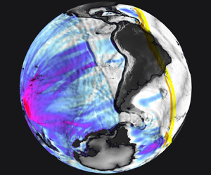
Figure 1. Equatorial views of the thermal atmospheric waves captured by five geostationary satellites on 15 January 2022. Time stamps are shown in coordinated universal time (UTC). Details about the measurements and estimate of the fluctuating temperature field ( $\mathcal {T}^\prime$) are given in Appendix A. The topography (colours) emphasises the main mountain ranges (values in the colourbar are in kilometres). The thermal wave is shown in grey scale clipped in the $\pm 0.1\ \mbox {K}$ range. Note that the $\mathcal {T}^\prime$ field was low-pass filtered with a cutoff length of $3\times 10^2\ \mbox {km}$ (see details in Appendix A). The thermal wave is seen to maintain a remarkable coherence from Tonga to its antipode despite travelling through weather systems, jet streams and mountain ranges. Whilst only the 9.6 $\mathrm {\mu }$m IR wavelength is shown here, similar patterns were found in all other IR spectral bands onboard the geostationary satellites, suggesting that the wave is coherent across the entire thickness of the troposphere. This thermal wave, triggered by the eruption, led to large-scale disturbances of the oceans’ surface and triggered tsunamis all around the world. The satellite data show the wave travelling back to Tonga in about 36 hrs and could capture at least three such cycles. The contours give the extracted wave position every hour from 05:00 to 19:00 UTC, and the blue dash line shows the wave position at the time shown in the snapshot.

Figure 2. Pressure fluctuations (in  $\mbox {hPa}$) measured from ground stations in mainland United States (NOAA ASOS data) and Japan (Weathernews Inc. Soratena network). The times shown are UTC times on 15 January 2022. The white contours give the location of the atmospheric thermal wave (see figure 1). Solid lines are on the hour, dash lines are 30 mins past the hour. The horizontal white bars provide an estimate for a distance of $10^3\ \mbox {km}$ (the map is shown on a longitude–latitude projection plane). The wavelength of the pressure wave approximately fits a 30-minute gap on the map, in agreement with the reported thermal wavelength of about $5\unicode{x2013}9 \times 10^2\ \mbox {km}$ (Matoza Reference Matoza2022; Wright et al. Reference Wright2022). The bottom panel gives a worldview of the significant waves listed by NOAA shortly after the thermal wave swept through. These wave heights contain runup values on the shores and should not be confused with sea-level displacements over oceanic basins for example (to be discussed later). The grey-scale map is lighten up as a function of water depth (brighter means deeper) and mountain ranges to give a general impression of the topography. The concentric lines give the extracted hourly thermal-wave position from 05:00 to 19:00 UTC on 15 January 2022. The west coast of the American continent and the East coast of Japan have experienced waves exceeding 1 m, despite being over 8000 km away from the volcano (upward triangle on the map). Remarkably, waves up to 50 cm high are reported in the Mediterranean sea, nearly on the antipode of the Tonga Islands (downward triangle on the map). These waves were observed hours earlier than those of a regular tsunami travelling from Tonga around the continents, and on amplitudes at least one order of magnitude higher than that expected for the energy released by the volcano near the Tonga Islands. They result from the energy transfer between the travelling thermal wave and the ocean that are not accounted for by regular tsunami warning systems.
Proudman was the first to theorize that water waves forced by a given atmospheric pressure distribution could be amplified under resonance (Proudman Reference Proudman1929). Since then, similar meteotsunami models have been proposed for weather systems/storms interacting with the ocean (see, e.g. Murty Reference Murty1984; Levin & Nosov Reference Levin and Nosov2009). These models correspond to the shallow-water equation (SWE) with a forcing that mimics the atmospheric pressure contributions, and are hereafter referred to as one-way coupled (OWC) as there is no feedback from the ocean to the atmosphere. Empiric velocities and spatial distributions, based on satellite data, ground pressure sensors and other observations, are used to construct an atmospheric pressure forcing  $p_a$ in the common OWC model,
 \begin{equation} \frac{{\rm D}}{{\rm D}t} \left[\begin{matrix} H \\ \boldsymbol{U} \end{matrix}\right] ={-} \left[\begin{matrix} H{\nabla}_{{\perp}} \boldsymbol{\cdot}\boldsymbol{U} \\ \rho_w^{{-}1}{\nabla}_{{\perp}} p_a+g{\nabla}_{{\perp}} \eta_1 \end{matrix}\right],\end{equation}
where  ${\rm D}/{\rm D} t$ is the material derivative, $H$ is the water depth, $\boldsymbol {U}$ is the depth-averaged in-plane (orthogonal to the vertical axis) velocity vector, ${\nabla }_{\perp }$ is the in-plane gradient operator, $\rho _w$ is the water density, $g$ is the gravitational acceleration and $\eta _1$ is the ocean's surface.
One-way coupled models have been used to study Rissaga storms in the Balearic sea (Monserrat, Ibbetson & Thorpe Reference Monserrat, Ibbetson and Thorpe1991; Renault et al. Reference Renault, Vizoso, Jansá, Wilkin and Tintoré2011; Romero, Vich & Ramis Reference Romero, Vich and Ramis2019), Abiki storms in Japan (Fukuzawa & Hibiya Reference Fukuzawa and Hibiya2020; Kubota et al. Reference Kubota, Saito, Chikasada and Sandanbata2021), storms in the Adriatic sea (Denamiel et al. Reference Denamiel, Šepić, Ivanković and Vilibić2019), storm resonance with tides (Williams et al. Reference Williams, Horsburgh, Schultz and Hughes2021), continental shelf resonance (Vennell Reference Vennell2007; Thiebaut & Vennell Reference Thiebaut and Vennell2011) and shore interactions (Chen & Niu Reference Chen and Niu2018; Dogan et al. Reference Dogan, Pelinovsky, Zaytsev, Metin, Ozyurt, Yalciner, Yalciner and Didenkulova2021). Following the Tonga event, OWC models were used to simulate the generated meteotsunami along one-dimensional great-circle lines starting from Tonga (Kakinuma Reference Kakinuma2022; Sekizawa & Kohyama Reference Sekizawa and Kohyama2022; Tanioka, Yamanaka & Nakagaki Reference Tanioka, Yamanaka and Nakagaki2022), two-dimensional (2-D) truncated regions of the globe (Heidarzadeh et al. Reference Heidarzadeh, Gusman, Ishibe, Sabeti and Šepić2022; Liu & Higuera Reference Liu and Higuera2022; Lynett et al. Reference Lynett2022; Pakoksung, Suppasri & Imamura Reference Pakoksung, Suppasri and Imamura2022; Peida & Xiping Reference Peida and Xiping2022; Ren, Higuera & Liu Reference Ren, Higuera and Liu2022; Yamada et al. Reference Yamada, Ho, Mori, Nishikawa and Yamamoto2022) and 2-D global simulations (Kubota, Saito & Nishida Reference Kubota, Saito and Nishida2022; Omira et al. Reference Omira, Ramalho, Kim, González, Kadri, Miranda, Carrilho and Baptista2022). In each of these cases, the atmospheric wave is stripped of its thermodynamic properties and acts as a rigid piston, assuming a sea-level forcing travelling at a set speed that is estimated from available observation data. For specific water depths, the OWC oceanic gravity-wave speed can match the imposed speed of the atmospheric pressure wave and produce a resonance that amplifies the water-surface displacement. This resonance is responsible for some of the wave heights reported in Kubota et al. (Reference Kubota, Saito and Nishida2022) and Omira et al. (Reference Omira, Ramalho, Kim, González, Kadri, Miranda, Carrilho and Baptista2022), and used as a key argument by these authors to explain the observed meteotsunamis in the Tonga event. However, since the amplification factor is a function of the set pressure-wave speed and the local water depth, the amplitude of induced water waves at a set depth can be directly modified by the choice of pressure-wave speed. This opens the door to numerical results that can be, to some extent, fitted to the observed data rather than reflect the ability of OWC models to predict the observed tsunami waves in events such as the Tonga one.
The thermal wave seen in figure 1 accompanied with the pressure disturbance observations seen in figure 2 are evidence of a thermodynamic process in the atmosphere. Isothermal and isobaric processes are not suitable to model the event given the observed in-phase thermal and pressure perturbations. The TEC perturbations in the ionosphere also indicate that density changes in the atmosphere are relevant to the process, supposedly ruling out an isochoric thermodynamic process. An isentropic process is then the most plausible constraint that would fit the observations and, therefore, the proposed coupled ocean-atmosphere dynamics consider that the perturbations in the atmosphere are isentropic in nature. This work presents a novel two-way coupled (TWC) model to study the propagation of long waves in the ocean-atmosphere system, where the atmosphere is modelled as an isentropic fully compressible layer capable of emulating the observations of the Tonga event. Other TWC models have been derived considering isothermal layers to study the air–sea waves after the Krakatoa eruption (Harkrider & Press Reference Harkrider and Press1967), considering steady atmospheric motion and heat exchange to model unstable air–sea interactions in the tropics (Philander, Yamagata & Pacanowski Reference Philander, Yamagata and Pacanowski1984), systems with multiple layers of incompressible fluids (Stewart & Dellar Reference Stewart and Dellar2010) and quasi-geostrophic ocean-atmosphere systems (Vallis Reference Vallis2017). Previous TWC models that consider compressible layers have used isothermal or steady motion to describe the atmosphere, these approaches are not suitable for this application. In this work, starting from first principles, two shallow layers are coupled through pressure and kinematic boundary conditions to model ocean-atmosphere interactions. The resulting TWC model represents the incompressible shallow-water ocean, the compressible shallow-layer atmosphere and the two-way coupling mechanisms between them.
The paper is structured as follows. Section 2 presents a detailed derivation of the governing equations for a general shallow layer of a compressible fluid. Section 3 describes the ocean and atmosphere layers, and the boundary conditions between them to obtain the TWC model. Section 4 shows the linear wave analysis and the resulting eigenmodes. Section 5 details the numerical results of the integration of the acoustic eigenmode as well as the direct simulation of the event, and their comparison with data from the Tonga event. Section 6 presents the discussion of the results and conclusions.
2. Shallow compressible-fluid equations
2.1. Non-dimensional compressible-fluid equations
Atmospheric observations following the Tonga event demonstrate that the pressure disturbances in the atmosphere can travel uninterrupted around the globe for several days (Matoza Reference Matoza2022), suggesting that dissipative effects may be neglected. From this observation the fluid is assumed to obey the non-dimensional compressible Euler equations (i.e. friction and heat losses are neglected),
 \begin{equation} St\frac{\partial}{\partial t} \left[\begin{matrix} \rho \\ \rho \boldsymbol{v} \\ \rho e_T \end{matrix}\right] + \boldsymbol{\nabla} \boldsymbol{\cdot} \left[\begin{matrix} \rho\boldsymbol{v} \\ \rho\boldsymbol{v}\otimes\boldsymbol{v} + Eu p {\boldsymbol{\mathsf{I}}}_3 \\ \rho\boldsymbol{v} e_T + Eu p\boldsymbol{v} \end{matrix}\right] = \left[\begin{matrix} 0 \\ \rho\boldsymbol{g}/Fr^2 \\ \rho\boldsymbol{v}\boldsymbol{\cdot}\boldsymbol{g}/Fr^2 \end{matrix}\right],\end{equation}
where  $\rho$, $\boldsymbol {v}$, $p$,
$p$,  $e_T$ are, respectively, the density, velocity vector, thermodynamic pressure and specific total energy of the fluid, with $e_T \equiv \boldsymbol {v}\boldsymbol {\cdot }\boldsymbol {v}/2 + e$, where $e$ is the specific internal energy of the fluid. Here $\boldsymbol {\nabla }\boldsymbol {\cdot }()$ is the divergence operator, $t$ is time and $\boldsymbol {v}\otimes \boldsymbol {v}$ is the velocity dyadic product. Non-dimensional numbers $St\equiv \ell _o /(t_o u_o)$, $Eu\equiv p_o/(\rho _o u_o^2)$, $Fr\equiv u_o/\sqrt {g_o\ell _o}$ are, respectively, the Strouhal, Euler and Froude numbers, where $t_o$, $u_o$, $\ell _o$, $p_o$, $\rho _o$, are reference time, speed, length, pressure, density, scales, respectively, and $g_o$ is a reference gravitational acceleration. Term $\boldsymbol {g}$ is the constant magnitude and direction gravitational acceleration vector non-dimensionalised by $g_o$ (tidal effects are neglected). Term ${\boldsymbol{\mathsf{I}}}_n$ is the identity tensor in $n$ dimensions. Without loss of generality, the reference time, pressure and speed are set to $t_o = \ell _o/u_o$, $p_o = \rho _o u_o^2$ and $u_o = \sqrt {g_o\ell _o}$, resulting in $St = Eu = Fr = 1$.
2.2. Depth averaging
Consider the geocentric spherical coordinate system with origin  $O$ at the centre of mass of the Earth, unitary basis $(O;(\boldsymbol {e}_{\mathcal {r}},\boldsymbol {e}_\theta,\boldsymbol {e}_\varphi ))$, coordinates $(\mathcal {r},\theta,\varphi )$ and position vector $\boldsymbol {r}=\mathcal {r}\boldsymbol {e}_\mathcal {r}$, where the radius $\mathcal {r}$ is defined as the distance from the origin, the colatitude $\theta$ is defined as the polar angle measured from the North Pole and the longitude $\varphi$ is defined as the angle in the equatorial plane measured from the prime meridian positive to the east. Integrating (2.1) in the radial direction $\boldsymbol {e}_\mathcal {r}$ between the two surfaces bounding a fluid layer results in the depth-averaged equations. Let $\mathscr {Z}_T(t,\mathcal {r},\theta,\varphi )=0$ and $\mathscr {Z}_B(t,\mathcal {r},\theta,\varphi )=0$ define, respectively, the top and bottom surfaces. Assuming these surfaces to be smooth (i.e. neglecting breaking waves and imposing $\partial \mathscr {Z}_i/\partial \mathcal {r}\neq 0$), the implicit function theorem states that these can be redefined as
 \begin{equation} \mathscr{Z}_i(t,\mathcal{r},\theta,\varphi)\equiv\eta_i(t,\theta,\varphi)-\mathcal{r}=0, \quad \text{with} \ i\in\{B,T\}. \end{equation}
The evolution of these surfaces represents the kinematic boundary condition given by
 \begin{equation} \frac{{\rm D}\mathscr{Z}_i}{{\rm D}t} =\frac{\partial\eta_i}{\partial t}+\boldsymbol{v}|_{\eta_i} \boldsymbol{\cdot}\nabla^{\eta_i}\mathscr{Z}_i=0, \end{equation}
where  $\boldsymbol {v}=[v_\mathcal {r},v_\theta,v_\varphi ]^{{\rm T}}$ is the velocity vector, the in-plane gradient operator for an arbitrary radius $a$ is defined as
 \begin{equation} \nabla^a\phi\equiv\left[\frac{\partial\phi}{\partial\mathcal{r}}, \frac{1}{a}\frac{\partial \phi}{\partial \theta}, \frac{1}{a\sin\theta}\frac{\partial \phi}{\partial \varphi}\right]^{{\rm T}}. \end{equation}
Throughout the text  $\phi$ and $\boldsymbol {f}$ denote an arbitrary scalar and vector field, respectively.
Let  $\langle \phi \rangle$ and $\bar {\phi }$ denote, respectively, the linear and logarithmic depth averages,
 \begin{equation} \langle \phi \rangle\equiv\frac{\displaystyle \int_{\eta_B}^{\eta_T}\phi \,\mathrm{d} \mathcal{r}}{\mathcal{H}} \quad\text{and}\quad \bar{\phi}\equiv\frac{\displaystyle \int_{z_B}^{z_T}\phi\,\mathrm{d} z}{\mathcal{L}},\end{equation}
where  $\mathcal {H}\equiv \eta _T-\eta _B$ is the non-dimensional layer thickness, $\mathcal {L}\equiv \ln (\eta _T/\eta _B)$ and $z=\ln (\mathcal {r})$, $z_B = \ln (\eta _B)$, $z_T = \ln (\eta _T)$.
Appendix B derives a general expression for the depth-averaged divergence of a vector field in spherical coordinates and its approximation under the thin-layer assumption. Using Leibniz integration rule and the results of Appendix B, the depth average of the time derivative and divergence are written as
 \begin{gather} \int_{\eta_B}^{\eta_T}\frac{\partial \phi}{\partial t}\, \mathrm{d} \mathcal{r} =\frac{\partial }{\partial t}(\mathcal{H}\langle \phi \rangle)- \left[\!\!\left[ {\phi\frac{\partial\eta}{\partial t}} \right]\!\!\right], \end{gather}
 \begin{gather}\int_{\eta_B}^{\eta_T}\boldsymbol{\nabla}\boldsymbol{\cdot}\boldsymbol{f}\,\mathrm{d} \mathcal{r}= {\nabla}_{{\perp}}^\mathcal{R} \boldsymbol{\cdot}(\mathcal{L}\mathcal{R}{\bar{\boldsymbol{f}}}_{{\perp}}) -[\![\,{\boldsymbol{f}\boldsymbol{\cdot}\nabla^\eta\mathscr{Z}} ]\!]+ 2\mathcal{L}\bar{\boldsymbol{f}}\boldsymbol{\cdot}\boldsymbol{e}_\mathcal{r}, \end{gather}
where  $\mathcal {R}$ is an arbitrary constant radius, the subscript $\perp$ denotes in-plane components of the vector (orthogonal to $\boldsymbol {e}_\mathcal {r}$), defined as ${\boldsymbol {f}}_{\perp }\equiv \mathcal {P}_\perp \boldsymbol {f}$ with $\boldsymbol {f}=[f_\mathcal {r},f_\theta,f_\varphi ]^{{\rm T}}$ and projection matrix $\mathcal {P}_\perp \equiv ( \begin {smallmatrix}0 & 1 & 0 \\ 0 & 0 & 1 \end {smallmatrix})$, and the double square brackets denote the difference between the top and bottom values evaluated on the inner sides of the bounding surfaces,
 \begin{equation} [\![ {\phi} ]\!]\equiv\phi|_{\eta_{T^-}}-\phi|_{\eta_{B^+}}, \quad \text{with } \phi|_{\eta_{T^-}}\equiv\lim_{\mathcal{r}\to\eta_{T^-}} \phi \quad \text{and} \quad \phi|_{\eta_{B^+}}\equiv\lim_{\mathcal{r}\to\eta_{B^+}} \phi, \end{equation}
and the in-plane divergence operator is
 \begin{equation} {\nabla}_{{\perp}}^\mathcal{R}\boldsymbol{\cdot}(\phi{\boldsymbol{f}}_{{\perp}}) =\frac{1}{\mathcal{R}\sin\theta}\left(\frac{\partial(\phi f_\theta\sin\theta)}{\partial\theta}+\frac{\partial(\phi f_\varphi)}{\partial\varphi}\right). \end{equation}
Using (2.3), (2.6) and (2.7), the depth average of the governing equations (2.1) is
 \begin{align} &\frac{\partial}{\partial t} \left[\begin{matrix} \mathcal{H} \langle \rho \rangle \\ \mathcal{H} \langle \rho v_\mathcal{r} \rangle \\ \mathcal{H} \langle \rho {\boldsymbol{v}}_{{\perp}} \rangle \\ \mathcal{H} \langle \rho e_{T} \rangle \end{matrix}\right] + {\nabla}_{{\perp}}^\mathcal{R} \boldsymbol{\cdot} \left[\begin{matrix} \mathcal{L}\mathcal{R} \overline{\rho{\boldsymbol{v}}_{{\perp}} } \\ \mathcal{L}\mathcal{R} \overline{\rho v_\mathcal{r}\,{\boldsymbol{v}}_{{\perp}} } \\ \mathcal{L}\mathcal{R}(\overline{\rho{\boldsymbol{v}}_{{\perp}} \otimes{\boldsymbol{v}}_{{\perp}} } + \bar{p}{\boldsymbol{\mathsf{I}}}_2) \\ \mathcal{L}\mathcal{R}(\overline{\rho e_{T}{\boldsymbol{v}}_{{\perp}} } + \overline{p{\boldsymbol{v}}_{{\perp}} }) \end{matrix}\right]\nonumber\\ &\quad = \left[\begin{matrix} 0 \\ -[\![ {p} ]\!]- \langle \rho \rangle g \mathcal{H} \\ [\![ {p{\nabla}_{{\perp}}^\eta\mathscr{Z}} ]\!] \\ [\![ {p\boldsymbol{v}\boldsymbol{\cdot}\nabla^\eta\mathscr{Z}} ]\!]- \langle \rho v_\mathcal{r} \rangle g\mathcal{H} \end{matrix}\right] -2\mathcal{L} \left[\begin{matrix} \overline{\rho v_\mathcal{r}} \\ \overline{\rho v_\mathcal{r} v_\mathcal{r}} \\ \overline{\rho v_\mathcal{r}{\boldsymbol{v}}_{{\perp}} } \\ \overline{\rho v_\mathcal{r} e_T}+\overline{p v_\mathcal{r}} \end{matrix}\right]{,} \end{align}
with  $g \equiv \boldsymbol {g}\boldsymbol {\cdot }\boldsymbol {e}_\mathcal {r}$ (note that $\boldsymbol {g}\boldsymbol {\cdot }\boldsymbol {e}_\theta = \boldsymbol {g}\boldsymbol {\cdot }\boldsymbol {e}_\varphi = 0$ from the assumptions).
2.3. Thin-layer assumption
Let  $d$ denote the characteristic length of the layer depth. Assuming the layer is thin compared with its radius ( $d\ll \mathcal {R}$), with $\mathcal {R}\equiv \mathcal {R}^*/\ell _o$, where $\mathcal {R}^*$ is the characteristic radius of the planet (for Earth $\mathcal {R}^*=6371\ \mbox {km}$). Defining $\delta \equiv d/\mathcal {R}$ and using the results of Appendix B.2 ( $\bar {\phi }=\langle \phi \rangle +\mathcal {O}(\delta ^2)$), (2.6) and (2.7) become
 \begin{gather} \int_{\eta_B}^{\eta_T}\frac{\partial \phi}{\partial t}\, \mathrm{d} \mathcal{r}=\frac{\partial }{\partial t}(\mathcal{H} \bar{\phi}) - \left[\!\!\left[ {\phi\frac{\partial\eta}{\partial t}} \right]\!\!\right]+\mathcal{O}(\delta^2), \end{gather}
 \begin{gather}\int_{\eta_B}^{\eta_T}\boldsymbol{\nabla}\boldsymbol{\cdot} \boldsymbol{f} \, \mathrm{d} \mathcal{r}= {\nabla}_{{\perp}}^\mathcal{R}\boldsymbol{\cdot}(\mathcal{H}{\bar{\boldsymbol{f}}}_{{\perp}}) +[\![ \,{\boldsymbol{f}\boldsymbol{\cdot}\boldsymbol{n}} ]\!]+ 2\frac{\mathcal{H}}{\eta_B}(\,\bar{\boldsymbol{f}}\boldsymbol{\cdot}\boldsymbol{e}_\mathcal{r}+ [\![ \, {{\boldsymbol{f}}_{{\perp}}\boldsymbol{\cdot}{\boldsymbol{n}}_{{\perp}}} ]\!]) +\mathcal{O}(\delta^2), \end{gather}
with the normal vector defined as  $\boldsymbol {n}_i\equiv -\nabla ^{\mathcal {R}}\mathscr {Z}_i$ and ${\boldsymbol {n}_i}_{\perp }={\mathcal {P}}_{\perp }\boldsymbol {n}_i$ (see Appendix B.2 for details).
Applying the above and using the surface evolution equation (2.3) on (2.10) results in the depth average thin-layer equations
 \begin{align} &\frac{\partial}{\partial t} \left[\begin{matrix} \mathcal{H} \bar{\rho} \\ \mathcal{H} \overline{\rho v_\mathcal{r}} \\ \mathcal{H} \overline{\rho {\boldsymbol{v}}_{{\perp}} } \\ \mathcal{H} \overline{\rho e_{T}} \end{matrix}\right] + {\nabla}_{{\perp}}^\mathcal{R} \boldsymbol {\cdot} \left[\begin{matrix} \mathcal{H} \overline{\rho{\boldsymbol{v}}_{{\perp}} } \\ \mathcal{H} \overline{\rho v_\mathcal{r}\,{\boldsymbol{v}}_{{\perp}} } \\ \mathcal{H} \overline{\rho{\boldsymbol{v}}_{{\perp}} \otimes{\boldsymbol{v}}_{{\perp}} }+ \mathcal{H} \bar{p}{\boldsymbol{\mathsf{I}}}_2 \\ \mathcal{H} \overline{\rho e_{T}{\boldsymbol{v}}_{{\perp}} }+ \mathcal{H} \overline{p{\boldsymbol{v}}_{{\perp}} } \end{matrix}\right]\nonumber\\ &\quad = \left[\begin{matrix} 0 \\ -[\![ {p} ]\!]- \bar{\rho}g \mathcal{H} \\ -[\![ {p{\boldsymbol{n}}_{{\perp}}} ]\!] \\ -[\![ {p\boldsymbol{v}\boldsymbol{\cdot}\boldsymbol{n}} ]\!]- \overline{\rho v_\mathcal{r}}g\mathcal{H} \end{matrix}\right] -2\frac{\mathcal{H}}{\eta_B} \left[\begin{matrix} \overline{\rho v_\mathcal{r}} \\ \overline{\rho v_\mathcal{r} v_\mathcal{r}} \\ \overline{\rho v_\mathcal{r}{\boldsymbol{v}}_{{\perp}} } + [\![ {p{\boldsymbol{n}}_{{\perp}}} ]\!]/2 \\ \overline{\rho v_\mathcal{r} e_T}+\overline{p v_\mathcal{r}}+[\![ {p{\boldsymbol{v}}_{{\perp}} \boldsymbol{\cdot}{\boldsymbol{n}}_{{\perp}}} ]\!]/2 \end{matrix}\right] + \mathcal{O}(\delta^2). \end{align}
2.4. Long-wave assumption
Considering a perturbation to the top surface  $\eta _T$ with a wavelength $L$ and amplitude $a$, the relative water depth is defined as $\varepsilon \equiv d/L$, where $d$ is the characteristic vertical length and $a\ll d$. Then, assuming long waves or shallow water ( $\varepsilon \ll 1$) the vertical velocity and the gradient of the surface become $\bar {v}_\mathcal {r}=\mathcal {O}(\varepsilon )$ and ${\nabla }_{\perp }^\mathcal {R}\eta =\mathcal {O}(a/L)$, and (2.13) becomes
 \begin{align} &\frac{\partial}{\partial t} \left[\begin{matrix} \mathcal{H} \bar{\rho} \\ \mathcal{H} \overline{\rho v_\mathcal{r}} \\ \mathcal{H} \overline{\rho {\boldsymbol{v}}_{{\perp}} } \\ \mathcal{H} \overline{\rho e_{T}} \end{matrix}\right] + {\nabla}_{{\perp}}^\mathcal{R} \boldsymbol{\cdot} \left[\begin{matrix} \mathcal{H} \overline{\rho{\boldsymbol{v}}_{{\perp}} } \\ \mathcal{H} \overline{\rho v_\mathcal{r} {\boldsymbol{v}}_{{\perp}} } \\ \mathcal{H} \overline{\rho{\boldsymbol{v}}_{{\perp}} \otimes{\boldsymbol{v}}_{{\perp}} } + \mathcal{H} \bar{p}{\boldsymbol{\mathsf{I}}}_2 \\ \mathcal{H} \overline{\rho e_{T}{\boldsymbol{v}}_{{\perp}} } + \mathcal{H} \overline{p{\boldsymbol{v}}_{{\perp}} } \end{matrix}\right]\nonumber\\ &\quad = \left[\begin{matrix} 0 \\ -[\![ {p} ]\!]- \bar{\rho}g\mathcal{H} \\ -[\![ {p{\boldsymbol{n}}_{{\perp}}} ]\!] \\ -[\![ {p\boldsymbol{v}\boldsymbol{\cdot}\boldsymbol{n}} ]\!] - \overline{\rho v_\mathcal{r}}g\mathcal{H} \end{matrix}\right] + \mathcal{O}(\delta\varepsilon), \end{align}
and the surface evolution equation (2.3) becomes
 \begin{equation} \frac{\partial\eta_i}{\partial t}-\boldsymbol{v}|_{\eta_i}\boldsymbol{\cdot}\boldsymbol{n}_i=\mathcal{O}(\delta\varepsilon).\end{equation}
2.5. Density-weighted average decomposition
Similarly to common practice in compressible-turbulence studies, density-weighted averages are recast following a Favre decomposition,  $\phi =\tilde {\phi }+\phi ''$, where $\tilde {\phi }=\overline {\rho \phi }/\bar {\rho }$. Here, the Reynolds decomposition uses the logarithmic depth average as $\phi =\bar {\phi }+\phi '$. With these decompositions, (2.14) becomes
 \begin{gather} \frac{\partial}{\partial t} \left[ \begin{matrix} \mathcal{H} \bar{\rho} \\ \mathcal{H} \bar{\rho}\tilde{v}_\mathcal{r} \\ \mathcal{H} \bar{\rho}{\tilde{\boldsymbol{v}}}_{{\perp}} \\ \mathcal{H} \bar{\rho}\tilde{e}_T \end{matrix} \right] \!+\! {\nabla}_{{\perp}}^\mathcal{R} \boldsymbol{\cdot} \left[ \begin{matrix} \mathcal{H} \bar{\rho}{\tilde{\boldsymbol{v}}}_{{\perp}} \\ \mathcal{H} \bar{\rho}\tilde{v}_\mathcal{r}{\tilde{\boldsymbol{v}}}_{{\perp}} \\ \mathcal{H} \bar{\rho}{\tilde{\boldsymbol{v}}}_{{\perp}}\otimes{\tilde{\boldsymbol{v}}}_{{\perp}} \!+\! \mathcal{H}\bar{p}{\boldsymbol{\mathsf{I}}}_2 \\ \mathcal{H} \bar{\rho}\tilde{e}_T{\tilde{\boldsymbol{v}}}_{{\perp}} + \mathcal{H} \bar{p}{\tilde{\boldsymbol{v}}}_{{\perp}} \end{matrix} \right] = \left[ \begin{matrix} 0 \\ -[\![ {p} ]\!]- \bar{\rho}g\mathcal{H} \\ -[\![ {p{\boldsymbol{n}}_{{\perp}}} ]\!] \\ -[\![ {p\boldsymbol{v}\boldsymbol{\cdot}\boldsymbol{n}} ]\!] - \bar{\rho}\tilde{v}_{\mathcal{r}} g\mathcal{H} \end{matrix} \right] + \mathcal{C} + \mathcal{O}(\delta\varepsilon),\end{gather}
where the in-plane velocity is decomposed as  ${\boldsymbol {v}}_{\perp } ={\tilde {\boldsymbol {v}}}_{\perp }+{\boldsymbol {v}}_{\perp }''$. The closure vector $\mathcal {C}$ corresponds to
 \begin{align} \mathcal{C}&={-}\partial \left[ \begin{matrix} 0, & 0, & 0, & \mathcal{H}\bar{\rho}\widetilde{{\boldsymbol{v}}_{{\perp}}^{''} \boldsymbol{\cdot}{\boldsymbol{v}}_{{\perp}}^{''}}/2 \end{matrix} \right]^{{\rm T}}/\partial t \nonumber\\ & \quad - {\nabla}_{{\perp}}^\mathcal{R} \boldsymbol {\cdot} \left[ \begin{matrix} 0, & \mathcal{H} \bar{\rho}\widetilde{v_\mathcal{r}^{\prime\prime}{\boldsymbol{v}}_{{\perp}}^{\prime\prime}}, & \mathcal{H} \bar{\rho}\widetilde{{\boldsymbol{v}}_{{\perp}}^{\prime\prime}\otimes{\boldsymbol{v}}_{{\perp}}^{\prime\prime}}, & \mathcal{H} \bar{\rho}\widetilde{ e_T^{\prime\prime}{\boldsymbol{v}}_{{\perp}}^{\prime\prime}}+ \mathcal{H} (\overline{p'{\boldsymbol{v}'}_{{\perp}}}+\bar{p}\overline{{\boldsymbol{v}}_{{\perp}}^{\prime\prime}}) \end{matrix} \right]^{{\rm T}}. \end{align}
Using Taylor series expansions, the closure vector  $\mathcal {C}$ is proven to be $\mathcal {O}(\delta \varepsilon )$ or, as shown in (B23), higher (see Appendix B.3 for details) and (2.16) becomes
 \begin{equation} \frac{\partial}{\partial t} \left[ \begin{matrix} \mathcal{H} \bar{\rho} \\ \mathcal{H} \bar{\rho}\tilde{v}_\mathcal{r} \\ \mathcal{H} \bar{\rho}{\tilde{\boldsymbol{v}}}_{{\perp}} \\ \mathcal{H} \bar{\rho}\tilde{e}_T \end{matrix} \right] + {\nabla}_{{\perp}}^\mathcal{R} \boldsymbol {\cdot} \left[ \begin{matrix} \mathcal{H} \bar{\rho}{\tilde{\boldsymbol{v}}}_{{\perp}} \\ \mathcal{H} \bar{\rho}\tilde{v}_\mathcal{r}{\tilde{\boldsymbol{v}}}_{{\perp}} \\ \mathcal{H} \bar{\rho}{\tilde{\boldsymbol{v}}}_{{\perp}}\otimes{\tilde{\boldsymbol{v}}}_{{\perp}} + \mathcal{H}\bar{p}{\boldsymbol{\mathsf{I}}}_2 \\ \mathcal{H} \bar{\rho}\tilde{e}_T{\tilde{\boldsymbol{v}}}_{{\perp}} + \mathcal{H} \bar{p}{\tilde{\boldsymbol{v}}}_{{\perp}} \end{matrix} \right] = \left[ \begin{matrix} 0 \\ -[\![ {p} ]\!]- \bar{\rho}g\mathcal{H} \\ -[\![ {p{\boldsymbol{n}}_{{\perp}}} ]\!] \\ -[\![ {p\boldsymbol{v}\boldsymbol{\cdot}\boldsymbol{n}} ]\!] - \bar{\rho}\tilde{v}_{\mathcal{r}} g\mathcal{H} \end{matrix} \right] + \mathcal{O}(\delta\varepsilon). \end{equation}
2.6. Long-wave expansion
The independent variables are rescaled based on the relative water depth  $\varepsilon$ as
 \begin{equation} t=\varepsilon^{{-}1}t^o,\quad {\boldsymbol{x}}_{{\perp}}=\varepsilon^{{-}1}{\boldsymbol{x}}_{{\perp}}^o,\quad \mathcal{r}=\mathcal{r}^o,\end{equation}
where the superscript  $^o$ denotes the rescaled quantities, and ${\boldsymbol {x}}_{\perp }$ is a position vector on the plane formed by the $\boldsymbol {e}_\theta$ and $\boldsymbol {e}_\varphi$ vectors. With this rescaling the variables become
 \begin{equation} \mathcal{H} = \mathcal{H}^o ,\quad \bar{\rho} = \bar{\rho}^o ,\quad \bar{p} = \bar{p}^o ,\quad \tilde{v}_\mathcal{r} = \varepsilon \tilde{v}_\mathcal{r}^o ,\quad {\tilde{\boldsymbol{v}}}_{{\perp}} = {\tilde{\boldsymbol{v}}}_{{\perp}}^o ,\quad \tilde{e}_T = \tilde{e}_T^o . \end{equation}
Analogous to standard practices in the derivation of the SWE (see, e.g. Narayanan Reference Narayanan2003), the coefficients of the rescaled variables are based on a set of modelling choices over the resulting equations. For the purposes of this work, these coefficients are derived based on the following constraints over the resulting leading-order equations and rescaled variables.
(i) The vertical momentum equation corresponds to the hydrostatic balance.
(ii) All the terms in the continuity equation are of the same order.
(iii) All the terms in the in-plane momentum equation are of the same order.
(iv) Pressure and density changes follow the same scaling (i.e. they are related via the isentropic constraint).
Constraints (i)–(iii) are used to recover the SWE in the incompressible-flow case and constraint (iv) is added for compatibility with the internal-energy equation in the compressible-flow case. Note that the resulting leading-order equations will differ for another set of considerations. Appendix B.4 describes the derivation of the coefficients and the leading-order equations. From here on, the superscript  $^o$ is omitted for readability, and the resulting leading-order equations are
 \begin{align} \frac{\partial}{\partial t} \left[ \begin{matrix} \mathcal{H} \bar{\rho} \\ 0 \\ \mathcal{H} \bar{\rho}{\tilde{\boldsymbol{v}}}_{{\perp}} \\ \mathcal{H} \bar{\rho}\tilde{e}_T \end{matrix} \right] +{\nabla}_{{\perp}}^{\mathcal{R}} \boldsymbol{\cdot} \left[ \begin{matrix} \mathcal{H} \bar{\rho}{\tilde{\boldsymbol{v}}}_{{\perp}} \\ 0 \\ \mathcal{H} \bar{\rho}{\tilde{\boldsymbol{v}}}_{{\perp}}\otimes{\tilde{\boldsymbol{v}}}_{{\perp}} + \mathcal{H}\bar{p}{\boldsymbol{\mathsf{I}}}_2 \\ \mathcal{H} \bar{\rho}\tilde{e}_T{\tilde{\boldsymbol{v}}}_{{\perp}} + \mathcal{H} \bar{p}{\tilde{\boldsymbol{v}}}_{{\perp}} \end{matrix} \right] = \left[ \begin{matrix} 0 \\ -[\![ {p} ]\!]- \bar{\rho}g\mathcal{H} \\ -[\![ {p{\boldsymbol{n}}_{{\perp}}} ]\!] \\ -[\![ {p\boldsymbol{v}\boldsymbol{\cdot}\boldsymbol{n}} ]\!] - \bar{\rho}\tilde{v}_{\mathcal{r}} g\mathcal{H} \end{matrix} \right] + \mathcal{O}(\delta\varepsilon), \end{align}
and
 \begin{equation} \frac{\partial\eta_i}{\partial t}-\boldsymbol{v}|_{\eta_i}\boldsymbol{\cdot}\boldsymbol{n}_i=\mathcal{O}(\delta\varepsilon). \end{equation}
2.7. Isentropic-flow constraint
The kinetic energy equation is obtained by taking the dot product of the Favre average velocity  $\tilde {\boldsymbol {v}}$ with the momentum-balance statement in (2.21), including the radial components. Subtracting the result from the total energy equation in (2.21) yields the governing equation for the Favre-averaged internal energy after application of the continuity equation ${\nabla }_{\perp }^\mathcal {R}\boldsymbol {\cdot }{\tilde {\boldsymbol {v}}}_{\perp }= -(\mathcal {H}\bar {\rho })^{-1}{\rm D}(\mathcal {H}\bar {\rho })/{\rm D}t$, i.e.
 \begin{equation} \mathcal{H}\bar{\rho}\frac{{\rm D} \tilde{e}}{{\rm D} t} -\frac{\bar{p}}{\bar{\rho}}\frac{{\rm D} (\mathcal{H}\bar{\rho})}{{\rm D} t} +[\![ {p\boldsymbol{v}''\boldsymbol{\cdot}\boldsymbol{n}} ]\!]=\mathcal{O}(\delta\varepsilon).\end{equation}
 Rearranging the material derivative of  $\mathcal {H}\bar {\rho }$, introducing $p = \bar {p} + p'$, noting that $[\![ {\bar {p}\boldsymbol {f}} ]\!] = \bar {p}[\![ {\boldsymbol {f}} ]\!]$ and $[\![ {p'\boldsymbol {v}''\boldsymbol {\cdot }\boldsymbol {n}} ]\!]=\mathcal {O}(\delta \varepsilon )$ (see Appendix B.3 for details) gives
 \begin{equation} \mathcal{H}\bar{\rho}\frac{{\rm D} \tilde{e}}{{\rm D}t}={-}\mathcal{H}\bar{\rho}\,\bar{p}\frac{{\rm D}}{{\rm D}t}\left(\frac{1}{\bar{\rho}}\right) + \bar{p}\left( \frac{{\rm D} \mathcal{H}}{{\rm D}t} - [\![ {\boldsymbol{v}''\boldsymbol{\cdot}\boldsymbol{n}} ]\!]\right) + \mathcal{O}(\delta\varepsilon). \end{equation}
Applying (2.22) at  $\eta _T$ and $\eta _B$, introducing the Favre decomposition ${\boldsymbol {v}}_{\perp } = {\tilde {\boldsymbol {v}}}_{\perp } + {\boldsymbol {v}}_{\perp }''$ and $v_\mathcal {r} = \tilde {v}_\mathcal {r} + v_\mathcal {r}''$, and subtracting the results yields $D\mathcal {H}/Dt = [\![ {v_\mathcal {r}''} ]\!] + \mathcal {O}(\delta \varepsilon )$. The internal-energy equation becomes
 \begin{equation} \mathcal{H}\bar{\rho}\frac{{\rm D} \tilde{e}}{{\rm D}t}={-}\mathcal{H}\bar{\rho}\,\bar{p}\frac{{\rm D}}{{\rm D}t}\left(\frac{1}{\bar{\rho}}\right) + \bar{p}[\![ {\boldsymbol{v}''\boldsymbol{\cdot}(\boldsymbol{e}_\mathcal{r}-\boldsymbol{n})} ]\!] + \mathcal{O}(\delta\varepsilon). \end{equation}
The long-wave assumption implies that  $\boldsymbol {n} = \boldsymbol {e}_\mathcal {r} + \mathcal {O}(\varepsilon )$. The thin-layer assumption implies that $\boldsymbol {v}'' = \mathcal {O}(\delta )$. Hence, $\boldsymbol {v}''\boldsymbol {\cdot }(\boldsymbol {e}_\mathcal {r}-\boldsymbol {n}) = \mathcal {O}(\delta \varepsilon$), and the internal-energy equation reduces to
 \begin{equation} \mathcal{H}\bar{\rho}\left[\frac{{\rm D} \tilde{e}}{{\rm D}t}+\bar{p}\frac{{\rm D}}{{\rm D}t}\left(\frac{1}{\,\bar{\rho}\,}\right)\right] = \mathcal{O}(\delta\varepsilon). \end{equation}
Equation (2.26) implies that, to first order in  $\delta \varepsilon$, the entropy of a material element of a thin layer is conserved along its trajectory in space–time. The flow is therefore isentropic.
Let  $\mathcal {V}\equiv 1/\bar {\rho }$ be the specific volume of the layer (not necessarily the depth average value of $\rho ^{-1}$). Let $\mathcal {S}$ be the specific entropy of the layer (not necessarily the Favre-averaged value of the specific entropy). Considering that $\tilde {e}$ depends on the state variables $\mathcal {V}$ and $\mathcal {S}$ (having previously ignored any chemical-potential dependency), the total differential of $\tilde {e}$ is
 \begin{equation} \mathrm{d}\tilde{e}=\left(\frac{\partial\tilde{e}}{\partial \mathcal{V}}\right)_{\mathcal{S}}\, \mathrm{d}\mathcal{V}+\left(\frac{\partial\tilde{e}}{\partial\mathcal{S}} \right)_{\mathcal{V}}\, \mathrm{d}\mathcal{S}. \end{equation}
Assuming that any material element of the layer evolves under the isentropic constraint  $\mathrm {d}\mathcal {S}=0$, (2.26) and (2.27) give
 \begin{equation} \bar{p} ={-} \left(\frac{\partial\tilde{e}}{\partial \mathcal{V}}\right)_{\mathcal{S}}. \end{equation}
Since the thermodynamic pressure  $\bar {p}$ depends on the state variables $\mathcal {V}$ and $\mathcal {S}$, the isentropic constraint imposes that
 \begin{equation} \mathrm{d}\bar{p}=\left(\frac{\partial\bar{p}}{\partial \mathcal{V}} \right)_{\mathcal{S}}\, \mathrm{d}\mathcal{V} = \left(\frac{\partial\bar{p}}{\partial \bar{\rho}}\right)_{\mathcal{S}}\, \mathrm{d}\bar{\rho} = \mathscr{C}^2\, \mathrm{d}\bar{\rho}, \end{equation}
where  $\mathscr {C} \equiv [(\partial \bar {p}/\partial \bar {\rho })_{\mathcal {S}}]^{1/2}$ is the isentropic sound speed of the layer.
The total energy equation in (2.21) can thus be replaced by
 \begin{equation} \frac{{\rm D} \bar{p}}{{\rm D} t} = \mathscr{C}^2 \frac{{\rm D} \bar{\rho}}{{\rm D} t}, \end{equation}
where  $\mathscr {C}$ is evaluated from the depth-averaged variables.
3. Two-way coupled ocean-atmosphere model
The compressible shallow-layer equation derived in the previous section is now applied to form a coupled ocean-atmosphere system. Figure 3 illustrates the configuration along with some key notations. For clarity, the following notation is used to describe each layer
 \begin{align} &\text{Ocean}: \qquad\qquad H\equiv\eta_1-\eta_0,\quad\quad \boldsymbol{U}\equiv{\tilde{\boldsymbol{v}}}_{{\perp}},\quad\quad\rho_w\equiv\bar{\rho},& \end{align}
 \begin{align} &\text{Atmosphere}:\qquad h\equiv\eta_2-\eta_1,\quad\quad\ \boldsymbol{u}\equiv{\tilde{\boldsymbol{v}}}_{{\perp}},\quad\quad\ \ \varrho\equiv\bar{\rho},\quad\quad\ {\rm \pi}\equiv\bar{p}. \end{align}
The coupled system is bounded by the seabed,  $\eta _0$, at its bottom, and the ‘top’ of the atmosphere, $\eta _2$, on the outer-space side. The ocean-atmosphere interface is denoted by $\eta _1$. All variables correspond to the leading order terms of the long-wave and thin-layer expansion. With these definitions, the material derivative for each layer is denoted by:
 \begin{equation} \frac{{\rm D} ^{\boldsymbol{U}}()}{{\rm D}t}\equiv\frac{\partial()}{\partial t}+\boldsymbol{U}\boldsymbol{\cdot}{\nabla}_{{\perp}}^\mathcal{R}()\quad \text{and}\quad \frac{{\rm D} ^{\boldsymbol{u}}()}{{\rm D}t}\equiv\frac{\partial()}{\partial t}+\boldsymbol{u}\boldsymbol{\cdot}{\nabla}_{{\perp}}^\mathcal{R}(). \end{equation}
Figure 3. Sketch of the ocean-atmosphere configuration and main notations used. The ocean is shown in blue and the atmosphere in ivory. Note that the characteristic thickness of a layer,  $d$, is used interchangeably between the ocean and the atmosphere. The model assumes that both the thin-layer ( $\mathcal {R}\gg d$) and long-wave ( $L\gg d$) assumptions apply.
3.1. Shallow ocean equations
The seawater density,  $\rho _w$, is assumed constant and uniform. The continuity equation in (2.21) simplifies to ${\rm D}^{\boldsymbol {U}} H/{\rm D} t = - H {\nabla }_{\perp }^\mathcal {R}\boldsymbol {\cdot }\boldsymbol {U}$. The radial component of the momentum equation in (2.21) becomes $[\![ {p} ]\!] = p|_{\eta _1} - p|_{\eta _0} = -\rho _wg H$. This is the hydrostatic balance (‘ $\mathrm {d} p = - \rho _wg\,\mathrm {d} \mathcal {r}$’), which, in the uniform-density case integrates to the linear profile $p(\mathcal {r}) = p|_{\eta _1} - \rho _wg(\mathcal {r}-\eta _1)$. Depth averaging gives $\bar {p}=p|_{\eta _1} + \rho _wg H/2 +\mathcal {O}(\delta ^2)$. Substituting these in (2.21) yields
 \begin{equation} \frac{{\rm D}^{\boldsymbol{U}}}{{\rm D} t} \left[\begin{matrix} H \\ \boldsymbol{U} \end{matrix}\right] ={-}\left[\begin{matrix} H {\nabla}_{{\perp}}^\mathcal{R}\boldsymbol{\cdot}\boldsymbol{U} \\ \rho_w^{{-}1}{\nabla}_{{\perp}}^\mathcal{R} p|_{\eta_1} + g{\nabla}_{{\perp}}^\mathcal{R}\eta_1 \end{matrix}\right].\end{equation}
Note that the internal-energy equation is removed from the ocean-layer dynamics since ‘pressure’ in the uniform-density (and isothermal) framework purely assumes a kinematic role and not a thermodynamic one. Retaining the internal-energy equation would over-constrain the dynamical system.
Equation (3.4) is strictly the same dynamical equation as that of the OWC models (see (1.1)). However, note that the TWC model will let  $\eta _1$, $\boldsymbol {U}$ and $p|_{\eta _1}$ all be influenced by the atmospheric layer, whereas OWC models prescribe assumed space–time dependencies for $p|_{\eta _1}$ that do not depend on the evolution of the system. In the absence of a pressure gradient on the ocean surface and a fixed seabed position, (3.4) is in a closed form and is strictly equivalent to the classical SWE (see, e.g. Vallis Reference Vallis2017), referred here to as the zero-way coupling (ZWC) model.
3.2. Shallow atmosphere equations
The continuity and in-plane momentum equations in (2.21) are rearranged in primitive form and the total energy equation replaced by (2.30) to give
 \begin{equation} \frac{{\rm D} ^{\boldsymbol{u}}}{{\rm D} t} \left[\begin{matrix} \varrho \\ \boldsymbol{u} \\ {\rm \pi}\end{matrix}\right] ={-}\left[\begin{matrix} \varrho\varPsi \\ (\varrho h)^{{-}1}({\nabla}_{{\perp}}^\mathcal{R}(h{\rm \pi})-p|_{\eta_1} {\nabla}_{{\perp}}^\mathcal{R} h) -g{\nabla}_{{\perp}}^\mathcal{R}\eta_2 \\ \varrho\varPsi\mathscr{C}^2 \end{matrix}\right],\end{equation}
where  $\varPsi \equiv h^{-1}[{\nabla }_{\perp }^\mathcal {R}\boldsymbol {\cdot }(h\boldsymbol {u})+\partial h/\partial t]$ and $p|_{\eta _1} = p|_{\eta _2} + \varrho g h$.
Air is assumed to be thermally ( $p^* = \rho ^* \mathscr {R}_{air} T^*$) and calorically ( $\mathrm {d}e^* = c_v \, \mathrm {d}T^*$) perfect (humidity and phase changes are not taken into account), where the gas constant $\mathscr {R}_{air}$ and the specific heat at constant volume $c_v$ are true dimensional constants. Further assuming $e^*(T^*=0)=0$ results in $e^*=c_v T^*$. Using the reference pressure $p_o = \rho _o u_o^2$ and defining the non-dimensional temperature as $T \equiv \mathscr {R}_{air} T^*/u_o^2$, the thermal equation of state (EoS) becomes $p=\rho T$ and the caloric EoS becomes $e = (c_v/\mathscr {R}_{air}) T$. Depth-averaging both gives $\bar {p} = \bar {\rho }\tilde {T}$ and $\tilde {e} = (c_v/\mathscr {R}_{air}) \tilde {T}$, and injecting these in (2.27) using (2.28) yields
 \begin{equation} \mathrm{d}\bar{p}=\gamma\frac{\bar{p}}{\bar{\rho}}\, \mathrm{d}\bar{\rho} +\bar{\rho}\frac{\mathscr{R}_{air}}{c_v} \left(\frac{\partial\tilde{e}}{\partial\mathcal{S}}\right)_{\mathcal{V}}\, \mathrm{d}\mathcal{S}, \end{equation}
where  $\gamma \equiv c_p/c_v$, $c_p$ is the specific heat at constant pressure, and $\mathscr {R}_{air} = c_p-c_v$ (Mayer's relation). Thus, using (2.29), the isentropic sound speed of the layer is
 \begin{equation} \mathscr{C} = \sqrt{\gamma \frac{\bar{p}}{\bar{\rho}}} = \sqrt{\gamma \frac{\rm \pi}{\varrho}}, \end{equation}
where  ${\rm \pi}$ and $\varrho$ are, respectively, the (logarithmic) depth-averaged pressure and density. Section 5 will show that in standard atmospheric conditions this speed, evaluated on the entire thickness of the troposphere (and beyond), matches that of the so-called Lamb wave invoked in OWC models.
3.3. Boundary conditions
3.3.1. Edge boundary conditions
The seabed ( $\eta _0$) is non-uniform but stationary. The outer-space boundary ( $\eta _2$) is assumed uniform and stationary. The steady edge boundary conditions therefore impose that $H + h = \eta _2-\eta _0$ remains constant with time,
 \begin{equation} \frac{\partial H}{\partial t}+\frac{\partial h}{\partial t}=0.\end{equation}
The rather strict constraints on  $\eta _2$ can be relaxed in future studies by adding further atmospheric layer(s) to better account for the high-atmosphere physics (Aa et al. Reference Aa, Zhang, Erickson, Vierinen, Coster, Goncharenko, Spicher and Rideout2022), which is beyond the scope of this study, where $\eta _2$ is placed at the interface with the ionosphere, which is modelled as a uniform semi-infinite vacuum (i.e. Earth is placed in a vacuum from the ionosphere outwards).
3.3.2. Interface conditions
The surface evolution equation (2.22) is evaluated on the upper ( $+$) and lower ( $-$) sides of the $i^\mathrm {th}$ layer,
 \begin{equation} \frac{\partial\eta_i^{{\pm}}}{\partial t} = \boldsymbol{v}|_{\eta_i^{{\pm}}}\boldsymbol{\cdot}\boldsymbol{n}_i^{{\pm}}+\mathcal{O}(\delta\varepsilon). \end{equation}
It follows that two neighbouring layers remain in contact if  $\eta _i^+ = \eta _i^{-}$ at all times, i.e. if $\boldsymbol {v}|_{\eta _i^+}\boldsymbol {\cdot }\boldsymbol {n}_i^+ = \boldsymbol {v}|_{\eta _i^-}\boldsymbol {\cdot }\boldsymbol {n}_i^-$. Since $\boldsymbol {v}$ (the local velocity field) is continuous, the surface evolution equation enforces that no layer detaches from its neighbour. The ocean and atmosphere are thus in contact at all times by simply requiring that they initially satisfy $\eta _1^+(t=0) = \eta _1^-(t=0) = \eta _1(t=0)$. Note, however, that depth-averaged velocities are not required (nor expected) to be continuous across the interface (e.g. the depth-averaged velocity of the atmosphere will generally not be equal to that of the ocean).
3.3.3. Pressure boundary conditions
Pressure is considered continuous across the ocean-atmosphere interface (e.g. surface tension is negligible on long waves). On the outer-space side, pressure is assumed to be zero given the vacuum assumption i.e.  $p|_{\eta _2}=0$. The jump condition (from the radial component of the governing equation) across the atmospheric layer simplifies to
 \begin{equation} p|_{\eta_1} = \varrho g h.\end{equation}
3.4. Two-way coupled equations
Combining (3.8) with the water-layer continuity equation (3.4) yields
 \begin{equation} \frac{\partial h}{\partial t}= {\nabla}_{{\perp}}^\mathcal{R}\boldsymbol{\cdot}(H \boldsymbol{U}). \end{equation}
Moreover, boundary conditions  $p|_{\eta _2} = 0$ and ${\nabla }_{\perp }^\mathcal {R}\eta _2 = \boldsymbol {0}$ reduce the atmosphere-layer equation to
 \begin{equation} \frac{{\rm D} ^{\boldsymbol{u}}}{{\rm D} t} \left[\begin{matrix} \varrho \\ \boldsymbol{u} \\ {\rm \pi}\end{matrix}\right] ={-}\left[\begin{matrix} \varrho\varPsi \\ (\varrho h)^{{-}1}{\nabla}_{{\perp}}^\mathcal{R}(h{\rm \pi}) +g{\nabla}_{{\perp}}^\mathcal{R}\eta_1\\ \varrho\varPsi\mathscr{C}^2 \end{matrix}\right],\end{equation}
with  $\varPsi = h^{-1}{\nabla }_{\perp }^\mathcal {R}\boldsymbol {\cdot }(h\boldsymbol {u}+H\boldsymbol {U})$.
Equations (3.4) and (3.12) can be solved simultaneously to form the TWC model
 \begin{equation}
\frac{\partial}{\partial t} \left[\begin{matrix} \eta_1 \\
\boldsymbol{U} \\ \varrho \\ \boldsymbol{u} \\ {\rm \pi}
\end{matrix}\right] + \left[\begin{matrix}
\boldsymbol{U}\boldsymbol{\cdot}{\nabla}_{{\perp}}^\mathcal{R}
H \\
(\boldsymbol{U}\boldsymbol{\cdot}{\nabla}_{{\perp}}^\mathcal{R})\boldsymbol{U}
\\
\boldsymbol{u}\boldsymbol{\cdot}{\nabla}_{{\perp}}^\mathcal{R}
\varrho \\
(\boldsymbol{u}\boldsymbol{\cdot}{\nabla}_{{\perp}}^\mathcal{R})\boldsymbol{u}
\\
\boldsymbol{u}\boldsymbol{\cdot}{\nabla}_{{\perp}}^\mathcal{R}
{\rm \pi} \end{matrix}\right] ={-}\left[\begin{matrix}
H{\nabla}_{{\perp}}^\mathcal{R}\boldsymbol{\cdot}\boldsymbol{U}
\\ \rho_w^{{-}1}{\nabla}_{{\perp}}^\mathcal{R}(\varrho g h)
+ g{\nabla}_{{\perp}}^\mathcal{R}\eta_1 \\ \varrho\varPsi
\\ (\varrho h)^{{-}1}{\nabla}_{{\perp}}^\mathcal{R}(h{\rm \pi})
+g{\nabla}_{{\perp}}^\mathcal{R}\eta_1 \\ \varrho\varPsi\mathscr{C}^2
\end{matrix}\right],\end{equation}
\begin{equation}
\frac{\partial}{\partial t} \left[\begin{matrix} \eta_1 \\
\boldsymbol{U} \\ \varrho \\ \boldsymbol{u} \\ {\rm \pi}
\end{matrix}\right] + \left[\begin{matrix}
\boldsymbol{U}\boldsymbol{\cdot}{\nabla}_{{\perp}}^\mathcal{R}
H \\
(\boldsymbol{U}\boldsymbol{\cdot}{\nabla}_{{\perp}}^\mathcal{R})\boldsymbol{U}
\\
\boldsymbol{u}\boldsymbol{\cdot}{\nabla}_{{\perp}}^\mathcal{R}
\varrho \\
(\boldsymbol{u}\boldsymbol{\cdot}{\nabla}_{{\perp}}^\mathcal{R})\boldsymbol{u}
\\
\boldsymbol{u}\boldsymbol{\cdot}{\nabla}_{{\perp}}^\mathcal{R}
{\rm \pi} \end{matrix}\right] ={-}\left[\begin{matrix}
H{\nabla}_{{\perp}}^\mathcal{R}\boldsymbol{\cdot}\boldsymbol{U}
\\ \rho_w^{{-}1}{\nabla}_{{\perp}}^\mathcal{R}(\varrho g h)
+ g{\nabla}_{{\perp}}^\mathcal{R}\eta_1 \\ \varrho\varPsi
\\ (\varrho h)^{{-}1}{\nabla}_{{\perp}}^\mathcal{R}(h{\rm \pi})
+g{\nabla}_{{\perp}}^\mathcal{R}\eta_1 \\ \varrho\varPsi\mathscr{C}^2
\end{matrix}\right],\end{equation}
with  $h = \eta _2-\eta _1$, $H = \eta _1-\eta _0$, $\varPsi = h^{-1}{\nabla }_{\perp }^\mathcal {R}\boldsymbol {\cdot }(h\boldsymbol {u}+H\boldsymbol {U})$, $\mathscr {C}^2 = \gamma {\rm \pi}/\varrho$, where $\gamma$ is a constant (set to $1.4$). Note that $\eta _0$ and $\eta _2$ are set initially and do not change, hence, the choice to integrate $\eta _1$ rather than $H$ and $h$ that can be evaluated directly from $\eta _1$ and the initial $\eta _0$ and $\eta _2$ profiles.
4. Eigenmodes
4.1. Quasi-linear one-dimensional form
The one-dimensional quasi-linear form is found by projecting (3.13) along a great circle with coordinate  $s$ along which $\boldsymbol {e}_{s}$ is the unit vector tangent to the sphere of radius $\mathcal {R}$. Letting $\boldsymbol {\mu } \equiv [\eta _1,U,\varrho,u,{\rm \pi} ]^{{\rm T}}$ denote the vector of primitive variables, with $U=\boldsymbol {U}\boldsymbol {\cdot }\boldsymbol {e}_{s}$ and $u=\boldsymbol {u}\boldsymbol {\cdot }\boldsymbol {e}_{s}$, the projected equation is
 \begin{equation} \frac{\partial\boldsymbol{\mu}}{\partial t} + {\boldsymbol{\mathsf{A}}} \frac{\partial\boldsymbol{\mu}}{\partial s} =\boldsymbol{0}, \quad\text{with } {\boldsymbol{\mathsf{A}}}\equiv \left[ \begin{matrix} U & H & 0 & 0 & 0 \\ g(1-\beta) & U & \dfrac{g h}{\rho_w} & 0 & 0 \\ 0 & \varrho\chi & u & \varrho & 0 \\ g-\dfrac{\rm \pi}{\varrho h} & 0 & 0 & u & \dfrac{1}{\varrho}\\ 0 & \varrho\chi\mathscr{C}^2 & 0 & \varrho\mathscr{C}^2 & u \end{matrix} \right],\end{equation}
where  $\beta \equiv \varrho /\rho _w$ and $\chi \equiv H/h$ are, respectively, the air–water density ratio and ocean-atmosphere depth ratio.
4.2. Linear waves
Let  $\boldsymbol {\mu }_0 \equiv [(\eta _1)_0,U_0,\varrho _0,u_0,{\rm \pi} _0]^{{\rm T}}$ denote a stationary solution to the quasi-linear equation (4.1), and $\boldsymbol {\mu }_1 \equiv [(\eta _1)_1,U_1,\varrho _1,u_1,{\rm \pi} _1]^{{\rm T}}$ be a perturbation around the stationary solution, such that $\boldsymbol {\mu } = \boldsymbol {\mu }_0 + \boldsymbol {\mu }'$, where $\boldsymbol {\mu }'\equiv \zeta \boldsymbol {\mu }_1$ denotes the scaled perturbations and $\zeta$ is a smallness parameter ( $\zeta \ll 1$). Replacing $\boldsymbol {\mu } = \boldsymbol {\mu }_0 + \zeta \boldsymbol {\mu }_1$ in (4.1) and collecting terms based on their $\zeta$ order results in
 \begin{align} \zeta^0:\qquad\qquad\qquad\qquad\qquad\ \qquad\qquad\qquad\qquad\qquad {\boldsymbol{\mathsf{A}}}_0\frac{\partial\boldsymbol{\mu}_0}{\partial s} &=\boldsymbol{0},\end{align}
 \begin{align} \zeta^1:\qquad\qquad\qquad\qquad\qquad\qquad\quad\frac{\partial\boldsymbol{\mu}_1}{\partial t}+{\boldsymbol{\mathsf{A}}}_1\frac{\partial\boldsymbol{\mu}_0}{\partial s}+{\boldsymbol{\mathsf{A}}}_0\frac{\partial\boldsymbol{\mu}_1}{\partial s} &=\boldsymbol{0}, \end{align}
where  ${\boldsymbol{\mathsf{A}}}_0$ and ${\boldsymbol{\mathsf{A}}}_1$ indicate that ${\boldsymbol{\mathsf{A}}}$ is evaluated using $\boldsymbol {\mu }_0$ and $\boldsymbol {\mu }_1$, respectively. Assuming a uniform base flow, i.e. $\partial \boldsymbol {\mu }_0/\partial s = \boldsymbol {0}$, (4.2) is satisfied and (4.3) simplifies to
 \begin{equation} \frac{\partial\boldsymbol{\mu}_1}{\partial t}+{\boldsymbol{\mathsf{A}}}_0\frac{\partial\boldsymbol{\mu}_1}{\partial s}=\boldsymbol{0}. \end{equation}
Plane-wave solutions to (4.4) are sought in the form  $\boldsymbol {\mu }_1=\hat {\boldsymbol {\mu }} \exp [\mathrm {i}(\omega t-ks)]$, where $k\in \mathbb {R}_{>0}$ is the wavenumber, $\omega \in \mathbb {R}_{>0}$ is the angular frequency, $\mathrm {i}^2=-1$, and $\hat {\boldsymbol {\mu }}=[\hat {\eta }_1,\hat {U},\hat {\varrho },\hat {u},\hat {{\rm \pi} }]^{{\rm T}}$ is a vector of eigenfunctions for the primitive variables. Substituting $\boldsymbol {\mu }_1$ using the eigenfunctions in (4.4) yields
 \begin{equation} ({\boldsymbol{\mathsf{A}}}_0 - \lambda{\boldsymbol{\mathsf{I}}}_5)\hat{\boldsymbol{\mu}} = \boldsymbol{0}, \end{equation}
with  $\lambda \equiv \omega /k$. Non-trivial solutions to (4.5) exist if
 \begin{equation} \det{({\boldsymbol{\mathsf{A}}}_0 - \lambda{\boldsymbol{\mathsf{I}}}_5)}= \lambda (-\lambda^4 + (\mathscr{C}_w+\mathscr{C}_0^2)\lambda^2 + \mathscr{C}_w[\mathscr{C}_0^2({\beta_0}-1)+{\beta_0} \mathscr{C}_a - \mathscr{C}_T])=0, \end{equation}
where quiescent base flows for air ( $U_0=0$) and water ( $u_0=0$) have been assumed, $\mathscr {C}_w\equiv \sqrt {g H_0}$ and $\mathscr {C}_a\equiv \sqrt {g h_0}$ are the base flow gravity-wave speeds in the ocean and atmosphere layers, respectively, and $\mathscr {C}_0 \equiv \sqrt {\gamma {\rm \pi}_0/\varrho _0}$ and $\mathscr {C}_T\equiv \sqrt {{\rm \pi} _0/\varrho _0}$ are the base flow sound speed and Newton's sound speed in the atmospheric layer and $\beta _0 = \varrho _0/\rho _w$. The roots of (4.6) are
 \begin{equation} \lambda=0\quad \text{and} \quad \lambda^2 = \tfrac{1}{2} \left( \mathscr{C}_w^2 + \mathscr{C}_0^2 \pm \sqrt{ (\mathscr{C}_w^2 - \mathscr{C}_0^2)^2 + 4{\beta_0} \mathscr{C}_w^2 (\mathscr{C}_0^2 - \mathscr{C}_T^2 + \mathscr{C}_a^2) } \right), \end{equation}
giving rise to five eigenvectors. Each eigenvalue–eigenvector pair forms an eigenmode, namely,
 \begin{align} \left.
\begin{array}{@{}l@{}} \mathscr{T} = \left\{
(\lambda,\hat{\boldsymbol{\mu}})\in\mathbb{R} \times
\mathbb{R}^5:\lambda=0, \hat{\boldsymbol{\mu}} = \alpha
\left[\begin{matrix} h_0 \\ 0 \\ \rho_w({\beta_0}-1) \\ 0
\\ {\rm \pi}_0-\varrho_0g h_0 \end{matrix}\right]\right\},\\
\mathscr{A^\pm} = \left\{
(\lambda,\hat{\boldsymbol{\mu}})\in\mathbb{R} \times
\mathbb{R}^5: \lambda={\pm}\sqrt{\dfrac{1}{2}(X +
\sqrt{Y^2+Z} )}, \hat{\boldsymbol{\mu}} = \alpha
\left[\begin{matrix} \varphi H_0 \\
\varphi \lambda \\
\varrho_0 \left(\dfrac{\lambda^2}{\mathscr{C}_0^2}+\dfrac{\mathscr{C}_w^2}{\mathscr{C}_0^2}({\beta_0}-1)\right) \\
\lambda \left(\dfrac{\lambda^2}{\mathscr{C}_0^2}-\dfrac{\mathscr{C}_w^2}{\mathscr{C}_0^2}\right) \\
\varrho_0\mathscr{C}_0^2\left(\dfrac{\lambda^2}{\mathscr{C}_0^2}+\dfrac{\mathscr{C}_w^2}{\mathscr{C}_0^2}({\beta_0}-1)\right)
\end{matrix}\right]\right\}, \\ \mathscr{G^\pm} = \left\{
(\lambda,\hat{\boldsymbol{\mu}})\in\mathbb{R} \times \mathbb{R}^5: \lambda={\pm}\sqrt{\dfrac{1}{2}(X -
\sqrt{Y^2+Z} )},\ \hat{\boldsymbol{\mu}} = \alpha \left[\begin{matrix} \varphi H_0 \\
\varphi \lambda \\
\varrho_0
\left(\dfrac{\lambda^2}{\mathscr{C}_0^2}+\dfrac{\mathscr{C}_w^2}{\mathscr{C}_0^2}({\beta_0}-1)\right) \\
\lambda \left(\dfrac{\lambda^2}{\mathscr{C}_0^2}-\dfrac{\mathscr{C}_w^2}{\mathscr{C}_0^2}\right) \\
\varrho_0\mathscr{C}_0^2\left(\dfrac{\lambda^2}{\mathscr{C}_0^2}+\dfrac{\mathscr{C}_w^2}{\mathscr{C}_0^2}({\beta_0}-1)\right)
\end{matrix}\right]\right\}, \end{array}\right\}
\end{align}
\begin{align} \left.
\begin{array}{@{}l@{}} \mathscr{T} = \left\{
(\lambda,\hat{\boldsymbol{\mu}})\in\mathbb{R} \times
\mathbb{R}^5:\lambda=0, \hat{\boldsymbol{\mu}} = \alpha
\left[\begin{matrix} h_0 \\ 0 \\ \rho_w({\beta_0}-1) \\ 0
\\ {\rm \pi}_0-\varrho_0g h_0 \end{matrix}\right]\right\},\\
\mathscr{A^\pm} = \left\{
(\lambda,\hat{\boldsymbol{\mu}})\in\mathbb{R} \times
\mathbb{R}^5: \lambda={\pm}\sqrt{\dfrac{1}{2}(X +
\sqrt{Y^2+Z} )}, \hat{\boldsymbol{\mu}} = \alpha
\left[\begin{matrix} \varphi H_0 \\
\varphi \lambda \\
\varrho_0 \left(\dfrac{\lambda^2}{\mathscr{C}_0^2}+\dfrac{\mathscr{C}_w^2}{\mathscr{C}_0^2}({\beta_0}-1)\right) \\
\lambda \left(\dfrac{\lambda^2}{\mathscr{C}_0^2}-\dfrac{\mathscr{C}_w^2}{\mathscr{C}_0^2}\right) \\
\varrho_0\mathscr{C}_0^2\left(\dfrac{\lambda^2}{\mathscr{C}_0^2}+\dfrac{\mathscr{C}_w^2}{\mathscr{C}_0^2}({\beta_0}-1)\right)
\end{matrix}\right]\right\}, \\ \mathscr{G^\pm} = \left\{
(\lambda,\hat{\boldsymbol{\mu}})\in\mathbb{R} \times \mathbb{R}^5: \lambda={\pm}\sqrt{\dfrac{1}{2}(X -
\sqrt{Y^2+Z} )},\ \hat{\boldsymbol{\mu}} = \alpha \left[\begin{matrix} \varphi H_0 \\
\varphi \lambda \\
\varrho_0
\left(\dfrac{\lambda^2}{\mathscr{C}_0^2}+\dfrac{\mathscr{C}_w^2}{\mathscr{C}_0^2}({\beta_0}-1)\right) \\
\lambda \left(\dfrac{\lambda^2}{\mathscr{C}_0^2}-\dfrac{\mathscr{C}_w^2}{\mathscr{C}_0^2}\right) \\
\varrho_0\mathscr{C}_0^2\left(\dfrac{\lambda^2}{\mathscr{C}_0^2}+\dfrac{\mathscr{C}_w^2}{\mathscr{C}_0^2}({\beta_0}-1)\right)
\end{matrix}\right]\right\}, \end{array}\right\}
\end{align}
where  $X \equiv \mathscr {C}_w^2 + \mathscr {C}_0^2$, $Y \equiv \mathscr {C}_w^2 - \mathscr {C}_0^2$, $Z \equiv 4{\beta _0} \mathscr {C}_w^2(\mathscr {C}_0^2-\mathscr {C}_T^2+\mathscr {C}_a^2)$, $\alpha$ is any non-zero real number and $\varphi \equiv {\beta _0} \mathscr {C}_a^2/\mathscr {C}_0^2$.
Mode  $\mathscr {T}$ is a stationary mode (relative to the air flow) reflecting the transport of thermal waves by the wind, characterised by the depth-averaged pressure ( $\hat {{\rm \pi} }$) and density ( $\hat {\varrho }$) fluctuations at constant Favre-averaged temperature ( $\tilde {T}$). In the ocean, this mode induces a perturbation of the water column in phase opposition with the atmospheric pressure fluctuation in the standard atmosphere. Modes $\mathscr {A}^\pm$ are two acoustic-like modes propagating in opposite directions. In the limit of a zero-depth ocean, they converge to true acoustic modes in the atmosphere, evaluated using the layer-averaged density and pressure, i.e. $\lim _{H_0\to 0}(\lambda,\hat {\boldsymbol {\mu }}) = (\pm \mathscr {C}_0,\alpha [0,\pm \varphi \mathscr {C}_0,\varrho _0,\pm \mathscr {C}_0,\varrho _0\mathscr {C}_0^2]^{\textrm {T}})$ (and the gravity modes, discussed next, vanish). Modes $\mathscr {G}^\pm$ are two gravity-like modes propagating in opposite directions. In the limit of a zero-thickness atmosphere, they converge to the classical gravity waves in the ocean, i.e. $\lim _{h_0\to 0}(\lambda,\hat {\boldsymbol {\mu }}) = (\pm \mathscr {C}_w,\alpha [H_0,\pm \mathscr {C}_w,0,0,0]^{\textrm {T}})$ (and the acoustic modes vanish). These ‘gravito-acoustic’ modes (in the spirit of magneto-acoustic modes in plasmas), not to be confused with vertically dependent ‘acoustic-gravity waves’ discussed in, e.g. Vallis (Reference Vallis2017), are commented upon further in the following section in the context of planet Earth.
For comparison, the eigenmodes of the OWC model are derived here. The system in (1.1), augmented with the wave propagation equation for the ground/sea-level pressure signal, can be recast in a one-dimensional curvilinear system (with curvilinear coordinate  $s$) and linearised around a base flow at rest with a uniform sea floor yielding
 \begin{gather} \frac{\partial\boldsymbol{q}_1}{\partial t} + {\boldsymbol{\mathsf{A}}}_{owc} \frac{\partial\boldsymbol{q}_1}{\partial s} = \boldsymbol{0}, \quad\mbox{with:}\ \boldsymbol{q}_1\equiv\left[ \begin{matrix} {(}\eta_1{)_{1}}\\ U_1\\ v_1\\ p_1 \end{matrix} \right], \quad{\boldsymbol{\mathsf{A}}}_{owc} \equiv\left[ \begin{matrix} 0 & H_0 & 0 & 0 \\ g & 0 & 0 & 1/\rho_w\\ 0 & 0 & 0 & 1/\rho_a\\ 0 & 0 & \rho_a c_a^2 & 0 \end{matrix}\right],\end{gather}
where, respectively,  $U_1$ and $v_1$ are the velocity perturbations in the ocean and at ground level in the atmosphere, $p_1$ and $c_a$ are the ground level atmospheric pressure perturbation and its fixed propagation speed, $\rho _a$ and $\rho _w$ are the ground level air and water density, and ${(}\eta _1{)_{1}}$ is the sea-surface perturbation around the constant water depth $H_0$. Seeking plane-wave solutions $\boldsymbol {q}_1 = \hat {\boldsymbol {q}}\exp [\mathrm {i}(\omega t - k s)]$ to (4.9), where $(\omega,k) \in \mathbb {R}^2$ are, respectively, the angular frequency and wavenumber, reveals that the OWC system propagates two pairs of eigenmodes, defined as
 \begin{gather} \mathscr{A}^\pm_{owc} = \left\{(\lambda,\hat{\boldsymbol{q}})\in\mathbb{R} \times \mathbb{R}^4:\ \lambda={\pm} c_a,\ \hat{\boldsymbol{q}} =\alpha\left[\begin{matrix}\xi H_0\\\pm\xi c_a \\ \pm c_a \\ \rho_a c_a^2\end{matrix}\right]\right\}, \end{gather}
 \begin{gather}\mathscr{G}^\pm_{owc} = \left\{(\lambda,\hat{\boldsymbol{q}})\in\mathbb{R} \times \mathbb{R}^4:\ \lambda={\pm} \mathscr{C}_w,\ \hat{\boldsymbol{q}}=\beta\left[\begin{matrix}H_0\\ \pm \mathscr{C}_w\\ 0\\ 0 \end{matrix}\right]\right\}, \end{gather}
where  $\lambda \equiv \omega /k$, ( $\alpha$, $\beta$) $\in \mathbb {R}_{\neq 0}^2$, $\mathscr {C}_w \equiv \sqrt {g H_0}$ (retaining its definition as in the TWC case) and $\xi \equiv (\rho _a/\rho _w)c_a^2/(c_a^2-\mathscr {C}_w^2)$. The pair $\mathscr {A}^\pm _{owc}$ corresponds to left- ( $-$) and right- ( $+$) going fluctuations in both the atmosphere and ocean at the set speed $c_a$, whilst the pair $\mathscr {G}^\pm _{owc}$ corresponds to the classical (tsunami) left-/right-going gravity modes in the ocean, with no associated atmospheric fluctuations.
5. Application to Tonga event
5.1. Eigenmodes in a standard atmosphere
The standard density, pressure and temperature profiles of Earth's atmosphere are shown in figure 4, together with the depth-averaged density  ${\varrho }_0^*$, pressure ${\rm \pi} _0^*$ and the Favre-averaged temperature ( $\tilde {T}_0^*$) for $h^*_0$ ranging from ground level to $80\ \mbox {km}$. Here, the superscript $^*$ denotes dimensional quantities. Materials from the Tonga eruption are reported to have reached heights in excess of $50$ km (Carr et al. Reference Carr, Horváth, Wu and Friberg2022) and signatures from higher layers (e.g. GNSS measurements of ionospheric disturbances Wright et al. Reference Wright2022) suggested that a layer at least $80$ km thick was perturbed. Remarkably, the Favre-averaged temperature is found to remain nearly constant for heights beyond $20\ \mbox {km}$ (see figure 4), which means that $\mathscr {C}_0^*$ becomes nearly constant for $h^*_0 > 20\ \mbox {km}$. This value is ${\sim } 317\ \mbox {m}\ {\cdot }\ \mbox {s}^{-1}$, in good agreement with the observed Lamb-wave propagation speed of $318 \pm 6\ \mbox{m}\ {\cdot }\ \mbox {s}^{-1}$ (Wright et al. Reference Wright2022). Thus, considering the atmosphere to be $h_0^* \sim 80\ \mbox {km}$ thick seems appropriate for sub-ionospheric considerations for the Tonga event. Note that this choice is compatible with the choice in (3.10) as $p^*|_{\eta _2} \ll \varrho _0^* {g_o} h_0^*$. Considering $h_0^* = 80$ km and $\gamma = 1.4$, the logarithmic average values of the standard atmosphere are ${\varrho }_0^* = 0.129\ \mbox {kg}\ {\cdot }\ \mbox {m}^{-3}$, ${\rm \pi} _0^* = 9.30\times 10^3\ \mbox {Pa}$ and $\mathscr {C}_0^* = 317\ \mbox {m}{\cdot }\mbox {s}^{-1}$. Together with $\rho _o = 10^3\ \mbox {kg} {\cdot } \mbox {m}^{-3}$, $g_o = 9.81\ \mbox {m}{\cdot }\mbox {s}^{-2}$ and $\ell _o = 3668\ \mbox {m}$ (the average water depth on Earth), the eigenvalues for modes $\mathscr {A}^\pm$ and $\mathscr {G}^\pm$ are evaluated in figure 5.

Figure 4. (a) Vertical profiles of pressure ( $p^*$: –, ${\rm \pi} ^*_0:$ -- ) and density ( $\rho ^*$: - (red), $\varrho ^*_0$: -- (red)). (b) Vertical profiles of temperature (–), Favre-averaged temperature (--), local speed of sound (- (red)) and $\mathscr {C}_0^*$ (-- (red)). All values are computed using the international standard atmosphere.

Figure 5. Propagation speeds of modes  $\mathscr {A}^+$ and $\mathscr {G}^+$ for the OWC (a) and TWC (b) models applied to the standard atmosphere as a function of the local water depth. The probability of observing the water depth on Earth is shown by the filled blue curve (labelled ‘pdf’, normalised by its highest value), where ‘CD’ is the Challenger Deep point (Mariana Trench). The wave speed for mode $\mathscr {A}^+$ in the OWC is arbitrarily set. Results for $280\ \mbox {m}\,\mbox {s}^{-1}$, $300\ \mbox {m}\,\mbox {s}^{-1}$ and $320\ \mbox {m}\,\mbox {s}^{-1}$ are shown, following the work of Kubota et al. (Reference Kubota, Saito and Nishida2022) (KSN). The bottom figures give some of the normalised eigenfunctions for the OWC (a,c) and TWC (b,d) models: (i) is any of $\hat {\varrho }/\varrho _0$, $\hat {u}/\mathscr {C}_0 \hat {{\rm \pi} }/(\varrho _0\mathscr {C}_0^2)$, $\hat {T}/((\gamma -1)T_0)$, (ii) is $\hat {\eta }/(\varphi H_m)$ for both the $\mathscr {A}^+$ and $\mathscr {G}^+$ modes, (iii) is $\hat {\eta }/H_m$ for the OWC $\mathscr {G}^+$ mode, where $H_m = 20\ \mbox {km}$ (the range of water depths shown here). Finally, the water-surface displacement $|\eta ^\prime |$ (in blue) associated with a ground pressure fluctuation of $2.5\ \mbox {hPa}$ from the $\mathscr {A}^+$ mode is shown for the OWC, TWC and hydrostatic (STA) models (see equations in § 5.2). The thin blue line labelled $\mbox {(*)}$ in the bottom right panel is the OWC result with a wave speed set to $\mathscr {C}_0$. See comments in the text.
Two distinct regimes emerge. Below a critical water depth,  $H_c^*$, the wave speed of the acoustic mode is nearly independent of the water depth, whereas the wave speed of the gravity mode increases with the water depth (proportionally to $\sqrt {g_o H^*}$). Conversely, above the critical depth, the acoustic mode speeds up (proportionally to $\sqrt {g_o H^*}$) whereas the gravity mode saturates at a speed that never exceeds the lowest speed of the acoustic mode. This implies that at no point the gravity mode can be in resonance with the acoustic mode (this differs from the resonance that can be achieved with the considerations in Proudman (Reference Proudman1929), and subsequent OWC models, where the pressure-wave speed can match the gravity-wave speed exactly). The absence of a resonance is guaranteed by the fact that $Z$ is always positive.
The critical depth,  $H_c$, corresponds to the $H_0$ value for which the wave-speed of $\mathscr {A}^\pm$ comes the closest to that of $\mathscr {G}^\pm$. By inspection of the acoustic- and gravity-mode eigenvalues, they approach each other if the inner square root is minimised, that is, when $f(H_0) = (g H_0 - \mathscr {C}_0^2)^2 + 4{\beta _0} g H_0 (\mathscr {C}_0^2 - \mathscr {C}_T^2 + \mathscr {C}_a^2)$ reaches a minimum. This occurs if $H_0 = \mathscr {C}_0^2(1-2{\beta _0})/g +2{\beta _0}(\mathscr {C}_T^2-\mathscr {C}_a^2)/g \equiv H_c$, which in dimensional form gives
 \begin{equation} H_c^* = \frac{{\mathscr{C}_0^*}^2}{g_o}\left(1-2\frac{\bar{\varrho}_0^*}{\rho_w^*}\right) + 2 \frac{\bar{\varrho}_0^*}{\rho_w^*g_o}({\mathscr{C}_a^*}^2-{\mathscr{C}_T^*}^2) \approx 10\ \mbox{km}. \end{equation}
Remarkably, this critical-depth value coincides with the deepest water bodies on Earth. This means that the vast majority of oceans on Earth will only experience the subcritical regime, where the acoustic mode propagates at a nearly constant speed  $\mathscr {C}_0^* \approx 317\ \mbox {m}{\cdot }\mbox {s}^{-1}$ (as observed, e.g. Wright et al. Reference Wright2022).
Moving to the eigenvector components, the subcritical regime is dominated by the acoustic mode in the atmosphere, whereas the ocean's surface exhibits the footprint of the acoustic mode on the water-height disturbance in addition to the two (classical) gravity waves. If oceans were deep enough to be in the supercritical regime, the atmosphere would instead be dominated by fluctuations from the gravity modes (from the ocean) at a near-constant speed  $\sqrt {g_o H_c^*} \approx 313\ \mbox {m}{\cdot }\mbox {s}^{-1}$, and oceans would experience surface waves from these gravity waves in addition to faster acoustic modes with almost no associated fluctuations in the atmosphere. The only places where this could be observed are above the deepest oceanic trenches.
5.2.  $\mathscr {A}$-mode associated water-height fluctuations

The amplitude of the water-wave height,  $|\eta ^\prime | =|\zeta \hat {\eta }|$, relative to the depth-averaged pressure-fluctuation amplitude, $|{\rm \pi} ^\prime |=|\zeta \hat {{\rm \pi} }|$, is of particular interest since it quantifies the relative importance of the potential energy in the ocean with that of the internal energy in the atmosphere. However, given that ground pressure fluctuations $p^\prime (\eta _1)$ are more readily measurable (and it is the term identified as performing the work on the sea surface in OWC models), for ease of interpretation, it is useful to relate it to depth-averaged pressure fluctuations. Linearising the pressure boundary condition (3.10) and using the relation between the $\mathscr {A}$-mode-related pressure and density fluctuations yields
 \begin{equation} |p'(\eta_1)| = \zeta | \hat{\varrho}g h_0 - \varrho_0g \hat{\eta} | = \frac{|{\rm \pi}^\prime|}{|\hat{\rm \pi}|} | \hat{\varrho}g h_0 - \varrho_0 g\hat{\eta} |. \end{equation}
Although the ratio of  $|p^\prime (\eta _1)|$ over $|{\rm \pi} ^\prime |$ depends on the local water depth $H_0$ (since the eigenfunctions depend on $H_0$), the dependency is found to be weak when evaluated over Earth's bathymetry. The ratio for the standard atmosphere can be estimated as $|p^\prime (\eta _1)|/|{\rm \pi} ^\prime | \sim 7.8$ for any depth up to the critical depth.
Let  $\delta p^*$ represent the ground/sea-level pressure fluctuation following the eruption and $\delta H^*$ be the associated sea-surface displacement. If using a purely hydrostatic argument, $\delta p^* \sim \rho _o g_o\,\delta H^*$, leading to the widespread result $\delta H^*/\delta p^* \sim 1\ \mbox {cm}{\cdot }\mbox {hPa}^{-1}$ (Röbke & Vött Reference Röbke and Vött2017), whereas the eigenmode analysis gives
 \begin{equation} \frac{\delta H^*}{\delta p^*} = \frac{\zeta |\hat{\eta}|}{|p^\prime(\eta_1)|}\frac{\ell_o}{\rho_o g_o\ell_o} = \frac{1}{\rho_o g_o}\frac{|\hat{\eta}|}{| \hat{\varrho}g h_0 - \varrho_0g \hat{\eta}|}.\end{equation}
This ratio is used to plot the resulting water-height fluctuation for a sea-level pressure perturbation of  $2.5$ hPa over the range of depths on Earth in figure 5 (bottom right panel). Remarkably, the resonance observed in the OWC does not appear in the TWC as the $\delta H^*/\delta p^*$ ratio transitions continuously from the subcritical to the supercritical regime. At the critical depth, the eigenmodes are almost collinear and, therefore, assume similar properties, i.e. the distinction between acoustic and gravitational origin is more difficult. This translates to perturbations mostly on the water surface. This is interpreted as a directional energy transfer towards potential energy in the ocean. For Earth, $\delta H^*/\delta p^* \sim 3\times 10^1\ \mbox {cm}{\cdot }\mbox {hPa}^{-1}$ is observed at the critical height, i.e. one order of magnitude greater than the usual hydrostatic argument. In shallow oceans, $\delta H^*/\delta p^*$ decreases substantially and the atmospheric pressure wave is not associated with large water-height perturbation. This leads to very local air to water energy transfers. Whilst a ${\sim } 2.5 \ \mbox {hPa}$ pressure wave from the eruption hardly disturbs the ocean over continental shelves, it is found to travel with a $70\ \mbox {cm}$ high wave over the deepest oceanic trenches. Such wave heights are comparable with the more common tsunami generated by a sudden seafloor motion (Ward Reference Ward2002) and explain the significant impact of the eruption compared with what is predicted by hydrostatic considerations.
5.3. One-dimensional atmospheric wave propagation
Given the discussion above for an idealised atmosphere, its applicability to atmospheric wave propagation around the globe following the Tonga event is investigated. As illustrated in figure 1, the atmospheric wave initially presents a remarkably circular propagation away from the source. To better visualise this, the IR data of figure 1 is mapped to a cylindrical map projection whose poles lie at the Hunga Tonga-Hunga Ha'apai (HTHH) volcano and its antipode; thus, each point is identified by its forward azimuth and its distance from HTHH. The signal is then averaged at an iso-distance over azimuth segments to increase the signal-to-noise ratio and allow the wave position to be more clearly identified and manually extracted (see Appendix C for details). The result is shown at various times on 15 January 2022 in figure 6 (in this projection, a rectilinear wave corresponds to a circular wave on a globe). Within the first approximately 4 hrs after the explosion, the wave propagation is highly symmetric (a maximum difference of  ${\sim } 2 \times 10^2\ \mbox {km}$ is observed when comparing the extracted wave position to a perfectly circular wave at 8:00UTC). However, at later times, the wavefront exhibits significant departure from a circular propagation as its starts to kink (by 19:00UTC, the maximum deviation from circular propagation reaches ${\sim } 10^3\ \mbox {km}$). Two first-order effects a priori responsible for the wave deformation are identified here: wave propagation speed modification due to underlying thermodynamic/topographic variations and that due to underlying atmospheric flows.

Figure 6. Projection of the sector-averaged global IR data (9.6  $\mathrm {\mu }$m band) onto a cylindrical map with poles at HTHH and its antipode, respectively, at times 7:00, 11:30 and 15:30 (panels (b)–(d), ordered from top to bottom). The extracted wave position is shown in cyan. For clarity, the IR data are faded away from the extracted wave position. Topography is shown in black with the main mountain ranges in colour. Panel (b) contains region indications (AU: Australia, SA: South America, EU: Europe, AF: Africa, AS: Western Asia). A 10 $^\circ$ silver patch is added around the North (denoted by ‘N’) and South poles. A quiver plot of velocity projected on the isoazimuth lines (see Appendix D for magnitudes) is shown in white in the panel (a).
To evaluate the impact of each effect, realistic data from the day (ERA5 data that is a fusion of observation and simulation data, see, e.g. Hersbach et al. Reference Hersbach2018) is used to integrate the equation governing wave position in time along one-dimensional lines from HTHH to its antipode (see Appendix D for details). The predicted wave positions are shown in figure 7 where, for reference, the result using uniform atmospheric conditions (using international standard atmosphere values) with a quiescent flow is also shown. Taking into account solely thermodynamic and topographic variations highlights faster wave propagation closer to the equator (where the Favre-averaged temperature is higher) and a slower propagation near the poles (where the Favre-averaged temperature is lower) as well as more subtle effects due to the highest mountain ranges (e.g. Himalayas and Andes). However, these effects alone are not enough to account for much of the wave deformation. Taking into account the underlying atmospheric flows highlights the impact of the main features of atmospheric planetary circulation: circulation around each of the poles is predominantly co (counter) current with the atmospheric wave propagation as along positive (negative) azimuth lines resulting in locally advanced portions of the waves (centred around azimuths  ${\sim } 50^{\circ }$ and ${\sim } 150^{\circ }$) as well as locally retarded portions (centred around azimuths ${\sim } -40^{\circ }$ and ${\sim } -160^{\circ }$). The result of the combined effect of both contributions is illustrated in the last panel of figure 7. The start time is set at 4:30 UTC that was obtained by computing the time shift necessary to minimise the $L_2$ norm between the extracted wave position and the integrated solution at 10:00 UTC. This value is in agreement with the estimated initial time of the main explosion (Wright et al. Reference Wright2022).

Figure 7. Integration of (D1) with a uniform atmosphere and stationary flow (a), a non-uniform atmosphere and stationary flow (b), a uniform atmosphere and non-uniform velocity field (c) and non-uniform atmosphere and velocity field (d) shown in grey lines. Atmospheric values and velocity fields are set using ERA5 values from 15 January 2022. The extracted wave position is shown in black (with portions of medium and low confidence in the extraction shown in orange and red dashed lines, respectively). Note that as time goes on, due to the loss of circular coherence, the signal-to-noise ratio decreases and the wave is harder to extract, thus, larger portions of the curve have a lower confidence rating. The comparison is shown at every hour from 05:00UTC to 19:00UTC.
Remaining deviations (e.g. the excessive wave lag around azimuth  ${\sim } -140^{\circ }$) are attributed to multiple factors not taken into account in the current integration, e.g. humidity and atmospheric composition (modifying the local speed of sound), lack of precision of the global data for the 15 January 2022 and multi-dimensional effects. For the latter, see the results of 2-D simulations in § 5.4.
5.4. Two-dimensional numerical simulations of the event
With the aim of illustrating how 2-D effects, spherical geometry and realistic bathymetry affect the one-dimensional considerations presented above, global 2-D simulations taking into account the non-uniform atmosphere and sea floor are presented in the following subsections.
5.4.1. Numerical methods
The numerical integrations presented in this section are carried out using dNami (Alferez et al. Reference Alferez, Touber, Winn and Ali2022). Explicit spatial (five point, fourth-order centred finite difference scheme) and temporal (third-order Runge–Kutta) schemes are used to discretise the governing equations. Message passing interface communication operations are used to enforce the spherical boundary conditions. All the simulations presented below are run at a grid size of  $6144 \times 3072$ that corresponds to a ${\sim } 3\ \textrm {km} \times 3$ km grid resolution at the equator following a grid convergence study of the results. All the source files required to run the TWC simulations presented below as well as documentation detailing how to reproduce the cases are available on the dNami GitHub repository (https://github.com/dNamiLab/dNami).
5.4.2. Base flow and source condition
Given the importance of the underlying thermodynamic quantities and velocity fields observed when integrating the eigenmode propagation, the same 2-D base flows are taken into account in the simulation. In addition, realistic high-resolution bathymetry and topography from the general bathymetric chart of the oceans (GEBCO) are used to represent the ocean floor and terrain height. With the intention of preventing unrealistic wave generation and propagation over the North Pole, the bathymetry data are supplemented with ice coverage for both poles for January 2022 that was obtained from the National Snow and Ice Data Center. The governing equations advanced in time are of the form
 \begin{equation} \frac{\partial \boldsymbol{\mu}}{\partial t} = {\text{RHS}}(\boldsymbol{\mu}). \end{equation}
However, the underlying initial fields of  $\boldsymbol {\mu } (t=t_i^- )$, where $t_i^-$ is the initial time prior to adding the explosion source, are not a steady-state solution to the governing equations. Thus, the right-hand side (RHS) resulting from these quantities, ${\textbf {RHS}}(\boldsymbol {\mu }(t=t_i^-))$, prior to the addition of the perturbation modelling the explosion, is computed at the start of the simulation and then subtracted from the right-hand side for the rest of the time integration to ‘freeze’ the base flow. Such a strategy is employed in, e.g. linear stability analysis to study the response of systems where an imposed time-averaged field (which is not a steady-state solution to the governing equations) is disturbed by small-amplitude fluctuations (see, e.g. Touber & Sandham Reference Touber and Sandham2009).
The aim of these simulations is not to reproduce the short-time nonlinear shock-wave dynamics associated with the initial explosion. Attention is focused on the time when the atmospheric wave has reached a quasi-linear behaviour and established its vertical profile. To reflect this, the volcano source is given a spatial and temporal support: the spatial scale  $\varLambda$ is chosen to provide one scale separation from when the wave is still a shock wave and the temporal scale $\tau$ is obtained from numerous ground-based pressure measurements. The shape of the spatial support is given by a 2-D Gaussian of standard deviation $\varLambda$. This is compatible with the initially symmetric nature of the atmospheric wave observed in figure 1. The shape of the temporal support is guided by the observed ground pressure signal (e.g. those of figure 12) and the following criteria are retained: the slope and value of the function at $t=0$ and $t=\tau$ must be zero and the function must reach an amplitude $p^+$ at $t=\tau /4$ and $p^-$ at $t=3\tau /4$. A fifth-order polynomial is constructed to satisfy these constraints. Shock propagation distance estimates (e.g. Lynett et al. Reference Lynett2022) lead to the choice of $\varLambda = 50\ \mbox {km}$ and ground pressure measurement processing (e.g. those used in figure 2) lead to the choice of $\tau =34\ \mbox {min}$, $p^+= 5.2\ \mbox {hPa}$ and $p^- = -0.1 p^+$.
5.4.3. One-way coupled model
In addition to the TWC results presented below, numerical simulations from a study using a OWC model that was used to provide some of the early explanations in the wake of the Tonga event were reproduced for comparison and discussion. The study in question is that of Kubota et al. (Reference Kubota, Saito and Nishida2022), who integrate a version of (1.1) in time, which, in this work, was solved using the numerical parameters given in § 5.4.1. This same OWC model yields the eigenmode amplitudes illustrated in figure 5. As in their study, the SWEs are forced by a pressure fluctuation travelling at a constant speed  $c_a$, however, the $c_a$ value is set to $317\ \mbox {m}{\cdot }\mbox {s}^{-1}$ (not $300\ \mbox {m}\ {\cdot }\ \mbox {s}^{-1}$ as in their study) to match the observed value. The energy injection of the volcanic explosion is modelled as a point source pressure perturbation with a Gaussian temporal support with standard deviation $\tau$.
5.4.4. Results
5.4.4.1 Atmospheric wave propagation
As illustrated in figure 1, despite its remarkably circular initial shape, IR satellite data clearly shows the wave deforming as it travels to Tonga's antipode. Integration of the eigenmodes with realistic conditions on the day, i.e. with underlying thermodynamic and velocity fields (see figure 7), motivated the investigation of 2-D effects. Figure 8 presents a comparison between the brightness temperature fluctuations (observed by geostationary satellites) and the  ${\rm \pi} '$ field obtained from the numerical simulation at 1 hr intervals from 15:30 to 18:30 UTC. As the wave propagates around the world, its interactions with the topography and the base flow cause the initially circular front to distort. These distortions are remarkably well captured by the simulation. For example, as observed in one dimension, the passage near the South Pole locally advances/retards portions of the wave such that, in two dimensions, a wave superposition is observed by the time the wave reaches the west coast of Namibia and Angola leading to a local maximum of the fluctuation amplitudes. A similar behaviour is observed for the portion of the wave off the northwest coast of Africa. This can explain why the wave is more clearly visible at the corresponding locations in the IR data as there will be an associated local extremum of $\tilde {T}'$. In addition, the interaction of the wave with the topography is apparent in the simulation data where reflected waves from the passage of the main wave on the Andes mountain range can be seen propagating to the west (second pressure level fluctuations in figure 8). This was also captured by a geostationary satellite and illustrated in, e.g. Wright et al. (Reference Wright2022) who processed GOES-16 data to make the reflected wave visible. This reflected wave goes on to interact with the sea surface that was already disturbed by the passage of the primary wave. As evidenced by the plot, many other smaller amplitude reflected waves were generated by interactions with other topographic features (e.g. peaks in Hawaii, New Zealand) and propagate throughout the Pacific. Supplementary movies 1–4 (available at https://doi.org/10.1017/jfm.2023.131) provide dynamical views of the simulation results.

Figure 8. Brightness temperature (from the  $9.6\ \mathrm {\mu }\mbox {m}$ centred spectral band) fluctuations ( $\mathcal {T}^\prime$) (a,c,e,g) from geostationary satellites (see Appendix A for details), low-pass filtered with a $75\ \mbox {km}$ cutoff and saturated at $\pm 0.01\ \mbox {K}$ for the purpose of highlighting the thermal-wave position on the world map. Colours give the topography with the same scale as in figure 1. Time is given in UTC on 15 January 2022. Depth-averaged pressure-fluctuation fields ( ${\rm \pi} '$) from the numerical simulation of the TWC model at the same instants as the thermal wave are provided (b,d,f,h). Two levels are shown: $\pm 0.2$ hPa in light/dark and $\pm 0.01$ hPa in blue/yellow. For the latter, the field is clipped to 10 500 km from Tonga so as to not obscure the first field. The location of selected ground pressure measurements in figure 12 are illustrated by the coloured dots. The colour indicates which group of sensors the measurement belongs to (green: Sensor Com. Archive, red: Weather News Inc, blue: NOAA/ASOS). The snapshots correspond to times when the main wave is focusing towards HTHH's antipode in the Sahara (yellow marker). The TWC model correctly predicts the wave location, including the pinches along its front. The trailing waves in the satellite data correspond to subsequent eruptions following the most energetic one, see, e.g. Wright et al. (Reference Wright2022).
5.4.4.2 Historical maximum of absolute water displacement
During the numerical simulations, the historical maximum of the atmosphere–water surface interface perturbation,  $|\eta _1'|$, is updated at regular intervals in time (every 30 physical seconds) over the whole domain. Figures 9 and 10 propose a comparison of this historical maximum 18 hrs after the explosion between three different scenarios: a case where only the water layer is advanced in time (ZWC model) with a source contribution due only to the $\eta _1$ contribution of the $\mathscr {A}^{\pm }$ mode over the temporal support; a case where the OWC model is integrated in time according to the source conditions of § 5.4.3, and a case where the TWC model is integrated in time according to the source conditions of 5.4.2. Comparing the ZWC scenario to the other two highlights the role of the interaction of the atmospheric wave with the non-uniform water depth. Indeed, the energy injected into the water layer at the source during the perturbation time scale $\tau$ by the $\mathscr {A}^{\pm }$ modes cannot account alone for the observed wave heights or propagation times (note that this is not equivalent to a comment on any $\mathscr {G}$-mode contributions, see discussion below regarding energy injected per layer considerations). When the atmospheric forcing is present, significant $|\eta _1|$ fluctuations (i.e. > 4 cm) can be broken down into three categories.
(i) As an
$\mathscr {A}$ mode travels over a deep basin with a uniform depth, it propagates with it an $\eta _1$ fluctuation proportional to its associated pressure-fluctuation amplitude according to the relation graphed in figure 5 (this signal is observed in sensor data, discussed next).(ii) The
$\mathscr {A}$ mode transfers part of its energy to $\mathscr {G}$ modes as it interacts with steep changes in bathymetry. This is particularly clear near the volcano as the atmospheric wave travels over the Tonga and Kermadec trenches: they are the loci of generation of large $\mathscr {G}$-mode associated $\eta _1$ fluctuations that, once seeded, then propagate to the southwest towards South America's eastern coast and Antarctica. The refraction problem, i.e. the theory governing the mode-to-mode energy transfer at step changes in water depth, is derived below.(iii) The local constructive superposition of multiple
$\mathscr {G}$-mode associated $\eta _1$ fluctuations.


Figure 9. (a)  $\mathscr {A}$ associated $\eta _1'$ for a 2.5 hPa sea-level pressure perturbation at every submerged point on the globe (various deep basins are numbered with ‘BX’ notation and referred to in the text). (b) Historical maximum of the absolute water-height fluctuation over the 18 hrs following the explosion for the TWC model. The cyan dots represent the locations of the DART sensors used in figure 13.

Figure 10. Historical maximum of the absolute water-height fluctuation over the 18 hrs following the explosion for (a) the ZWC model and (b) the OWC model. Note the different scales between the two plots. The cyan dots represent the locations of the DART sensors used in figure 13.
Figure 9 proposes a comparison between the  $\mathscr {A}$-mode associated $|\eta _1'|$ for a uniform global ground pressure perturbation of 2.5 hPa and simulation results over the same region 18 hrs after the explosion to better discern which of the aforementioned effects is responsible for local maxima in the historical maximum maps. Note that due to the spherical shell geometry and deformation of the wave over time, the local pressure perturbation evolves in space, thus, an equal depth region close and far from Tonga will not see the same $|\eta _1'|$ (unlike what is assumed in the top panel of figure 9). The map at 18 hrs is the superposition of all the effects above; figure 11 and supplementary movies 1–4 are provided to show how the map is formed in time over selected areas around the globe. Nevertheless, regions where one effect dominates over the others can be identified (numbered B notation refers to those used in figure 9) as follows.
(a) Prominent examples of (i) can be seen after the atmospheric wave crosses the South Pole and begins to pinch, locally inducing a higher
${\rm \pi} '$; this leads to the streak of local maxima between Antarctica and South Africa over B7 (see figure 11 row 4). A similar phenomenon can be observed as the atmospheric wave travels between the west coast of Brasil and Senegal. In addition, the deep basin B4 (northwest pacific basin), off the west coast of Japan, registers large $\mathscr {A}$-mode associated $|\eta _1'|$ (see figure 11 row 2).(b) The most prominent example of (ii) is at the Tonga–Kermadec trench (descent into B5), however, other notable examples can be found, e.g. at the step down from the coast of Argentina (into B6, see figure 11 row 4), the step down off the coast of Florida to the Atlantic Ocean (into B9, see figure 11 row 4), step down from the coast of Southern Australia towards Antarctica (into B2, see figure 11 row 2).
(c) Prominent examples of (iii) can be observed, e.g. in the region between Southern Australia and Antarctica as two
$\mathscr {G}$ modes are generated at an angle by the passage of the $\mathscr {A}$ mode and interact to form a local maximum as they travel to the west (see figure 11 row 2). Other such interactions create the ray-like features in the historical maximum water-height disturbance map as $\mathscr {G}$ modes interact with Hawaii and the islands between it and the west coast of North America (see figure 11 row 3).


Figure 11. Time lapses of the simulation results for the TWC model, extracted from supplementary movies 1–4. Blue–red colours (see colourbar) show the maximum absolute sea-surface displacement measured from the initial (at rest) condition up to the time displayed on the top-left corner (given in UTC for 15 January 2022). The yellow/orange bands show the depth-averaged pressure fluctuation in the atmosphere where it exceeds  $+5\ \mbox {Pa}$ (yellow) or is below $-5\ \mbox {Pa}$ (orange). The greyscale highlights the background topography, where both high mountain ranges and deep basins appear brighter. Shading effect is also applied to the topography and the instantaneous ocean waves to give depth effects. Each row comes from different camera paths along a constant azimuth from Tonga. See the movies for the full path from Tonga to its antipode. These views are used to illustrate the physical mechanisms at play discussed in the main text.
The effects in (i) and (ii) are idealised as they both consider a water depth that is piecewise uniform, but they can be used to comment on the more pronounced features of the historical maximum water-height disturbance maps. In practice, any variation of the water depth will be responsible for some amount of energy transferred between the layers. This is observed in the simulation data (figure 11 and supplementary movies 1–4) as the atmospheric wave generates many local sub-centimetre  $|\eta _1|$ fluctuations as it propagates over the water away from large gradients of depth. Constructive interference between the various propagating waves can result in local maxima that will be highly sensitive to the source condition (e.g. when attempting to include a ‘more realistic’ frequency content in the source condition).
When comparing the OWC and TWC coupled results, qualitative similarities exist in the region near the initial perturbation where large  $\eta _1$ fluctuations are generated at the Tonga–Kermadec trench and various ray structures are sent toward the northeast. Quantitatively, the models diverge as the OWC model shows greater $|\eta _1'|$ over larger regions than the TWC model. This is due, in part, to the form of the source condition that imposes a pure pressure perturbation to model the explosion that is not equivalent to imposing an $\mathscr {A}_{owc}$-type perturbation. Indeed, decomposing a pure pressure fluctuation into its eigenmode contributions shows that it is equivalent to imposing both $\mathscr {A}^\pm _{owc}$ and $\mathscr {G}^\pm _{owc}$ modes,
 \begin{equation} \begin{bmatrix} 0, 0, 0, 2 \alpha_f \rho_a c_a^2 \end{bmatrix}^{{\rm T}} = \left( \hat{\boldsymbol{q}}_{\mathscr{A}^+_{owc}} + \hat{\boldsymbol{q}}_{\mathscr{A}^-_{owc}} - \dfrac{\xi \alpha_f}{\beta} ( \hat{\boldsymbol{q}}_{\mathscr{G}^+_{owc}} + \hat{\boldsymbol{q}}_{\mathscr{G}^-_{owc}} ) \right), \end{equation}
where the eigenvector notations of § 4.2 have been used and  $\alpha _f$ is a constant set based on the desired amplitude of the pressure perturbation.
The models further diverge as the atmospheric wave propagates away from the Pacific: unlike the uniform-amplitude circular wave imposed by the OWC model, the variations in the shape and amplitude of the atmospheric wave (in the TWC model) modify the location and intensity of large  $|\eta _1|$ fluctuations. This is particularly noticeable in figure 9 in the southern Atlantic Ocean. As shown in figure 8, the amplitude of the atmospheric wave is weaker off the east coast of Brazil than it is closer to Africa, which leads to the overestimated (underestimated) $|\eta _1|$ fluctuations close (further) to Brazil and underestimated fluctuations along the southern and east coasts of Africa. Note also that a modification of the atmospheric wave shape will modify the angle of incidence when approaching step changes in water depth and, thus, modify the refraction properties. These aspects highlight the importance of accounting for atmospheric non-uniformities when attempting to provide approximately 24 hr time-scale predictions.
5.4.4.3 Sensor comparison
Two sets of ‘ground truth’ sensor comparisons are presented here. First, selected signals from an array of ground pressure sensors are shown in figure 12. For comparison, the ground pressure is extracted from dNami by computing the fluctuations of  $p (\eta _1)$ according to (3.10). The signals illustrate how the proposed model is able to capture some of the subtle changes in the amplitude and shape of the atmospheric wave, e.g. as the wave approaches and passes over the United States, it is affected by a rapidly spatially varying $\boldsymbol {U}$ on the west United States coast and the Rocky mountain range resulting in a lower amplitude along the central latitude of the contiguous United States. Note how the simulated propagation speed of the wave, a consequence of the prescribed thermodynamic base flow and velocity fields, is in line with the observed propagation speed from the ground pressure signals. Secondly, signals from ocean bottom pressure sensors from the deep-ocean assessment and reporting of tsunamis (DART) network are gathered and presented in figure 13. These sensors are located in deep water (between 1.8 to 5.9 km) where a quantitative comparison between the data and the long-wave theory can be made (i.e. away from any coast-related wave steepening effects). For most of the signals, three regimes/arrival times have been identified (Lynett et al. Reference Lynett2022; Matoza Reference Matoza2022): (i) the arrival of the $\mathscr {A}$ mode, (ii) the arrival of the ‘principal’ $\mathscr {G}$ mode and (iii) secondary fluctuations generated by $\mathscr {A}$- and $\mathscr {G}$-mode interactions with the bathymetry. Note that the passage of the $\mathscr {A}$ mode does not always trigger the high-resolution recording mode of the DART sensors, therefore, some signals are less temporally resolved than others. For comparison, the ocean bottom pressure is extracted from dNami, for both OWC and TWC models, by computing the fluctuations of $p (\eta _0)$ according to $p(\eta _0) = p(\eta _1) + \rho _w g (\eta _1 - \eta _0)$. In both cases, the $\mathscr {A}$-mode-related pressure fluctuations are well predicted. As expected from the eigenmode analysis of figure 5, when running the OWC with the appropriate wave propagation speed, energy injection from the atmospheric layer into the water layer is similar to that of the TWC model. Note however that after the passage of the $\mathscr {A}$ mode, the OWC yields slightly greater $p(\eta _0)$ fluctuations than the TWC. This is due, in part, to the choice of source forcing in the OWC case discussed above. The inclusion of a correctly modelled source $\mathscr {G}$-mode contribution is discussed next.

Figure 12. Select ground pressure signals from sensors around the world (black) and signal extracted from dNami (red) within the first 18 hrs since the explosion. For each signal, a coloured dot indicates which group of sensors the measurement belongs to (green: Sensor Com. Archive, red: Weather News Inc, blue: NOAA/ASOS) with their locations displayed in figure 8 using the same colour coding. The azimuth from the sensor to the volcano is given in the bottom right-hand corner of each panel. The panels are sorted by increasing distance from the volcano from top left to bottom right.

Figure 13. Ocean bottom pressure from DART (black), dNami TWC (red), dNami OWC (blue). The DART code and sensor depth are given at the bottom left and right of each panel, respectively. The DART data are band-pass filtered with lower and upper cutoff periods of 4 mins and 4 hrs. The panels are sorted by increasing distance from top left to bottom right.
5.4.4.4 Additional source contributions
It is apparent from the DART signal comparison that not all of the significant peaks in the signal are predicted by either the OWC or TWC model forced by an atmospheric wave. Indeed, the pressure signal associated to the largest waves in, e.g. DART sensors 46403, 32413 32402 or 32403 are underestimated by the current modelling parameters. However, it is noted that the arrival times of these larger waves are in line with classical tsunami travel time predictions (see, e.g. Gusman & Roger Reference Gusman and Roger2022). This suggests that an initial  $\mathscr {G}$-mode contribution at the volcano (which would represent, e.g. mass ejection or terrain collapse following the explosion, Matoza Reference Matoza2022) is required to achieve a quantitative prediction of the observed late-arriving signals in the DART data. Simulations carried out by injecting varying energy levels into an initial $\mathscr {G}$ mode with a Gaussian spatial support (not shown here) suggest that some of the main extrema can be recovered; this is also supported by numerical exploration by, e.g. Lynett et al. (Reference Lynett2022) although in the context of a OWC model. However, modelling the complex mechanisms governing the initial $\mathscr {G}$-mode generation exceeds the scope of this paper and will be explored in future work.
5.4.4.5 Refraction problem
As observed in the numerical simulation results, transitions from shallow to deep water (in particular at the Tonga–Kermadec trench) are zones of energy transfer from  $\mathscr {A}$ modes to $\mathscr {G}$ modes. This transfer can be understood by formulating the refraction problem using the derived eigenmodes of the TWC system. First, the interaction of an $\mathscr {A}$ mode with a sharp change in bathymetry is considered. This situation arises, for example, when the sea floor rises from the deep sea to a continental shelf over a spatial scale that is small compared with the $\mathscr {A}$-mode wavelength (e.g. given a wavelength of about $10^3\ \mbox {km}$, bathymetry changes occurring over a few tens of kilometres are considered ‘sharp’). As a first approximation, the sharp depth change is considered as a discontinuity in the water depth separating two uniform, quiescent regions to the left and right of the discontinuity, respectively, with depths $H_L$ and $H_R$ (see figure 14 for scenario notations and illustration). Here $H_L>0$ and $H_R>0$ is enforced such that the step change is always submerged. To the left, a lone downstream-propagating $\mathscr {A}^+$ mode is imposed (i.e. the amplitude of the upstream $\mathscr {T}$ mode and $\mathscr {G}^+$ mode are set to zero). The interaction of the incident $\mathscr {A}$ mode with the discontinuity can generate an upstream-propagating $\mathscr {G}^-$ mode, a reflected upstream-propagating $\mathscr {A}^-$ mode, a downstream $\mathscr {T}$ mode, a downstream-propagating $\mathscr {G}^+$ mode and a transmitted downstream-propagating $\mathscr {A}^+$ mode. Thus, accounting for each of the contributions, the fluctuations to the left of the discontinuity can be expressed as
 \begin{equation} \hat{\boldsymbol{\mu}}_L = \alpha_{\mathscr{A}_L^+} \hat{\boldsymbol{\mu}}_{\mathscr{A}_L^+} + \alpha_{\mathscr{G}_L^-} \hat{\boldsymbol{\mu}}_{\mathscr{G}_L^-} + \alpha_{\mathscr{A}_L^-} \hat{\boldsymbol{\mu}}_{\mathscr{A}_L^-},\end{equation}
and the fluctuations to the right of the discontinuity can be expressed as
 \begin{equation} \hat{\boldsymbol{\mu}}_R = \alpha_{\mathscr{A}_R^+} \hat{\boldsymbol{\mu}}_{\mathscr{A}_R^+} + \alpha_{\mathscr{G}_R^+} \hat{\boldsymbol{\mu}}_{\mathscr{G}_R^+} + \alpha_{\mathscr{T}_R} \hat{\boldsymbol{\mu}}_{\mathscr{T}_R}, \end{equation}
The amplitude  $\alpha _{\mathscr {A}_L^+}$ is prescribed, i.e. it is a known quantity. At the location of the discontinuity of water depth, continuity of the $\hat {\boldsymbol {\mu }}$ field is imposed, i.e. $\hat {\boldsymbol {\mu }}_L = \hat {\boldsymbol {\mu }}_R$. Thus, together, (5.6) and (5.7) form a linear system of five equations with five unknowns that are the amplitude of the reflected, transmitted and generated modes,
 \begin{equation} \begin{bmatrix} \hat{\boldsymbol{\mu}}_{\mathscr{G}_L^-}, \hat{\boldsymbol{\mu}}_{\mathscr{A}_L^-}, -\hat{\boldsymbol{\mu}}_{\mathscr{A}_R^+}, -\hat{\boldsymbol{\mu}}_{\mathscr{G}_R^+}, -\hat{\boldsymbol{\mu}}_{\mathscr{T}_R} \end{bmatrix} \begin{bmatrix} \alpha_{\mathscr{G}_L^-} \\ \alpha_{\mathscr{A}_L^-} \\ \alpha_{\mathscr{A}_R^+} \\ \alpha_{\mathscr{G}_R^+} \\ \alpha_{\mathscr{T}_R} \end{bmatrix} ={-} \alpha_{\mathscr{A}_L^+} \hat{\boldsymbol{\mu}}_{\mathscr{A}_L^+}.\end{equation}
By analogy with the derivation of (5.8), the system governing the case of a  $\mathscr {G}_L^+$ mode interacting with a step results in an almost identical system where the right-hand side is replaced by $-\alpha _{\mathscr {G}_L^+} \hat {\boldsymbol {\mu }}_{\mathscr {G}_L^+}$. Once the systems are inverted (which is done here numerically with the standard atmosphere values from § 5.1 for steps ranging up to $H=12$ km in depth), two quantities of particular interest in understanding the historical maximum heights obtained by the simulations can be derived. The first is the $\mathscr {G}$-mode-associated water-height fluctuation generated as an $\mathscr {A}$ mode crosses a step, where the incident $\mathscr {A }$ is characterised by its pressure fluctuation at sea level. The second is the generated $\mathscr {G}$-mode-associated water-height fluctuation (relative to the local depth) as a result of an incident $\mathscr {G}$ mode interacting with a step, where the incident $\mathscr {G}$ is characterised by its water-height fluctuation (relative to local depth). To this end, two ratios are formed, respectively characterising each of the aforementioned scenarios, i.e.
 \begin{equation} \alpha^*_1 \equiv \frac{\alpha_{\mathscr{G}^+_R} \hat{\eta}_{\mathscr{G}^+_R} }{ \alpha_{\mathscr{A}^+_L} \hat{p}_{\mathscr{A}^+_L}} \frac{{\rm \pi}'}{p'(\eta_1)}, \quad \alpha^*_2 \equiv \frac{\alpha_{\mathscr{G}^+_R} \hat{\eta}_{\mathscr{G}^+_R} }{ \alpha_{\mathscr{G}^+_L} \hat{\eta}_{\mathscr{G}^+_L}} \frac{H_L}{H_R} = \frac{\alpha_{\mathscr{G}^+_R} }{ \alpha_{\mathscr{G}^+_L}}. \end{equation}
The value of  $\alpha ^*_1$ and $\alpha ^*_2$ are illustrated in figure 15 over a range of forward-facing and backward-facing steps (this orientation is decided by the direction of propagation of the incident wave). Qualitatively, the $\alpha ^*_1$ map highlights a non-symmetric behaviour when an $\mathscr {A}$ mode crosses a step: a backward-facing step generates a water-height trough whereas a forward-facing step generates a water-surface peak. Furthermore, unlike the equivalent problem for the OWC system (which contains a singularity when the set $\mathscr {A}^\pm _{owc}$ speed matches the water-layer gravitational speed; see, e.g. Vennell Reference Vennell2007), the crossing of the critical height in both step configurations happens continuously. For the incident $\mathscr {G}$-mode scenario, the $\alpha ^*_2$ map shows that the transmitted $\mathscr {G}$ is attenuated by a backward-facing step and amplified by forward-facing step.

Figure 14. Illustration of the refraction problem formulated at a forward-facing step in quiescent flow. In this scenario where no downstream propagating  $\mathscr {G}_L^+$ and no upstream propagating $\mathscr {A}_R^-$ are imposed, an $\mathscr {A}_L^+$ mode interaction with a step change in depth is associated with two upstream-propagating modes ( $\mathscr {A}_L^-$ and $\mathscr {G}_L^-$), one stationary $\mathscr {T}_R$ mode and two downstream-propagating modes ( $\mathscr {A}_R^+$ and $\mathscr {G}_R^+$). The black arrows indicate the direction of propagation. Subscripts $L$ and $R$ correspond to left and right conditions, respectively.

Figure 15. (a) Qualitative world bathymetry map (cream to dark blue for shallow to deep water) with numbered location of sharp changes in sea floor depth. (b,c) Refraction maps for coefficients  $\alpha ^*_1$ (b) and $\alpha ^*_2$ (c) over a range of depth ranges. The numbered values are the features identified in the top panel with the step orientation (i.e. forward- or backward-facing step) as seen when travelling along an isoazimuth line departing from the HTHH volcano to its antipode. The critical height $H_c$ is indicated for both axes by the dashed grey lines. For reference, the $5$ km water-depth line is indicated by dashed white lines.
To illustrate how these maps can be used to understand the aftermath of the Tonga event, bathymetry features that fit the approximations of this one-dimensional approach are identified. To do so, sharp changes along great circles (from the volcano to its antipode) that correspond to ridges that are locally approximately normal to the wave front along its direction of propagation are manually selected. To assign a ‘left’ and ‘right’ depth, the water depth either side of the manually selected features is averaged along the great circle over a distance of up to  $5\times 10^2\ \mbox {km}$ (less if land is reached first). The retained features are numbered on the map in figure 15. A prominent feature of the maximum historical water-height map in figure 9 is the significant $\mathscr {G}$-mode generation as the $\mathscr {A}$ crosses the Tonga and Kermadec trenches to the southeast of the volcano. As predicted by the map in figure 15, a large amplitude depression of the sea surface is generated (due to the atmospheric fluctuations being the largest in magnitude close to the source) and propagates away to the south and east, as shown in figure 11 (row 1 and row 3). When the wave reaches locations such as the southern tip of South America and the step down off the coast of Argentina (row 4), the ground pressure fluctuation $p'(\eta _1) \sim 1.5\ \mbox {hPa}$ will, according to the refraction map, generate $\mathscr {G}$-mode associated $\eta _1' \sim -1$ cm. The generated $\mathscr {G}$ modes interact with each other, as seen in figure 11 (row 4) and in supplementary movie 4, to generate a local streak of maximum water-height disturbance.
5.4.4.6 Energy injection considerations
Estimates of the amount of either the total energy released or the energy released by the volcano into a subset of layers from empirical correlations and extrapolation from observations have yielded a wide range of values spanning multiple orders of magnitude from  $10^{16}\ \mbox {J}$ to $10^{19}\ \mbox {J}$ (see, e.g. Astafyeva et al. Reference Astafyeva, Maletckii, Mikesell, Munaibari, Ravanelli, Coisson, Manta and Rolland2022; Díaz & Rigby Reference Díaz and Rigby2022; NASA 2022; Wright et al. Reference Wright2022; Yuen et al. Reference Yuen2022). The complexity of the volcanic explosion process (which included multiple smaller explosions before and after the main one, which is the focus of this study) prevents a detailed account of energy injection per layer; however, numerical studies allow for testing of a range of energy injection per layer and per mode. Unlike in the OWC case where the forcing is applied at the surface (i.e. without taking into account the thickness of the perturbed atmospheric layer), the TWC model allows for an energy balance to be performed over the volume of each layer to determine the amount of energy injected by the volcano source condition into the ocean and the atmosphere, respectively. As the source imposes a superposition of equal amplitude $\mathscr {A}^+$ and $\mathscr {A}^-$ modes, neither layer is forced with a velocity fluctuation. An accounting of the energy injection per layer is proposed as follows.
(a) Atmospheric-layer energy injection: the energy injected into the atmospheric layer,
$E_{atm}$, can be computed by integrating the absolute mass-specific Favre-averaged internal-energy fluctuation over its spatial and temporal support. The EoS of the atmospheric layer, ${{\rm \pi} } = (\gamma -1 ) {\varrho } \tilde {e}$, and the relation between $\mathscr {A}$-mode-induced average-pressure and average-density fluctuations can be used to express the injected energy as
(5.10)Evaluating this integral with dimensional quantities for the conditions of the TWC simulation, detailed in § 5.4.2, yields\begin{align} E_{atm} \approx \dfrac{1}{\tau} \int_0^\tau \int_S h_0 \varrho_0 | \tilde{e}' | \,\mathrm{d}S \,\mathrm{d}t \approx \dfrac{1}{\tau} \int_0^\tau \int_S \dfrac{h_0}{(\gamma -1) \varrho_0} \left( 1 - \dfrac{ {{\rm \pi}_0} }{\varrho_0 \mathscr{C}_0 ^2} \right) | {{\rm \pi}'} | \, \mathrm{d}S \, \mathrm{d}t. \end{align}(5.11)\begin{equation} E_{atm}^* = 1.7 \times 10^{16}\ \mbox{J} . \end{equation}(b) Water-layer energy injection: the energy injected into the water layer can be computed by considering the potential energy contribution of the
$\mathscr {A}$-mode-induced $\eta _1$ fluctuations. The integral over the source's spatial and temporal support can be expressed as
(5.12)Evaluating this integral with dimensional quantities for the conditions of the TWC simulation, detailed in § 5.4.2, yields\begin{equation} E_{water} = \dfrac{1}{\tau} \int_0^\tau \int_S \rho_w g H | \eta_1' | \,\mathrm{d}S \,\mathrm{d}t . \end{equation}(5.13)\begin{equation} E_{water}^* = 4.0 \times 10^{14}\ \mbox{J} . \end{equation}(c) Total energy injection: the total energy injected into the coupled system,
$E_{tot}^* \equiv E_{atm}^* + E_{water}^*$ via $\mathscr {A}$-mode contributions is in line with the lower end of the volcanic energy release estimates. Note that this does not include any $\mathscr {G}$-mode contributions discussed above nor any seismic energy. Future work will include a study of the required $\mathscr {G}$-mode energy contribution to recover the missing peaks observed in the DART signal data.


5.5. A posteriori assumption verification
In this section a posteriori checks of the validity of the assumption made while deriving the model and linear theory are proposed.
5.5.1. Applicability of the thin-layer and long-wave assumptions
The assumptions made on the length scale ratios  $\delta$ and $\varepsilon$ are checked as follows. The thickness of the water layer and atmospheric layers are of the order of magnitude of $H_0 \sim 10^3 \ \mbox {m}$ and $h_0 \sim 10^4\ \mbox {m}$, respectively, which when compared with the radius of the Earth, $\mathcal {R} \sim 10^{6}\ \mbox {m}$, yields at least two orders of magnitude separation, thus, the thin-layer assumption is justified with $\delta \sim 10^{-2}$. When comparing these layer thicknesses to the wavelength of the atmospheric wave that is $L \sim 10^5\ \mbox {m}$, two orders of magnitude scale separation is ensured for the water layer (i.e. $\varepsilon \sim 10^{-2}$) but only one for the atmospheric layer (i.e. $\varepsilon \sim 10^{-1}$). Despite the small scale separation for the atmospheric layer, the excellent agreement between the numerical results and the observations suggests that the assumption holds. This is due to the fact that governing equations are derived on the assumptions that $\delta ^2 \ll 1$ and $\delta \varepsilon \ll 1$. This is indeed verified for both layers.
5.5.2. Applicability of the lineary theory
dNami solves the full nonlinear governing equations; the resulting fluctuation values obtained from the simulation data are of the following orders of magnitude:  $|\eta _1'| \sim 10^{-2}\ \mbox {m}$, $|{\rm \pi} '| \sim 10^1\ \mbox {Pa}$ and $|\varrho '| \sim 10^{-4}\ \mbox {kg}\ {\cdot }\ \mbox {m}^{-3}$. Therefore, at least three orders of magnitude separate each of the fluctuations from their respective base flow value. The fluctuations of the depth-average water and air layer velocity fields are $|U'| \sim 10^{-2}\ \mbox {m}{\cdot }\mbox {s}^{-1}$ and $|u'| \sim 10^{0}\ \mbox {m}{\cdot }\mbox {s}^{-1}$, respectively, which, when compared with the characteristic gravitational wave speed $\sqrt {g_o \ell _o} \sim 10^2\ \mbox {m}{\cdot }\mbox {s}^{-1}$ and the atmospheric wave propagation speed $\mathscr {C}_0^* \sim 10^2\ \mbox {m}\ {\cdot }\ \mbox {s}^{-1}$, both have at least two orders of magnitude of scale separation. Thus, the smallness parameter used to derive the linear theory $\zeta$ is at most $10^{-2}$, therefore, the relevance and predictive ability of the linear theory are ensured.
5.5.3. Neglecting Coriolis effects and tidal effects
From the eigenmode analysis and application to the standard atmosphere, the propagation speed of the atmospheric wave is  $\lambda _{\mathscr {A}} \sim 10^{2}\ \mbox {m} {\cdot }\mbox {s}^{-1}$ with a wavelength of $L \sim 10^{5}\ \mbox {m}$ and, thus, a time scale of $\tau \sim 10^{3}\ \mbox {s}$. Coriolis effects depend on the angular speed of the Earth's rotation with a time scale of ${\sim } 10^{4} \ \mbox {s}$, thus, a one order of magnitude scale separation exists. It is worth noting that some rotational effects on the base flow are indirectly taken into account via the underlying velocity fields, i.e. the principal modes of the velocity fields shown in figure 18 are a direct result of the Earth's rotation. As illustrated in figure 7, they play a dominant role in the atmospheric wave front deformation on a sub-day time scale. Similarly, the time scale of the generated $\mathscr {G}$ modes are comparable to those of the $\mathscr {A}$ modes. Tidal cycles have a time scale of ${\sim } 10^4 \ \mbox {s}$ and, thus, have one order of magnitude scale separation with that of the $\mathscr {G}$ modes.
5.5.4. Curvature effects and spherical geometry
When considering the eigenmode propagation problem, the wave position is integrated in time along a curvilinear coordinate representing the position along a great circle on Earth. No attempt to compute the evolution of the magnitude of the perturbation along these lines is made that would need to account for the distance from the source. However, the 2-D numerical simulations are solved in spherical coordinates, thus, the decay of the perturbation magnitude with the distance from the source is accounted for and is apparent in the results.
5.5.5. Neglecting friction effects
To justify neglecting friction effects in this study, the viscous time scale in each layer is compared with the time scale of the perturbation. The kinematic viscosity for the atmosphere and water under standard conditions are estimated as  $\nu _a \sim 10^{-5} \ \mbox {m}^2\ {\cdot }\ \mbox {s}^{-1}$ and $\nu _w = 10^{-6} \ \mbox {m}^2 \cdot \mbox {s}^{-1}$, respectively. The characteristic length scale of particle displacement in the water and air layers as a result of the velocity fluctuations are $|U'| \tau$ and $|u'|\tau$, respectively. Thus, the viscous time scale for water and air are $(|U'| \tau )^2/\nu _w \sim 10^{7} \ \mbox {s}$ and $(|u'| \tau )^2/\nu _a \sim 10^{11} \ \mbox {s}$, respectively. Both effects can reasonably be neglected when compared with the $\tau \sim 10^{3}\ \mbox {s}$ time scale of the $\mathscr {A}$ and $\mathscr {G}$ modes. Furthermore, despite not including any atmospheric dissipative effects, the amplitude of the ground pressure perturbation is well captured by the simulation. It is concluded that over the 18 hr time scale investigated herein, interactions with the base flow/topography and spherical shell geometry effects (i.e. amplitude dependency on the distance to the source) dominate the changes of the ground pressure amplitude.
6. Conclusions
Starting from first principles, a TWC ocean-atmosphere dynamical system governing the behaviour of long waves was derived. The proposed model carries two pairs of gravito-acoustic waves, analogous to magneto-acoustic modes in ideal plasmas, as well as a stationary isothermal mode. A critical water depth,  $H_c^*$, is identified. At subcritical depths, the atmosphere is dominated by acoustic modes propagating at a near-constant speed ( $\mathscr {C}_0$), deforming the sea surface as they sweep through. At supercritical depths, the atmosphere is dominated by gravity modes from the ocean propagating at a near-constant speed ( $\mathscr {C}_w < \mathscr {C}_0$). In the transition region, the energy of the atmospheric perturbations is almost entirely carried in the form of potential energy in the ocean. No Proudman-type resonance is seen to occur as the eigenmode components are continuous across the transition region, i.e. there is no water depth such that the phase speeds of the $\mathscr {A}$ and $\mathscr {G}$ coincide. On planet Earth, the transition occurs for water bodies $10\ \mbox {km}$ deep (giving $\mathscr {C}_w^* = \sqrt {g_o H_c^*}\sim 313\ \mbox {m}\ {\cdot }\ \mbox {s}^{-1}$) where $\mathscr {A}$-mode-associated sea-level pressure fluctuations are accompanied by $\eta _1$ fluctuations at a rate of $3\times 10^1\ \mbox {cm}{\cdot }\mbox {hPa}^{-1}$, which is one order of magnitude higher than expected from hydrostatic arguments. Time integration of the atmospheric wave propagation using the derived one-dimensional eigenvalues along with realistic values for the day show that they can be a low cost and powerful tool to estimate wave speed and front deformation over time. It is noted that, in this model, the propagation speed is a direct consequence of the local depth-averaged thermodynamic values, the atmospheric thickness and the water depth, and not an arbitrarily fixed quantity.
Two-dimensional simulations of the developed model are presented to explore its predictive capabilities with realistic input data. An excellent agreement is found between the obtained atmospheric wave structure and amplitude in time when compared with geostationary satellite measurements and ground level pressure sensors. A map of the historical absolute maximum water-height difference around the globe was created to identify the locations most affected by energy transfers from the atmospheric layer to the water layer. Two of the three most prominent features of this map can be anticipated from elements of the accompanying linear theory which are (i) areas that experience large  $\eta _1$ fluctuations associated with the $\mathscr {A}$ mode, (ii) locations of large energy transfer from $\mathscr {A}$ to $\mathscr {G}$ via the refraction process. The third feature (iii) relates to wave superposition (both in the water and the atmosphere) that can only be correctly predicted with detailed knowledge of the bathymetry, topography and atmospheric conditions (velocity and thermodynamic fields). When comparing the obtained results to OWC predictions, (iii) is responsible for increasing divergences in the predicted maximum water-height fluctuation as the atmospheric wave moves away from its source (and starts to lose its circular coherence). This final aspect is crucial to any approximately 24 hr time scale predictions.
The theory proposed here can therefore provide immediate identification of ‘dangerous’ regions around the globe (via the linear theory) and then provide quantitative predictions of wave heights around the globe with time integration (via the numerical model). It is noted that the TWC simulations in this study can be run in real time on  ${\sim } 3 \times 10^3$ cores (using x86 architectures); thus, the additional complexity of the TWC model does not come at a prohibitive computational cost. Ultimately though, to provide a better prediction of the water-height disturbances observed in this event requires a finer exploration of the initial energy distribution between the layers, notably that injected into $\mathscr {G}$ modes at the start of the event, as well as incorporating a more complex source condition for the initial $\mathscr {A}$ mode (i.e. taking into account additional frequency content generated by the explosion that is visible in the IR satellite data presented in this work). This will be demonstrated in an upcoming communication.
Supplementary movies
Supplementary movies are available at https://doi.org/10.1017/jfm.2023.131.
Acknowledgements
The authors are grateful for the computational resources provided by the Scientific Computing and Data Analysis section of Research Support Division at OIST.
Funding
The research was supported by the Okinawa Institute of Science and Technology Graduate University (OIST) with subsidy funding from the Cabinet Office, Government of Japan.
Declaration of interests
The authors report no conflict of interest.
Data availability statement
The code and data used to make the figures in this paper can be found at https://doi.org/10.5281/zenodo.7197431. The bathymetry data was obtained from GEBCO (GEBCO Compilation Group, 2022, doi:10.5285/e0f0bb80-ab44-2739-e053-6c86abc0289c). The international standard atmosphere details can be found at https://www.iso.org/standard/7472.html. The geostationary data were accessed on 24 January 2022 from https://registry.opendata.aws/noaa-goes for NOAA geostationary operational environmental satellites (GOES) 16 and 17, from https://registry.opendata.aws/noaa-himawari for JMA Himawari-8, from https://navigator.eumetsat.int/product/EO:EUM:DAT:MSG:HRSEVIRI for EUMETSAT High Rate SEVIRI Level 1.5 Image Data MSG 0 degree, and https://navigator.eumetsat.int/product/EO:EUM:DAT:MSG:HRSEVIRI-IODC for EUMETSAT High Rate SEVIRI Level 1.5 Image Data MSG 41.5 degrees E. The ground pressure signals over Japan were kindly provided by Weathernews Inc. from their Soratena meteorological observation equipment network, available upon request (see https://global.weathernews.com/news/16551/ for details). The ground pressure signals over the United States were obtained from https://mesonet.agron.iastate.edu/request/asos/1 min.phtml. The remaining ground pressure signals were gathered from the sensor community archive available at https://archive.sensor.community/. The global run-up wave heights provided by the NOAA can be accessed at https://www.ngdc.noaa.gov/hazel/view/hazards/tsunami/related-runups/5824. The polar ice coverage for January 2022 was gathered from the National Snow and Ice Data Center at: https://nsidc.org/data. The code used to perform the simulation is open source and includes the source files and documentation required to perform the TWC simulations in this work: https://github.com/dNamiLab/dNami.
Author contributions
All those who meet authorship criteria have been named as co-authors and all co-authors have made significant contributions to the paper. Individual contributions are listed as follows. Model derivation: A.F.S. and E.T. contributed to the model derivation. Linear theory: S.D.W., A.F.S. and E.T. contributed to deriving the eigenmodes and subsequent linear analysis. Observation data gathering and post-processing: E.T. and S.D.W. contributed to gathering the observation data and post-processing them. Numerical framework and simulations: N.A. and E.T. are the main developers of the dNami framework. S.D.W. and E.T. contributed to the elaboration of the numerical simulations and post-processing tools. Writing: S.D.W., A.F.S. and E.T. contributed to writing the original draft, and all authors contributed to revising the manuscript.
Appendix A. Brightness temperature from geostationary satellites
Geostationary satellites provide scaled radiance measurements around different wavelengths for the full disk (i.e. the direct Earth-facing view they have from their respective geostationary position on the equatorial plane) with nominal nadir ground resolutions of about  $1\ \mbox {km} \times 1\ \mbox {km}$ per pixel (Schmit et al. Reference Schmit, Griffith, Gunshor, Daniels, Goodman and Lebair2017). The present work uses the spectral wavelength of $9.6\ \mathrm {\mu }\mbox {m}$ that is common to the five satellites exploited here, namely, Himawari-8 (Japan), GOES 16 and 17 (USA) and EUMETSAT 0 and 41 degrees (EU). The EU-operated satellites provide full-disk images every 15 mins, whilst the others are taken every 10 mins. Consequently, a nearly simultaneous view of scaled radiance around the globe (except near the poles) is captured every 30 mins (see figure 16 for an example). The five satellites used here employ three heterogeneous file formats and layouts. The satpy (Raspaud et al. Reference Raspaud2022) python package is used to unify the formats, whilst the cartopy (Elson et al. Reference Elson2022) python package is used to project the data on a uniform longitude–latitude grid ( $10\ 001$ points in longitude from $-180^\circ$ to $+180^\circ$, $5000$ points in latitude from $-85^\circ$ to $+85^\circ$). Scaled radiance measurements are converted to brightness temperatures, $\mathcal {T}$, using the dedicated satpy function. At the time of writing, the conversion is based on nonlinear regression from lookup tables produced by the satellite operator using coefficients in the metadata of the native binary files (see the details of the call to _ir_calibrate() for each platform (ABI, AHI, SEVIRI) in the satpy source code). The code to convert the binary files distributed by the satellite operators to the reconstructed brightness temperature fields is provided in Winn et al. (Reference Winn, Touber and Sarmiento2022).

Figure 16. Worldwide brightness temperature ( $\mathcal {T}$) field (a) and temperature fluctuation ( $\mathcal {T}^\prime$) field (b) obtained from the $9.6\ \mathrm {\mu }\mbox {m}$ spectral band of geostationary satellites at 08:00 UTC on 15 January 2022. The worldwide fields are obtained by blending data from Himawari-8 (H08), GOES-17 (G17), GOES-16 (G16), EUMETSAT 0-degree (E00) and EUMETSAT 41-degree (E41) geostationary satellites, the geographic limits of which are shown by the orange boundaries on the above orthographic views. The thermal waves rippling away from Tonga are made visible in the $\mathcal {T}^\prime$ field. See text for details on how the fields are computed. Source codes can be downloaded from Winn, Touber & Sarmiento (Reference Winn, Touber and Sarmiento2022). Note that polar regions are blind spots for geostationary satellites, which are placed in the equatorial plane. For this reason, data above $73^\circ \mbox {N}$ and below $73^\circ \mbox {S}$ are not available in the reconstructed field. The (c) and (d) figures give the $\mathcal {T}^\prime$ fields obtained from the $6.2\ \mathrm {\mu }\mbox {m}$ and $7.3\ \mathrm {\mu }\mbox {m}$ spectral bands, respectively. The three spectral bands shown highlight distinct layers in the troposphere, see Schmit et al. (Reference Schmit, Griffith, Gunshor, Daniels, Goodman and Lebair2017) for details, thereby illustrating the coherent nature of the thermal wave across the atmosphere.
The (equivalence) brightness temperature field should not be confused with a measurement of thermal molecular agitation across the thickness of the atmosphere (ultimately the thermophysical quantity of interest). It is defined as the temperature of a black body that emits the same amount of radiation as the observed one (after correcting for varying incidence angles, the Sun's position etc). The  $9.6\ \mathrm {\mu }\mbox {m}$-wavelength channel highlights both the upper troposphere (e.g. its water-vapour content) and clear-sky ground level conditions as illustrated in figure 16 (top left) where weather systems are made visible as well as landmasses such as Australia. This channel is used here to detect local changes in radiated thermal energy in the troposphere and visualise the thermal wave produced by the eruption, as illustrated in figure 16.
The second-order brightness temperature variation,  $\delta ^2 \mathcal {T}$, is evaluated as follows. First, the second time derivative of $\mathcal {T}$ is evaluated using a second-order accurate centred finite-difference scheme,
 \begin{equation} \dfrac{\partial^2\mathcal{T}}{\partial t^2} \approx \dfrac{\mathcal{T}(t+{\rm \Delta} t) - 2\mathcal{T}(t) + \mathcal{T}(t-{\rm \Delta} t)}{{\rm \Delta} t^2}, \end{equation}
where  ${\rm \Delta} t$ is 15 mins for the EU satellites, 10 mins for the others. Then
 \begin{equation} \delta^2 \mathcal{T} \equiv \dfrac{\partial^2\mathcal{T}}{\partial t^2} \delta t^2, \end{equation}
where  $\delta t$ is the characteristic time of the thermal wave, estimated using the Lamb-wave characteristics, i.e. a wavelength of about $550\ \mbox {km}$ and propagation speed of about $317\ \mbox {m}{\cdot }\mbox {s}^{-1}$, giving $\delta t \approx 29$ mins (Matoza Reference Matoza2022; Wright et al. Reference Wright2022).
The second-order temperature variation for the plane-wave solution is
 \begin{equation} \delta^2 T = (\mathrm{i}\omega\delta t)^2 T^\prime, \end{equation}
where  $T^\prime$ is the fluctuating temperature field obtained from applying the depth-averaged thermal EoS for the atmosphere to the ${\rm \pi} _1$ and $\varrho _1$ eigenfunctions for the $\mathscr {A}$ mode (see § 4), i.e. $T^\prime /T_0 = \zeta ({\rm \pi} _1/{\rm \pi} _0)(\gamma -1)/\gamma$ using the ideal-gas law. Noting that for the $\mathscr {A}$ mode $\omega \approx 2{\rm \pi} /\delta t$, the second-order brightness temperature variation is projected to its equivalent $\mathscr {A}$-mode temperature fluctuation using
 \begin{equation} \mathcal{T}^\prime \approx{-}\frac{\delta^2 \mathcal{T}}{4{\rm \pi}^2}. \end{equation}
Finally, the  $\mathcal {T}^\prime$ field is filtered using a second-order forward-backward low-pass digital Butterworth filter, which is applied in both the longitudinal and meridian directions with a cutoff length of $3 \times 10^2\ \mbox {km}$.
Whilst not exactly comparable for the reasons given above, data from the  $9.6\ \mathrm {\mu }\mbox {m}$-wavelength channel (top-right corner of figure 16) give $|\mathcal {T}^\prime | \approx 0.4\ \mbox {K}$ inside the thermal wave where $|T^\prime | \approx 0.4\ \mbox {K}$ in theory for a $4\ \mbox {hPa}$ ground pressure fluctuations associated with the $\mathscr {A}$ mode, as observed from ground stations in the vicinity of the wave around the same time. Given the limitations of the measurement, the agreement is remarkable.
Appendix B. Derivation details for the shallow layer
B.1. Depth average in spherical coordinates
The linear depth average of the divergence of an arbitrary vector field  $\boldsymbol {f}(t,\mathcal {r},\theta,\varphi )\equiv [f_\mathcal {r},f_\theta,f_\varphi ]^{\textrm {T}}$ between two arbitrary surfaces $\eta _B\equiv \eta _B(t,\theta,\varphi )$ and $\eta _T\equiv \eta _T(t,\theta,\varphi )$ is
 \begin{equation} \int_{\eta_B}^{\eta_T}\boldsymbol{\nabla}\boldsymbol{\cdot} \boldsymbol{f}\,\mathrm{d} \mathcal{r}\!=\! \int_{\eta_B}^{\eta_T}\left( \frac{1}{\mathcal{r}^2}\frac{\partial}{\partial \mathcal{r}}(\mathcal{r}^2f_\mathcal{r})\!+\! \frac{1}{\sin\theta}\frac{\partial}{\partial\theta}\left(\frac{1}{\mathcal{r}}f_\theta\sin\theta\right)\!+\! \frac{\partial}{\partial\varphi}\left(\frac{1}{\mathcal{r}\sin\theta}f_\varphi\right)\right)\,\mathrm{d} \mathcal{r}. \end{equation}
Using the Leibniz integration rule  $\mathcal {H}\langle \partial \phi /\partial \gamma \rangle =\partial (\mathcal {H}\langle \phi \rangle )/\partial \gamma -[\![ {\phi \partial \eta /\partial \gamma } ]\!]$ results in
 \begin{align} \int_{\eta_B}^{\eta_T}\boldsymbol{\nabla}\boldsymbol{\cdot} \boldsymbol{f}\,\mathrm{d} \mathcal{r}&= [\![\,{f_\mathcal{r}} ]\!]+\frac{1}{\sin\theta}\left( \frac{\partial}{\partial\theta}\left(\int_{\eta_B}^{\eta_T}\mathcal{r}^{{-}1}f_\theta\sin\theta\,\mathrm{d} \mathcal{r}\right)+ \frac{\partial}{\partial\varphi}\left(\int_{\eta_B}^{\eta_T}\mathcal{r}^{{-}1}f_\varphi\,\mathrm{d} \mathcal{r}\right)\right)\nonumber\\ &\quad -\frac{1}{\sin\theta}\left(\left[\!\!\left[ {\mathcal{r}^{{-}1}f_\varphi \frac{\partial\eta}{\partial\varphi}} \right]\!\!\right]+\sin\theta\left[\!\!\left[ {\mathcal{r}^{{-}1}f_\theta \frac{\partial\eta}{\partial\theta}} \right]\!\!\right]\right)+\int_{\eta_B}^{\eta_T}2 \mathcal{r}^{{-}1}f_\mathcal{r}\,\mathrm{d} \mathcal{r}, \end{align}
where the jump terms can be written as
 \begin{equation} [\![\,{f_\mathcal{r}} ]\!]-\frac{1}{\sin\theta}\left(\left[\!\!\left[ {\mathcal{r}^{{-}1}f_\varphi \frac{\partial\eta}{\partial\varphi}} \right]\!\!\right]+ \sin\theta\left[\!\!\left[ {\mathcal{r}^{{-}1}f_\theta\frac{\partial\eta}{\partial\theta}} \right]\!\!\right]\right)={-}[\![\,{\boldsymbol{f}\boldsymbol{\cdot}\nabla^\eta\mathscr{Z}} ]\!], \end{equation}
and where the gradient operator is defined for an arbitrary radius  $a$ as
 \begin{equation} \nabla^a\phi\equiv\left[\frac{\partial\phi}{\partial\mathcal{r}}, \frac{1}{a}\frac{\partial \phi}{\partial \theta},\frac{1}{a\sin\theta}\frac{\partial \phi}{\partial \varphi}\right]^{{\rm T}}. \end{equation}
 Letting  $z=\ln (\mathcal {r})$, the integral terms on the right-hand side of (B2) can be written using the logarithmic depth average definition $\bar {\phi }\equiv \int _{z_B}^{z_T}\phi \,\mathrm {d} z/\mathcal {L}$ with $\mathcal {L}\equiv \ln (\eta _T/\eta _B)$ as
 \begin{gather} \int_{\eta_B}^{\eta_T}\boldsymbol{\nabla}\boldsymbol{\cdot} \boldsymbol{f}\,\mathrm{d} \mathcal{r}= \frac{1}{\mathcal{R}\sin\theta}\left( \frac{\partial}{\partial\theta}(\mathcal{L}\mathcal{R}\bar{f}_\theta\sin\theta)+ \frac{\partial}{\partial\varphi}(\mathcal{L}\mathcal{R}\bar{f}_\varphi)\right) -[\![\,{\boldsymbol{f}\boldsymbol{\cdot}\nabla^\eta\mathscr{Z}} ]\!] +2\mathcal{L} \bar{f}_\mathcal{r},\end{gather}
where the arbitrary constant radius  $\mathcal {R}$ has been introduced for dimensional consistency. Defining ${\nabla }_{\perp }^\mathcal {R}\boldsymbol {\cdot }(\phi {\boldsymbol {f}}_{\perp })\equiv (\partial (\phi f_\theta \sin \theta )/\partial \theta +\partial (\phi f_\varphi )/\partial \varphi )/ {( \mathcal {R} \sin \theta )}$, (B5) becomes
 \begin{equation} \int_{\eta_B}^{\eta_T}\boldsymbol{\nabla}\boldsymbol{\cdot} \boldsymbol{f}\,\mathrm{d} \mathcal{r}= {\nabla}_{{\perp}}^\mathcal{R}\boldsymbol{\cdot}( \mathcal{L}\mathcal{R}{\bar{\boldsymbol{f}}}_{{\perp}}) -[\![\,{\boldsymbol{f}\boldsymbol{\cdot}\nabla^\eta\mathscr{Z}} ]\!] +2\mathcal{L}\bar{\boldsymbol{f}}\boldsymbol{\cdot}\boldsymbol{e}_\mathcal{r}.\end{equation}
B.2. Thin-layer assumption
Letting  $d$ denote the characteristic length of the layer thickness $\mathcal {H}$, $\mathcal {R}$ denote the characteristic radius of the surface $\eta _B$ and $\delta \equiv d/\mathcal {R}$ the ratio between them, the thin-layer assumption corresponds to $\delta \ll 1$. Expanding $\mathcal {L}=\ln (1+\mathcal {H}/\eta _B)$ for $\mathcal {H}\ll \eta _B$ gives
 \begin{equation} \mathcal{L}=\frac{\mathcal{H}}{\eta_B}+\mathcal{O}(\delta^2)= \frac{\mathcal{H}}{\mathcal{R}}+\mathcal{O}(\delta^2),\end{equation}
noting that  $\mathcal {O}(\mathcal {H}/\eta _B)=\mathcal {O}((\mathcal {H}/d) (\mathcal {R}/\eta _B)(d/\mathcal {R}))=\mathcal {O}(\delta )$ since $\mathcal {O}(\mathcal {H}/d)=\mathcal {O}(\mathcal {R}/\eta _B)=\mathcal {O}(1)$. Replacing this expansion in (B6) results in
 \begin{equation} \int_{\eta_B}^{\eta_T}\boldsymbol{\nabla}\boldsymbol{\cdot} \boldsymbol{f}\,\mathrm{d} \mathcal{r}= {\nabla}_{{\perp}}^\mathcal{R}\boldsymbol{\cdot}(\mathcal{H}{\bar{\boldsymbol{f}}}_{{\perp}}) -[\![\,{\boldsymbol{f}\boldsymbol{\cdot}\nabla^\eta\mathscr{Z}} ]\!]+ 2\frac{\mathcal{H}}{\eta_B}\bar{\boldsymbol{f}}\boldsymbol{\cdot}\boldsymbol{e}_\mathcal{r}+\mathcal{O}(\delta^2).\end{equation}
Expanding the gradient of the surface  $\mathscr {Z}_i$ to be consistent with ${\nabla }_{\perp }^\mathcal {R}$ as
 \begin{equation} \nabla^{\eta_i}\mathscr{Z}_i={-}\boldsymbol{n}_i+ \frac{\mathcal{H}}{\eta_B}\left[0,\frac{1}{\mathcal{R}} \frac{\partial\eta_i}{\partial \theta},\frac{1}{\mathcal{R}\sin\theta} \frac{\partial\eta_i}{\partial \varphi}\right]^{{\rm T}} +\mathcal{O}(\delta^2), \end{equation}
and defining the normal vector as  $\boldsymbol {n}_i\equiv -\nabla ^\mathcal {R}\mathscr {Z}_i$, (B8) becomes
 \begin{equation} \int_{\eta_B}^{\eta_T}\boldsymbol{\nabla}\boldsymbol{\cdot} \boldsymbol{f}\,\mathrm{d} \mathcal{r}= {\nabla}_{{\perp}}^\mathcal{R}\boldsymbol{\cdot}(\mathcal{H}{\bar{\boldsymbol{f}}}_{{\perp}}) +[\![\,{\boldsymbol{f}\boldsymbol{\cdot}\boldsymbol{n}} ]\!]+ 2\frac{\mathcal{H}}{\eta_B}(\bar{\boldsymbol{f}}\boldsymbol{\cdot}\boldsymbol{e}_\mathcal{r}+ [\![\,{{\boldsymbol{f}}_{{\perp}}\boldsymbol{\cdot}{\boldsymbol{n}}_{{\perp}}} ]\!]) +\mathcal{O}(\delta^2),\end{equation}
where  ${\boldsymbol {n}_i}_{\perp }={\mathcal {P}}_{\perp }\boldsymbol {n}_i$.
Let  $f(x)$ be a real-valued infinitely differentiable function. Its Taylor series around $x=a$ gives, for $L\ll a$,
 \begin{equation} \frac{1}{L}\int_a^{a+L}f(x)\,\mathrm{d} x=f|_a+\left.\frac{L}{2} \left(\frac{\partial f}{\partial x}\right) \right\rvert_a+\mathcal{O}(L^2). \end{equation}
Applying this result to the linear and logarithmic depth averages over a thin layer yields
 \begin{gather} \langle \phi \rangle=\frac{\displaystyle \int_{\eta_B}^{\eta_T}\phi\,\mathrm{d}\mathcal{r}}{\mathcal{H}} = \phi|_{\eta_B} + \frac{\mathcal{H}}{2}\left.\left(\frac{\partial\phi}{\partial\mathcal{r}}\right) \right\rvert_{\eta_B} + \mathcal{O}\left(\left(\frac{\mathcal{H}}{\eta_B}\right)^2\right), \end{gather}
 \begin{gather}\bar{\phi}=\frac{\displaystyle\int_{z_B}^{z_T}\varphi\,\mathrm{d}z}{\mathcal{L}} = \varphi|_{z_B} + \frac{\mathcal{L}}{2}\left.\left(\frac{\partial\varphi}{\partial z}\right) \right\rvert_{z_B} + \mathcal{O}\left(\left(\frac{\mathcal{L}}{z_B}\right)^2\right). \end{gather}
For  $\phi (\mathcal {r})=\varphi (z)$ with $z=\ln (\mathcal {r})$, $z_B=\ln (\eta _B)$, $z_T=\ln (\eta _T)$ and $\mathrm {d} z=\mathrm {d}\mathcal {r}/\mathcal {r}$, the logarithmic depth average becomes
 \begin{equation} \bar{\phi}=\phi|_{\eta_B} + \frac{\mathcal{L}}{2}\left.\left(\frac{\partial\phi}{\partial\mathcal{r}}\mathcal{r}\right) \right\rvert_{\eta_B} + \mathcal{O}\left(\left(\frac{\mathcal{L}}{z_B}\right)^2\right) =\phi|_{\eta_B} + \left.\frac{\mathcal{L}\eta_B}{2}\left(\frac{\partial\phi}{\partial\mathcal{r}}\right) \right\rvert_{\eta_B} + \mathcal{O}\left(\left(\frac{\mathcal{L}}{z_B}\right)^2\right). \end{equation}
Introducing the expansion of  $\mathcal {L}$ from (B7) yields
 \begin{align} \bar{\phi}&=\phi|_{\eta_B} + \frac{\mathcal{H}}{2}\left.\left(\frac{\partial\phi}{\partial\mathcal{r}}\right) \right\rvert_{\eta_B} + \mathcal{O}\left(\left(\frac{\mathcal{H}}{\eta_B}\right)^2\right), \end{align}
 \begin{align} &=\langle \phi \rangle+ \mathcal{O}(\delta^2). \end{align}
B.3. Expansion of closure terms
Consider the Taylor series expansion of an arbitrary non-dimensional function  $\phi$ around the bottom boundary $\eta _B$ for $\mathcal {H}\ll \eta _B$,
 \begin{equation} \phi=\varphi|_{z_B} + z\left.\left(\frac{\partial\varphi}{\partial z}\right) \right\rvert_{z_B} + \mathcal{O}(\delta^2), \end{equation}
for  $\phi (\mathcal {r})=\varphi (z)$ with $z=\ln (\mathcal {r})$, $\mathrm {d} z=\mathrm {d}\mathcal {r}/\mathcal {r}$ and $\delta \equiv d/\mathcal {R}$, then its logarithmic depth average from (B13) is
 \begin{equation} \bar{\phi}=\varphi|_{z_B} + \frac{\mathcal{L}}{2}\left.\left(\frac{\partial\varphi}{\partial z}\right) \right\rvert_{z_B} + \mathcal{O}(\delta^2)=\mathcal{O}(1).\end{equation}
Subtracting the logarithmic depth average  $\bar {\phi }$ from the Taylor series expansion (B17) results in $\phi '=\phi -\bar {\phi }$,
 \begin{equation} \phi'=\frac{(z-\mathcal{L})}{2}\left.\left(\frac{\partial\varphi}{\partial z}\right) \right\rvert_{z_B} + \mathcal{O}(\delta^2)=\mathcal{O}(\delta). \end{equation}
Similar to (B18), the logarithmic Favre average is expressed expanding the product  $\overline {\rho \phi }$, having $\bar {\rho }=\mathcal {O}(1)$ it becomes
 \begin{equation} \tilde{\phi}=\frac{\overline{\rho\phi}}{\bar{\rho}}=\frac{1}{\bar{\rho}}\left( (\rho\varphi)|_{z_B} +\frac{\mathcal{L}}{2}\left.\left(\frac{\partial(\rho\varphi)}{\partial z}\right) \right\rvert_{z_B}+ \mathcal{O}(\delta^2) \right)=\mathcal{O}(1).\end{equation}
Using the Taylor series of  $\bar {\rho }$ in the term $1/\bar {\rho }$ and subtracting (B20) from (B17) results in $\phi ''=\phi -\tilde {\phi }$, with $\rho |_{z_B}=\mathcal {O}(1)$ it becomes
 \begin{equation} \phi''=z\left.\left(\frac{\partial\varphi}{\partial z}\right) \right\rvert_{z_B}+ \frac{\mathcal{L}\varphi|_{z_B}}{2\rho|_{z_B}}\left.\left(\frac{\partial\rho}{\partial z}\right) \right\rvert_{z_B}- \frac{\mathcal{L}}{2\bar{\rho}}\left.\left(\frac{\partial(\rho\varphi)}{\partial z}\right) \right\rvert_{z_B}+ \mathcal{O}(\delta^2)=\mathcal{O}(\delta). \end{equation}
Then logarithmic  $\bar {\phi }$ and Favre $\tilde {\phi }$ averages are $\mathcal {O}(1)$ and their corresponding variations $\phi '$ and $\phi ''$ are $\mathcal {O}(\delta )$. Moreover, for an arbitrary order function $f=\mathcal {O}(\delta ^n)$ with $n$ a real number, the averages $\bar {f}$ and $\tilde {f}$ are $\mathcal {O}(\delta ^n)$ and their perturbations $f'$ and $f''$ are $\mathcal {O}(\delta ^{n+1})$. With these results the closure terms are
 \begin{equation} \left.\begin{array}{c@{}} \bar{\rho}\widetilde{{\boldsymbol{v}}_{{\perp}}''\boldsymbol{\cdot}{\boldsymbol{v}}_{{\perp}}''}/2=\mathcal{O}(\delta^2), \quad \bar{\rho}\widetilde{v_\mathcal{r}''{\boldsymbol{v}}_{{\perp}}''}=\mathcal{O}(\delta^2), \\ \bar{\rho}\widetilde{{\boldsymbol{v}}_{{\perp}}''\otimes{\boldsymbol{v}}_{{\perp}}''}=\mathcal{O}(\delta^2),\quad \bar{\rho}\widetilde{ e_T''{\boldsymbol{v}}_{{\perp}}''}=\mathcal{O}(\delta^2), \\ \overline{p'{\boldsymbol{v}}_{{\perp}} '}=\mathcal{O}(\delta^2), \quad \bar{p}\overline{{\boldsymbol{v}}_{{\perp}}''}=\mathcal{O}(\delta). \end{array}\right\} \end{equation}
For long waves  ${\nabla }_{\perp }^\mathcal {R}\boldsymbol {\cdot }(\mathcal {H}{\boldsymbol {f}}_{\perp })=\mathcal {O}(\varepsilon )$ for ${\boldsymbol {f}}_{\perp }=\mathcal {O}(1)$, then the closure vector $\mathcal {C}$ in (2.17) becomes
 \begin{align}
\mathcal{C}&={-}\frac{\partial}{\partial t} \left[
\begin{matrix} 0, & 0, & 0, &
\mathcal{H}\bar{\rho}\widetilde{{\boldsymbol{v}}_{{\perp}}^{\prime\prime}\boldsymbol{\cdot}{\boldsymbol{v}}_{{\perp}}^{\prime\prime}}/2
\end{matrix} \right]^{{\rm T}}\nonumber\\ &\quad -
{\nabla}_{{\perp}}^\mathcal{R} \boldsymbol{\cdot}
\left[ \begin{matrix} 0, & \mathcal{H}
\bar{\rho}\widetilde{v_\mathcal{r}^{\prime\prime}{\boldsymbol{v}}_{{\perp}}^{\prime\prime}},
& \mathcal{H}
\bar{\rho}\widetilde{{\boldsymbol{v}}_{{\perp}}^{\prime\prime}\otimes{\boldsymbol{v}}_{{\perp}}^{\prime\prime}},
& \mathcal{H} \bar{\rho}\widetilde{
e_T^{\prime\prime}{\boldsymbol{v}}_{{\perp}}^{\prime\prime}}+
\mathcal{H}
(\overline{p'{\boldsymbol{v}'}_{{\perp}}}+\bar{p}\overline{{\boldsymbol{v}}_{{\perp}}''})\,
\end{matrix} \right]^{{\rm T}},\nonumber\\ &=
\left[ \begin{matrix} 0, &
\mathcal{O}(\delta^2\varepsilon), &
\mathcal{O}(\delta^2\varepsilon), &
\mathcal{O}(\delta\varepsilon) \end{matrix} \right]^{{\rm
T}}.
\end{align}
\begin{align}
\mathcal{C}&={-}\frac{\partial}{\partial t} \left[
\begin{matrix} 0, & 0, & 0, &
\mathcal{H}\bar{\rho}\widetilde{{\boldsymbol{v}}_{{\perp}}^{\prime\prime}\boldsymbol{\cdot}{\boldsymbol{v}}_{{\perp}}^{\prime\prime}}/2
\end{matrix} \right]^{{\rm T}}\nonumber\\ &\quad -
{\nabla}_{{\perp}}^\mathcal{R} \boldsymbol{\cdot}
\left[ \begin{matrix} 0, & \mathcal{H}
\bar{\rho}\widetilde{v_\mathcal{r}^{\prime\prime}{\boldsymbol{v}}_{{\perp}}^{\prime\prime}},
& \mathcal{H}
\bar{\rho}\widetilde{{\boldsymbol{v}}_{{\perp}}^{\prime\prime}\otimes{\boldsymbol{v}}_{{\perp}}^{\prime\prime}},
& \mathcal{H} \bar{\rho}\widetilde{
e_T^{\prime\prime}{\boldsymbol{v}}_{{\perp}}^{\prime\prime}}+
\mathcal{H}
(\overline{p'{\boldsymbol{v}'}_{{\perp}}}+\bar{p}\overline{{\boldsymbol{v}}_{{\perp}}''})\,
\end{matrix} \right]^{{\rm T}},\nonumber\\ &=
\left[ \begin{matrix} 0, &
\mathcal{O}(\delta^2\varepsilon), &
\mathcal{O}(\delta^2\varepsilon), &
\mathcal{O}(\delta\varepsilon) \end{matrix} \right]^{{\rm
T}}.
\end{align}Additionally, in the internal energy (2.23) the order of the jump term is
 \begin{equation} [\![ {p'\boldsymbol{v}''\boldsymbol{\cdot}\boldsymbol{n}} ]\!]=\mathcal{O}(\delta^2). \end{equation}
B.4. Long-wave expansion
Independent variables are rescaled based on the relative water depth  $\varepsilon \equiv d/L$ as
 \begin{equation} t = \varepsilon^{\alpha_t}t^o, \quad {\boldsymbol{x}}_{{\perp}} = \varepsilon^{\alpha_\perp}{\boldsymbol{x}}_{{\perp}}^o ,\quad \mathcal{r} = \varepsilon^{\alpha_\mathcal{r}} \mathcal{r}^o , \end{equation}
where  $\alpha$ coefficients are arbitrary. All variables are rescaled accordingly,
 \begin{gather} \mathcal{H} =
\varepsilon^{\alpha_\mathcal{r}} \mathcal{H}^o ,\quad
\bar{\rho} = \varepsilon^{\alpha_{\rho-\mathcal{r}}}
\bar{\rho}^o ,\quad \bar{p} =
\varepsilon^{\alpha_{p-\mathcal{r}}} \bar{p}^o ,\quad
\tilde{v}_\mathcal{r} =
\varepsilon^{\alpha_{\mathcal{r}-t}}
\tilde{v}_\mathcal{r}^o ,\nonumber\\
{\tilde{\boldsymbol{v}}}_{{\perp}} =
\varepsilon^{\alpha_{{\perp}{-}t}}
{\tilde{\boldsymbol{v}}}_{{\perp}}^o ,\quad \tilde{e}_T =
\varepsilon^{\alpha_e} \tilde{e}_T^o ,
\end{gather}
\begin{gather} \mathcal{H} =
\varepsilon^{\alpha_\mathcal{r}} \mathcal{H}^o ,\quad
\bar{\rho} = \varepsilon^{\alpha_{\rho-\mathcal{r}}}
\bar{\rho}^o ,\quad \bar{p} =
\varepsilon^{\alpha_{p-\mathcal{r}}} \bar{p}^o ,\quad
\tilde{v}_\mathcal{r} =
\varepsilon^{\alpha_{\mathcal{r}-t}}
\tilde{v}_\mathcal{r}^o ,\nonumber\\
{\tilde{\boldsymbol{v}}}_{{\perp}} =
\varepsilon^{\alpha_{{\perp}{-}t}}
{\tilde{\boldsymbol{v}}}_{{\perp}}^o ,\quad \tilde{e}_T =
\varepsilon^{\alpha_e} \tilde{e}_T^o ,
\end{gather}
with  $\alpha _{i+j}=\alpha _i+\alpha _j$ to simplify notation. Introducing the rescaled variables into (2.18) results in
 \begin{align} &\varepsilon^{\alpha_{{-}t}}\frac{\partial}{\partial t^o} \left[ \begin{matrix} (\varepsilon^{\alpha_{\rho}}) \mathcal{H}^o \bar{\rho}^o \\ (\varepsilon^{\alpha_{\rho+\mathcal{r}-t}}) \mathcal{H}^o \bar{\rho}^o\tilde{v}_\mathcal{r}^o \\ (\varepsilon^{\alpha_{\rho+{\perp}{-}t}}) \mathcal{H}^o \bar{\rho}^o{\tilde{\boldsymbol{v}}}_{{\perp}}^o \\ (\varepsilon^{\alpha_{\rho+e}}) \mathcal{H}^o \bar{\rho}^o\tilde{e}_T^o \end{matrix} \right] +\varepsilon^{\alpha_{-{\perp}}}{\nabla}_{{\perp}}^{\mathcal{R}^o} \boldsymbol{\cdot} \left[ \begin{matrix} (\varepsilon^{\alpha_{\rho+{\perp}{-}t}}) \mathcal{H}^o \bar{\rho}^o{\tilde{\boldsymbol{v}}}_{{\perp}}^o \\ (\varepsilon^{\alpha_{\rho+\mathcal{r}+{\perp}{-}2t}}) \mathcal{H}^o \bar{\rho}^o\tilde{v}_\mathcal{r}^o{\tilde{\boldsymbol{v}}}_{{\perp}}^o \\ (\varepsilon^{\alpha_{\rho+2\perp{-}2t}}) \mathcal{H}^o \bar{\rho}^o{\tilde{\boldsymbol{v}}}_{{\perp}}^o\otimes{\tilde{\boldsymbol{v}}}_{{\perp}}^o + (\varepsilon^{\alpha_{p}}) \mathcal{H}^o \bar{p}^o{\boldsymbol{\mathsf{I}}}_2 \\ (\varepsilon^{\alpha_{\rho+e+{\perp}{-}t}}) \mathcal{H}^o \bar{\rho}^o\tilde{e}_T^o{\tilde{\boldsymbol{v}}}_{{\perp}}^o + (\varepsilon^{\alpha_{p+{\perp}{-}t}}) \mathcal{H}^o \bar{p}^o{\tilde{\boldsymbol{v}}}_{{\perp}}^o \end{matrix} \right]\nonumber\\ &\quad = \left[ \begin{matrix} 0 \\ -(\varepsilon^{\alpha_{p}}) [\![ {p^o} ]\!] + (\varepsilon^{\alpha_{\rho}}) \mathcal{H}^o \bar{\rho}^og \\ (\varepsilon^{\alpha_{p+\mathcal{r}-{\perp}}}) [\![ {p^o{\nabla}_{{\perp}}^{\mathcal{R}^o}\eta^o} ]\!] \\ -(\varepsilon^{\alpha_{p+\mathcal{r}-t}}) [\![ {p^o\boldsymbol{v}^o\boldsymbol{\cdot}\boldsymbol{n}^o} ]\!] + (\varepsilon^{\alpha_{\rho+\mathcal{r}-t}}) \mathcal{H}^o\bar{\rho}^o\tilde{v}_\mathcal{r}^og \end{matrix} \right] +\mathcal{O}(\delta\varepsilon). \end{align}
Here, to recover the hydrostatic balance from the vertical momentum equation
 \begin{equation} \alpha_p=\alpha_\rho\quad\text{and}\quad\alpha_{\rho+\mathcal{r}-2t}> \alpha_p,\quad\text{then}\ \alpha_{2t}<\alpha_\mathcal{r}.\end{equation}
Note that the constraint  $\alpha _p=\alpha _\rho$ also satisfies the isentropic constraint of (iv) in § 2.6. Terms in the in-plane momentum equation are all of the same order if
 \begin{equation} \alpha_{\rho+{\perp}{-}2t}=\alpha_{p-{\perp}}=\alpha_{p+\mathcal{r}-{\perp}}, \quad\text{then}\ \alpha_{\mathcal{r}}=0\quad\text{and}\quad \alpha_{{\perp}}=\alpha_{t}. \end{equation}
The following are the set of conditions that satisfy constraints (i)–(iv) of § 2.6:
 \begin{equation} \alpha_p=\alpha_\rho,\quad \alpha_\mathcal{r}=0,\quad \alpha_t<0\quad\text{and}\quad \alpha_{{\perp}}=\alpha_{t}. \end{equation}
Choosing  $\alpha _t=-1$, $\alpha _p=0$ and $\alpha _e=0$, (B27) becomes:
 \begin{align} &\frac{\partial}{\partial
t^o} \left[ \begin{matrix} \varepsilon\mathcal{H}^o
\bar{\rho}^o \\
\varepsilon^{2}\mathcal{H}^o
\bar{\rho}^o\tilde{v}_\mathcal{r}^o \\
\varepsilon\mathcal{H}^o
\bar{\rho}^o{\tilde{\boldsymbol{v}}}_{{\perp}}^o
\\ \varepsilon\mathcal{H}^o
\bar{\rho}^o\tilde{e}_T^o \end{matrix} \right] +
{\nabla}_{{\perp}}^{\mathcal{R}^o} \boldsymbol{\cdot} \left[
\begin{matrix} \varepsilon\mathcal{H}^o
\bar{\rho}^o{\tilde{\boldsymbol{v}}}_{{\perp}}^o
\\ \varepsilon^{2}\mathcal{H}^o
\bar{\rho}^o\tilde{v}_\mathcal{r}^o{\tilde{\boldsymbol{v}}}_{{\perp}}^o
\\ \varepsilon\mathcal{H}^o
\bar{\rho}^o{\tilde{\boldsymbol{v}}}_{{\perp}}^o\otimes{\tilde{\boldsymbol{v}}}_{{\perp}}^o
+
\varepsilon\mathcal{H}^o\bar{p}^o{\boldsymbol{\mathsf{I}}}_2
\\ \varepsilon\mathcal{H}^o
\bar{\rho}^o\tilde{e}_T^o{\tilde{\boldsymbol{v}}}_{{\perp}}^o
+ \varepsilon\mathcal{H}^o
\bar{p}^o{\tilde{\boldsymbol{v}}}_{{\perp}}^o \end{matrix}
\right]\nonumber\\ &\quad = \left[ \begin{matrix} 0
\\ -[\![ {p^o} ]\!]+\mathcal{H}^o
\bar{\rho}^og \\ \varepsilon[\![
{p^o{\nabla}_{{\perp}}^{\mathcal{R}^o}\eta^o} ]\!]
\\ -\varepsilon[\![
{p^o\boldsymbol{v}^o\boldsymbol{\cdot}\boldsymbol{n}^o}
]\!] +
\varepsilon\mathcal{H}^o\bar{\rho}^o\tilde{v}_\mathcal{r}^og
\end{matrix} \right] + \mathcal{O}(\delta\varepsilon),
\end{align}
\begin{align} &\frac{\partial}{\partial
t^o} \left[ \begin{matrix} \varepsilon\mathcal{H}^o
\bar{\rho}^o \\
\varepsilon^{2}\mathcal{H}^o
\bar{\rho}^o\tilde{v}_\mathcal{r}^o \\
\varepsilon\mathcal{H}^o
\bar{\rho}^o{\tilde{\boldsymbol{v}}}_{{\perp}}^o
\\ \varepsilon\mathcal{H}^o
\bar{\rho}^o\tilde{e}_T^o \end{matrix} \right] +
{\nabla}_{{\perp}}^{\mathcal{R}^o} \boldsymbol{\cdot} \left[
\begin{matrix} \varepsilon\mathcal{H}^o
\bar{\rho}^o{\tilde{\boldsymbol{v}}}_{{\perp}}^o
\\ \varepsilon^{2}\mathcal{H}^o
\bar{\rho}^o\tilde{v}_\mathcal{r}^o{\tilde{\boldsymbol{v}}}_{{\perp}}^o
\\ \varepsilon\mathcal{H}^o
\bar{\rho}^o{\tilde{\boldsymbol{v}}}_{{\perp}}^o\otimes{\tilde{\boldsymbol{v}}}_{{\perp}}^o
+
\varepsilon\mathcal{H}^o\bar{p}^o{\boldsymbol{\mathsf{I}}}_2
\\ \varepsilon\mathcal{H}^o
\bar{\rho}^o\tilde{e}_T^o{\tilde{\boldsymbol{v}}}_{{\perp}}^o
+ \varepsilon\mathcal{H}^o
\bar{p}^o{\tilde{\boldsymbol{v}}}_{{\perp}}^o \end{matrix}
\right]\nonumber\\ &\quad = \left[ \begin{matrix} 0
\\ -[\![ {p^o} ]\!]+\mathcal{H}^o
\bar{\rho}^og \\ \varepsilon[\![
{p^o{\nabla}_{{\perp}}^{\mathcal{R}^o}\eta^o} ]\!]
\\ -\varepsilon[\![
{p^o\boldsymbol{v}^o\boldsymbol{\cdot}\boldsymbol{n}^o}
]\!] +
\varepsilon\mathcal{H}^o\bar{\rho}^o\tilde{v}_\mathcal{r}^og
\end{matrix} \right] + \mathcal{O}(\delta\varepsilon),
\end{align}and the surface evolution equation becomes
 \begin{equation} \varepsilon\left(\frac{\partial\eta^o_i}{\partial t}-v_\mathcal{r}^o|_{\eta^o_i}+{\boldsymbol{v}}_{{\perp}}^o|_{\eta^o_i} \boldsymbol{\cdot}{\nabla}_{{\perp}}^{\mathcal{R}^o}\eta^o_i+\mathcal{O}(\delta\varepsilon)\right)=0. \end{equation}
All variables are expanded in a power series based on  $\varepsilon$ as $\phi ^o=\phi _0^o+\varepsilon \phi _1^o$, then the leading-order equations are found replacing these expansions into (B31) and collecting terms based on the corresponding $\varepsilon$ order as $\varepsilon ^0:$
 \begin{equation} [\![ {p_0^o} ]\!]=\mathcal{H}_0^o\bar{\rho}_0^og + \mathcal{O}(\delta\varepsilon). \end{equation} $\varepsilon ^1:$
 \begin{gather} \frac{\partial}{\partial
t^o} \left[ \begin{matrix} \mathcal{H}_0^o \bar{\rho}_0^o
\\ 0 \\
\mathcal{H}_0^o
\bar{\rho}_0^o{\tilde{\boldsymbol{v}}}_{\perp0}^o
\\ \mathcal{H}_0^o
\bar{\rho}_0^o\tilde{e}_{T_0}^o \end{matrix} \right] +
{\nabla}_{{\perp}}^{\mathcal{R}^o} \boldsymbol{\cdot} \left[
\begin{matrix} \mathcal{H}_0^o
\bar{\rho}_0^o{\tilde{\boldsymbol{v}}}_{\perp0}^o
\\ 0 \\
\mathcal{H}_0^o
\bar{\rho}_0^o{\tilde{\boldsymbol{v}}}_{\perp0}^o\otimes{\tilde{\boldsymbol{v}}}_{\perp0}^o
+ \mathcal{H}_0^o \bar{p}_0^o{\boldsymbol{\mathsf{I}}}_2
\\ \mathcal{H}_0^o
\bar{\rho}_0^o\tilde{e}_{T_0}^o{\tilde{\boldsymbol{v}}}_{\perp0}^o
+ \mathcal{H}_0^o
\bar{p}_0^o{\tilde{\boldsymbol{v}}}_{\perp0}^o \end{matrix}
\right]\nonumber\\ \quad = \left[ \begin{matrix} 0 \\
-[\![ {p_1^o} ]\!]+(\mathcal{H}_0^o
\bar{\rho}_1^o+\mathcal{H}_1^o \bar{\rho}_0^o)g
\\ [\![
{p_0^o{\nabla}_{{\perp}}^{\mathcal{R}^o}\eta_0^o} ]\!]
\\ -[\![
{p_0^o\boldsymbol{v}_0^o\boldsymbol{\cdot}\boldsymbol{n}_0^o}
]\!] +
\mathcal{H}_0^o\bar{\rho}_0^o\tilde{v}_{\mathcal{r}0}^og
\end{matrix} \right] + \mathcal{O}(\delta\varepsilon).
\end{gather}
\begin{gather} \frac{\partial}{\partial
t^o} \left[ \begin{matrix} \mathcal{H}_0^o \bar{\rho}_0^o
\\ 0 \\
\mathcal{H}_0^o
\bar{\rho}_0^o{\tilde{\boldsymbol{v}}}_{\perp0}^o
\\ \mathcal{H}_0^o
\bar{\rho}_0^o\tilde{e}_{T_0}^o \end{matrix} \right] +
{\nabla}_{{\perp}}^{\mathcal{R}^o} \boldsymbol{\cdot} \left[
\begin{matrix} \mathcal{H}_0^o
\bar{\rho}_0^o{\tilde{\boldsymbol{v}}}_{\perp0}^o
\\ 0 \\
\mathcal{H}_0^o
\bar{\rho}_0^o{\tilde{\boldsymbol{v}}}_{\perp0}^o\otimes{\tilde{\boldsymbol{v}}}_{\perp0}^o
+ \mathcal{H}_0^o \bar{p}_0^o{\boldsymbol{\mathsf{I}}}_2
\\ \mathcal{H}_0^o
\bar{\rho}_0^o\tilde{e}_{T_0}^o{\tilde{\boldsymbol{v}}}_{\perp0}^o
+ \mathcal{H}_0^o
\bar{p}_0^o{\tilde{\boldsymbol{v}}}_{\perp0}^o \end{matrix}
\right]\nonumber\\ \quad = \left[ \begin{matrix} 0 \\
-[\![ {p_1^o} ]\!]+(\mathcal{H}_0^o
\bar{\rho}_1^o+\mathcal{H}_1^o \bar{\rho}_0^o)g
\\ [\![
{p_0^o{\nabla}_{{\perp}}^{\mathcal{R}^o}\eta_0^o} ]\!]
\\ -[\![
{p_0^o\boldsymbol{v}_0^o\boldsymbol{\cdot}\boldsymbol{n}_0^o}
]\!] +
\mathcal{H}_0^o\bar{\rho}_0^o\tilde{v}_{\mathcal{r}0}^og
\end{matrix} \right] + \mathcal{O}(\delta\varepsilon).
\end{gather} \begin{gather}\frac{\partial{\eta^o_{i0}}}{\partial t^o} - v_{\mathcal{r}0}^o|_{{\eta^o_{i0}}} + {\boldsymbol{v}}_{\perp0}^o|_{{\eta^o_{i0}}} \boldsymbol{\cdot}{\nabla}_{{\perp}}^{\mathcal{R}^o}{\eta^o_{i0}}+\mathcal{O}(\delta\varepsilon)= 0. \end{gather}
Collecting the leading-order equations ( $\varepsilon ^0$ for the vertical momentum equation and $\varepsilon ^1$ for all other equations) results in (2.21) and (2.22).
Appendix C. Extraction of atmospheric wave position
The extraction of the instantaneous wave position from the IR band data is carried out as follows.
(i) The quasi-global field of
$\delta ^2\mathcal {T}$ observed by geostationary satellite data, each covering a different portion of the globe, is combined and projected onto a uniform longitude–latitude grid spanning $[-180^\circ,180^\circ ]\times [-85^\circ,85^\circ ]$ as per Appendix A(ii) A mapping from (longitude–latitude) coordinates to (distance from Tonga–azimuth) coordinates is generated and the
$\delta ^2\mathcal {T}$ field is projected into the later space by linear interpolation. For reference, lines of iso-azimuth are shown in figure 17 (top). The projected $\delta ^2\mathcal {T}$ field is averaged, at constant distance from Tonga, over sectors of ${\rm \Delta} \sigma$. For reference, sectors of ${\rm \Delta} \sigma = 20 ^\circ$ centred around $\sigma = [-150^\circ,-50^\circ,50^\circ, 150^\circ ]$ are shown in both coordinate systems in figure 17. In practice, sectors of $1^\circ$ are used.(iii) For each available instant, i.e. every 30 mins, the position of the wave is identified by manual discretisation and each point is assigned a confidence index, i.e. a rating of how confidently the discrete points are placed due to, e.g. noise in the processed
$\delta ^2\mathcal {T}$ field or missing data at the poles. The confidence rating ranges from 1 to 3 (1: low confidence, 2: medium confidence, 3: high confidence). A manual approach, rather than advanced signal processing, is justified due to the low number of frames (30 are retained here) and the significant noise in some regions (e.g. due to cloud cover).(iv) The obtained temporal field of wave position in (distance from Tonga–azimuth) coordinates is interpolated to a uniform
$\sigma$ grid by cubic-spline interpolation that yields the curves plotted in figure 7.(v) For representation, such as that of figure 1, the interpolated wave position is remapped to (longitude–latitude) coordinates.


Figure 17. (a) Unfiltered instantaneous snapshot of the combined 9.6  $\mathrm {\mu }$m IR band geostationary satellite data at 7:30UTC. Red lines show equally spaced azimuth $\sigma$ lines at 10 $^\circ$ intervals (dashed lines) and 20 $^\circ$ intervals (filled lines) starting from $0^\circ$ along the vertical and increasing in the clockwise direction. (b) Sector-averaged IR data projected into distance-azimuth coordinates. For illustration purposes, the darker bands centred around $\sigma = [-150^\circ,-50^\circ, 50^\circ, 150^\circ ]$ are shown in both figures. Note how the sector averaging locally increases the signal-to-noise ratio making the wave position more readily identifiable.
Appendix D. Eigenmode integration
Equation (D1) is defined as governing the position of the atmospheric wave in time along a given curvilinear coordinate  $s^{\sigma }$ (along a great circle around the Earth given a starting azimuth $\sigma$),
 \begin{equation} \frac{\textrm{d} s^{\sigma}}{\textrm{d} t} = \lambda_{\mathscr{A}}(s^{\sigma}) + {\boldsymbol{u}}_{E}(s^{\sigma}) \boldsymbol{\cdot} \boldsymbol{t}(s^{\sigma}), \end{equation}
where  $\lambda _{\mathscr {A}}$ is the eigenvalue of the $\mathscr {A}$ mode, from § 4.2, which is computed using local depth-averaged atmospheric pressure and density and local atmospheric thickness, $\boldsymbol {t} = [\sin (\sigma _l), \cos (\sigma _l)]^{\textrm {T}}$ is the vector locally tangent to the path around the globe (where $\sigma _l$ is the local azimuth) and ${\boldsymbol {u}}_E$ is the Favred-averaged velocity field on Earth. Local values of $\boldsymbol {t}$ and the projected velocity (derived from the north and east velocity components shown in figure 18) are illustrated in figure 19. The Favre-averaged velocity components and depth-averaged pressure and density are obtained from ERA5 hourly data (Hersbach et al. Reference Hersbach2018) that are distributed on 37 pressure levels (between 1000hPa and 1hPa). This data was gathered and post-processed for 15 January 2022 and time averaged over the day to obtain the base flow quantities in (D1). The geopotential field was converted to height (as per ECMWF documentation https://confluence.ecmwf.int/display/CKB/ERA5%3A+data+documentation) that is used for vertical averaging operations. The obtained velocity and temperature fields are shown in figure 18. Equation (D1) is numerically integrated in time using a third-order Runge–Kutta scheme.

Figure 18. Day-averaged and Favre-averaged ERA5 North and East velocity components and temperature data for 15 January 2022. Lines of equally spaced starting azimuth  $\sigma$ are shown at 10 $^\circ$ intervals (dashed black lines) and 20 $^\circ$ intervals (filled black lines) starting from $0^\circ$ along the vertical and increasing in the clockwise direction. The map is horizontally centred on HTHH's longitude.

Figure 19. Illustration of the Favre-averaged velocity field projected onto the integration path. Two example paths are shown in black emanating from Tonga at azimuths 60 $^\circ$ and $-60^\circ$. Along each path, the local tangent to the path (red arrow) and the north-south vectors (grey) are shown at three locations. Along the rest of the lines, the colour indicates the value of the velocity projected onto the path.


 Open access