


1. Introduction
Fluid systems involving the interactions between two layers driven by gravity arise widely in the natural world. Examples include the lubrication of glaciers by a subglacial hydrological system (Fowler Reference Fowler1982), the flow of stratified layers of glacial material with differing properties (Loewenherz, Lawrence & Weaver Reference Loewenherz, Lawrence and Weaver1989), deformation of till underlying glaciers (e.g. Clarke Reference Clarke1987; MacAyeal Reference MacAyeal1989; Kowal & Worster Reference Kowal and Worster2020), the flow of lava where layers form due to differential heating (Griffiths Reference Griffiths2000) and subsurface hydrological flows involving two fluids (e.g. Woods & Mason Reference Woods and Mason2000). Related industrial and biological examples of two-layer systems include Leidenfrost droplets (e.g. Biance, Clanet & Quéré Reference Biance, Clanet and Quéré2003), viscous non-wetting droplets on lubricated inclines (e.g. Smith et al. Reference Smith, Dhiman, Anand, Reza-Garduno, Cohen, McKinley and Varanasi2013), gravity-driven droplets impinging on a surface underlain by a thin layer of ambient fluid (Hodges, Jensen & Rallison Reference Hodges, Jensen and Rallison2004) and bacterial motion at the base of active matter drops driving flow over a substrate (Ramos, Cordero & Soto Reference Ramos, Cordero and Soto2020). The rich variety of behaviour possible in each of these examples arises from the two-way dynamical coupling between the fluid layers. For example, Fowler (Reference Fowler1982) applies equations governing the flow of glaciers lubricated by a hydrological system that are based on the coupling of two fluid flows: the viscous flow of the glacier and the hydrological flow of underlying meltwater in the till. In common with two-layer fluid flows, the dynamics produce a two-layer coupled system of kinematic wave equations. In order to understand some general aspects of the control and structure of such systems, we present here the first theoretical study of gravity-driven two-layer fluid systems on inclined substrates.
Thin-layer fluid systems over rigid surfaces are canonically studied as gravity currents, or intrusions of one fluid into another of a different density. Early work on viscous gravity currents at low Reynolds number used lubrication theory to develop a nonlinear diffusion equation governing the evolution of the layer thickness (Mei Reference Mei1966; Smith Reference Smith1969). Smith (Reference Smith1969) determined similarity solutions to this equation which describe the release of a fixed volume of fluid on a horizontal substrate in both two-dimensional and axisymmetric geometries, showing that the frontal positions grow as  $t^{1/5}$ and $t^{1/8}$, respectively. The solutions form broadly convex shapes with the maximum thickness at the input position and large interfacial gradients at the front. Huppert (Reference Huppert1982b) generalized these analyses to other release conditions including the case of an input of constant flux, obtaining similarity solutions that grow as $t^{4/5}$ and $t^{1/2}$ in two-dimensional and axisymmetric geometries, respectively. For an inclined substrate, Huppert (Reference Huppert1982a) determined a different similarity solution describing the release of a fixed volume of fluid, showing that the front position instead grows as $t^{1/3}$. In this case, the layer thickens towards a finite thickness at its front (forming a shock), differing qualitatively in essential form from a gravity current on a horizontal substrate. By including also the effect of gravitational spreading due to thickness gradients, Lister (Reference Lister1992) presented a smooth solution for this frontal zone that is steady in the frame of the front.
Studies of two-layer gravity currents have focused to date on the configuration of a horizontal substrate. In particular, Woods & Mason (Reference Woods and Mason2000) considered the case of a two-layer gravity current in the context of a semi-infinite porous medium with a horizontal substrate, motivated by subsurface flows. These authors generalized the governing equations of the flow of a gravity current in a porous medium to allow for a second fluid layer and calculated similarity solutions describing the coupled evolution of the two fluid layers. Depending on the viscosity ratio, it was shown that a variety of forms of self-similar solutions are possible for fixed volume releases and constant flux inputs. For example, it is possible for either flow front to outpace the other, and for the lower layer to remain attached to its source position or separate away from it.
For the situation where a two-layer viscous gravity current propagates through an ambient fluid, Kowal & Worster (Reference Kowal and Worster2015) considered the case of a horizontal substrate where each layer is fed by an input of constant flux. An important distinction between two-layer flows in a porous medium versus a free domain is that the latter introduces the possibility for lubrication by the lower fluid. The study determined similarity solutions for both two-dimensional and axisymmetric configurations and compared the predictions alongside experiments. It was found that the lubricating fluid separates the system into a broad upstream region of relatively mild slope connected to a downstream region comprised purely of the lighter fluid, with lubrication having the potential to increase the overall propagation rate considerably.
Other related studies of gravity currents in two-layer systems have considered situations where the upper fluid layer is confined between two horizontal boundaries (Gunn & Woods Reference Gunn and Woods2011; Guo, Zhang & Shi Reference Guo, Zhang and Shi2014; Pegler, Huppert & Neufeld Reference Pegler, Huppert and Neufeld2014; Zheng et al. Reference Zheng, Guo, Christov, Celia and Stone2015a; Zheng, Rongy & Stone Reference Zheng, Rongy and Stone2015b), and the release of a gravity current into a moving fluid layer (Eames, Gilbertson & Landeryou Reference Eames, Gilbertson and Landeryou2005; Pegler et al. Reference Pegler, Maskell, Daniels and Bickle2017). These studies likewise illustrate the coupling between gravity-driven fluid layers, and the mutual control of the layers by the relative viscosity. Multi-layered and continuously stratified gravity currents have also been shown to exhibit significant variations in the overall shapes of gravity currents compared with the case of a single layer (Pegler, Huppert & Neufeld Reference Pegler, Huppert and Neufeld2016). The analysis of two-layer axisymmetric gravity currents with equal densities over horizontal substrates has also been considered, with the finding that it is possible for such flows to form interfacial shocks (Dauck et al. Reference Dauck, Box, Gell, Neufeld and Lister2019). Another group of related studies have analysed viscous instabilities of inclined two-layer films with a free surface (Loewenherz & Lawrence Reference Loewenherz and Lawrence1989; Loewenherz et al. Reference Loewenherz, Lawrence and Weaver1989; Balmforth, Craster & Toniolo Reference Balmforth, Craster and Toniolo2003) and of viscous stratified flows on slight inclines (Kliakhandler & Sivashinsky Reference Kliakhandler and Sivashinsky1997). Loewenherz & Lawrence (Reference Loewenherz and Lawrence1989) and Loewenherz et al. (Reference Loewenherz, Lawrence and Weaver1989) specify the thickness of the two layers as a basic state for their two-dimensional stability analysis, revealing transverse instabilities if the upper layer is less viscous. The dependence of the thicknesses on input flux, viscosity and density, remains an open question.
In this study we investigate for the first time the dynamics of two-layer gravity currents on inclined substrates. We conduct a complete theoretical exploration of the possible flow regimes and structures assuming thin-film flow at low Reynolds number. In solving the model system, we demonstrate the effectiveness of a finite-volume numerical scheme to predict the evolution of a multi-layer fluid system. We focus first on the canonical flow arising from the introduction of two fluids onto a flat slope of uniform inclination, exploring the solutions to the governing equations using a combination of analytical and numerical methods. Finally, we address the simultaneous release of two fluids with fixed volumes. Owing to simplifications arising under the dominant effect of the along-slope component of gravity, our study reveals considerable new analytical inroads for the analysis of two-layer gravity currents compared with previous studies that assume a horizontal substrate. In order to test our theoretical predictions and highlight physical effects not included in our model, we also present a series of laboratory experiments, comparing the observations against our theoretical predictions.
We begin in § 2 by developing from first principles our theoretical model for two-layer gravity currents for general topography. In § 3 we explore the predictions of the model in the case of a constant flux input. Section 4 addresses the case of a fixed volume release. In § 5 we present our laboratory study. We end in § 6 by summarising our key conclusions.
2. Theoretical model development
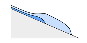
Consider a two-dimensional flow formed of two fluid layers flowing on a rigid bed  ${z = b(x)}$, where $x$ and $z$ are the horizontal and vertical coordinates (figure 1). We assume the fluids are incompressible and Newtonian, and allow their viscosities and densities to differ. We neglect surface tension and assume that no mixing between the fluid layers occurs. We refer to variables representing the upper layer using the subscript $u$ and the lower layer using subscript $l$. For layer $i$, let $\boldsymbol {u}_i = (u_i, w_i)$ denote the flow velocity, $h_i(x,t)$ the thickness, $p_i(x,z,t)$ the pressure, $\rho _i$ the density and $\mu _i$ the dynamic viscosity, where $t$ is time. The layers are each assumed to terminate at a time-dependent front with position $x=x_i(t)$.

Figure 1. Schematic illustrating the general configuration of two fluid layers flowing along an inclined rigid substrate  $b(x)$ with an upper fluid (red) of thickness $h_u(x,t)$, viscosity $\mu _u$ and density $\rho _u$ with a lower fluid (blue) of thickness $h_l(x,t)$, viscosity $\mu _l$ and density $\rho _l$. The front positions for the upper and lower layers are marked as $x_u(t)$ and $x_l(t)$, respectively.
We consider vertical-shear-dominated flow. The  $x$- and $z$-components of the lubrication equations are
 \begin{equation} \frac{\partial p_i}{\partial x} = \mu_i \frac{\partial^2 u_i}{\partial z^2}, \quad \frac{\partial p_i}{\partial z} ={-} g \rho_i, \end{equation}
respectively. The free-stress condition on the upper surface is
 \begin{equation} \frac{\partial u_u}{\partial z} = 0 \quad \text{at } z = h_u + h_l + b,\end{equation}
and the conditions of continuity on the stress and velocity at the interface read as
 \begin{gather} \mu_l \frac{\partial u_l}{\partial z} = \mu_u \frac{\partial u_u}{\partial z} \quad \text{at } z = h_l + b, \end{gather}
 \begin{gather}u_u = u_l \quad \text{at } z = h_l + b, \end{gather}
respectively. The no-slip condition at the base is
 \begin{equation} u_l = 0 \quad \text{at } z = b.\end{equation}
The model above is based on an approximation of thin layers. It should be noted that in situations where the lower fluid is much less viscous than the upper layer, we also require the viscosity ratio ( $\mu _u/\mu _l$) to be sufficiently small that the extensional stresses in the upper layer are negligible compared with the vertical shear stress.
Integrating (2.1b) and applying the continuity of pressure, we determine the pressure fields for the upper and lower fluids,
 \begin{align} p_u &= p_a + \rho_u g (h_u + h_l + b- z) \ \quad\quad \text{for} \ h_l + b < z < h_u + h_l +b, \end{align}
 \begin{align} p_l &= p_a + \rho_l g (h_l + b - z) + \rho_u g h_u \quad \text{for} \ b < z < h_l + b, \end{align}
where  $p_a$ is a constant reference pressure. On substituting (2.3) into (2.1a) and integrating the resulting differential equations subject to (2.2), the velocity profiles of each layer are
 \begin{align} u_u(x,z,t) &= \frac{\rho_u
g}{\mu_u} \left(\frac{\partial h_u}{\partial x} +
\frac{\partial h_l}{\partial x} + \frac{\textrm{d}
b}{\textrm{d} x} \right) \left[ \left( \frac{z^2 -
(h_l+b)^2}{2} \right. \right. \nonumber\\ &\hspace{11pc}
\left. \left. - (h_u + h_l + b) (z - h_l - b) \right) -
\frac{\mu_u}{\mu_l} h_u h_l \right] \nonumber\\ &\quad +
\frac{\rho_u g}{\mu_l} \left( \frac{\partial h_u}{\partial
x} + \frac{\rho_l}{\rho_u} \frac{\partial h_l}{\partial x}
+ \frac{\rho_l}{\rho_u} \frac{\textrm{d} b}{\textrm{d} x}
\right) \left( \frac{(h_l+b)^2 - b^2}{2} - (h_l + b) h_l
\right),\end{align}
\begin{align} u_u(x,z,t) &= \frac{\rho_u
g}{\mu_u} \left(\frac{\partial h_u}{\partial x} +
\frac{\partial h_l}{\partial x} + \frac{\textrm{d}
b}{\textrm{d} x} \right) \left[ \left( \frac{z^2 -
(h_l+b)^2}{2} \right. \right. \nonumber\\ &\hspace{11pc}
\left. \left. - (h_u + h_l + b) (z - h_l - b) \right) -
\frac{\mu_u}{\mu_l} h_u h_l \right] \nonumber\\ &\quad +
\frac{\rho_u g}{\mu_l} \left( \frac{\partial h_u}{\partial
x} + \frac{\rho_l}{\rho_u} \frac{\partial h_l}{\partial x}
+ \frac{\rho_l}{\rho_u} \frac{\textrm{d} b}{\textrm{d} x}
\right) \left( \frac{(h_l+b)^2 - b^2}{2} - (h_l + b) h_l
\right),\end{align}
 \begin{align} u_l(x,z,t) &=\frac{\rho_u g}{\mu_l} \left( \frac{\partial h_u}{\partial x} + \frac{\rho_l}{\rho_u} \frac{\partial h_l}{\partial x} + \frac{\rho_l}{\rho_u} \frac{\textrm{d} b}{\textrm{d} x} \right) \left( \frac{z^2 - b^2}{2} - (h_l + b) (z - b) \right) \nonumber\\ &\quad - \frac{\rho_u g}{\mu_l} \left( \frac{\partial h_u}{\partial x} + \frac{\partial h_l}{\partial x} + \frac{\textrm{d} b}{\textrm{d} x} \right) h_u (z - b). \end{align}
Both layers are driven by the component of gravity resolved along the bed, represented by the terms proportional to  $\mathrm {d}b/\mathrm {d} x$. The upper layer is also driven by the gradient in its surface slope, as represented by the sum $\partial (h_u + h_l) / \partial {x}$ in the first set of grouped terms, i.e. the first two lines of (2.4a), and moderated by interfacial stresses exerted by the lower layer, represented by the final line of (2.4a). The lower layer is likewise driven by the gradient in the weight of the fluid columns above it, represented by the terms involving $\partial h_i / \partial {x}$ in the first line of (2.4b), and couples to the upper layer through the terms involving $h_u$ and $\partial h_u / \partial {x}$.
The depth-integrated continuity equations for the two layers are
 \begin{equation}
\frac{\partial{h_i}}{\partial{t}} +
\frac{\partial{q_i}}{\partial{x}} =
0,\end{equation}
\begin{equation}
\frac{\partial{h_i}}{\partial{t}} +
\frac{\partial{q_i}}{\partial{x}} =
0,\end{equation}
where  $q_i$ denote the volume fluxes per unit width of the upper and lower layers, namely,
 \begin{equation} q_u = \int^{h_u+h_l+b}_{h_l+b} u_u \,\textrm{d} z, \quad q_l = \int^{h_l+b}_b u_l \,\textrm{d} z, \end{equation}
respectively. Substituting (2.4) into this integral, the flux expressions are
 \begin{align} q_u & ={-} \frac{\rho_u
g}{\mu_u} \left[ \left( \frac{h_u^3}{3} +
\frac{\mu_u}{\mu_l} h_u^2 h_l \right) \left( \frac{\partial
h_u}{\partial x} + \frac{\partial h_l}{\partial x} +
\frac{\textrm{d} b}{\textrm{d} x}\right) \right.\nonumber\\
&\qquad\qquad \left.+ \frac{\mu_u}{2 \mu_l} h_u h_l^2
\left( \frac{\partial h_u}{\partial x} +
\frac{\rho_l}{\rho_u} \frac{\partial h_l}{\partial x} +
\frac{\rho_l}{\rho_u} \frac{\textrm{d} b}{\textrm{d} x}
\right) \right],
\end{align}
\begin{align} q_u & ={-} \frac{\rho_u
g}{\mu_u} \left[ \left( \frac{h_u^3}{3} +
\frac{\mu_u}{\mu_l} h_u^2 h_l \right) \left( \frac{\partial
h_u}{\partial x} + \frac{\partial h_l}{\partial x} +
\frac{\textrm{d} b}{\textrm{d} x}\right) \right.\nonumber\\
&\qquad\qquad \left.+ \frac{\mu_u}{2 \mu_l} h_u h_l^2
\left( \frac{\partial h_u}{\partial x} +
\frac{\rho_l}{\rho_u} \frac{\partial h_l}{\partial x} +
\frac{\rho_l}{\rho_u} \frac{\textrm{d} b}{\textrm{d} x}
\right) \right],
\end{align}
 \begin{align} q_l & ={-} \frac{\rho_u
g}{\mu_u} \left[ \frac{\mu_u}{3 \mu_l} h_l^3 \left(
\frac{\partial h_u}{\partial x} + \frac{\rho_l}{\rho_u}
\frac{\partial h_l}{\partial x} + \frac{\rho_l}{\rho_u}
\frac{\textrm{d} b}{\textrm{d} x} \right)
\right.\nonumber\\ &\qquad\qquad \left.+
\frac{\mu_u}{2 \mu_l} h_u h_l^2 \left( \frac{\partial
h_u}{\partial x} + \frac{\partial h_l}{\partial x} +
\frac{\textrm{d} b}{\textrm{d} x} \right) \right].
\end{align}
\begin{align} q_l & ={-} \frac{\rho_u
g}{\mu_u} \left[ \frac{\mu_u}{3 \mu_l} h_l^3 \left(
\frac{\partial h_u}{\partial x} + \frac{\rho_l}{\rho_u}
\frac{\partial h_l}{\partial x} + \frac{\rho_l}{\rho_u}
\frac{\textrm{d} b}{\textrm{d} x} \right)
\right.\nonumber\\ &\qquad\qquad \left.+
\frac{\mu_u}{2 \mu_l} h_u h_l^2 \left( \frac{\partial
h_u}{\partial x} + \frac{\partial h_l}{\partial x} +
\frac{\textrm{d} b}{\textrm{d} x} \right) \right].
\end{align}
Each term can be interpreted as the ratio of a driving stress due to hydrostatic pressure gradients to a viscous resistance. The first line of (2.5c) describes the balance between the gradient in hydrostatic pressure caused by the gradient in the height of the upper interface, multiplied by (i) the variation in shear rate (the term involving  $h_u^3$) and (ii) the ‘basal drag force’ due to the resistance to shear induced in the lower layer (involving $h_u^2 h_l$). The second line represents the contribution to the flow of the upper layer induced by the gravity-driven flow of the lower layer. Equation (2.5d) is similarly structured. The first line represents the pressure gradient caused by the gradient in weight of the fluid columns arising from the variations in both the upper surface and the interface and the resistance due to the shear stress via the viscosity of the upper layer (represented by the term containing $\mu _u h_l^3/\mu _l$). In (2.5d) there is no analogue of the term representing a ‘drag force’ from the other layer (represented by the term proportional to $h_u^2 h_l$ in (2.5c)). This is because, unlike at the substrate, there is no stress exerted at the upper surface, and, hence, the upper layer experiences no resistance to moving the lower layer. The second line of (2.5d) represents the contribution to the flow of the lower layer induced by the gravity-driven flow of the upper layer. The flux expressions (2.5c,d) generalize those applying to the case of a horizontal substrate to allow for a general substrate shape $b(x)$ (note that we exactly recover the equations of Kowal & Worster (Reference Kowal and Worster2015) by setting $b=0$ and by adopting their definitions for layer thicknesses: the total thickness as $H(x,t)=h_u+h_l$ and the lower layer thickness as $h(x,t)$). The governing system of equations (2.5) allows for the existence of both two-layer regions (in which both $h_l > 0$ and $h_u > 0$) and single-layer regions in which either $h_l = 0$ and $h_u > 0$ or $h_u = 0$ and $h_l > 0$. For example, if $h_l = 0$, (2.5c) reduces to
 \begin{equation} \frac{\partial{h_u}}{\partial{t}} - \frac{\rho_u g}{\mu_u} \frac{\partial{}}{\partial{x}} \left[ \frac{h_u^3}{3} \left( \frac{\partial h_u}{\partial x} + \frac{\textrm{d} b}{\textrm{d} x}\right) \right] = 0, \end{equation}
which recovers the equation describing a single layer on a slope (Lister Reference Lister1992).
The governing equations (2.5) describe the evolution of a two-layer fluid system subject to general variations in the height of the substrate,  $b(x)$, and any given initial condition. The two-way coupling between the layers represented by the presence of both $h_u$ and $h_l$ in both flux expressions (2.5c,d) produces a rich mathematical system to be explored.
The governing equations form a parabolic initial-value problem that can be solved subject to suitable boundary conditions on the thicknesses and fluxes of the layers. At the two flow fronts, we impose
 \begin{equation} h_u(x_u,t) = 0, \quad h_l(x_l,t) = 0, \quad q_u(x_u,t) = 0, \quad q_l(x_l,t) = 0, \end{equation}
representing the independent conditions of vanishing thickness and flux at the flow fronts. Continuity conditions on flux and thickness at the transitions between single- and two-layer regions are imposed automatically by our numerical solver. The other boundary conditions will be specific to the configuration considered, e.g. an input condition on the flux or initial volume conditions, to be introduced in the relevant sections. As we will demonstrate, for flow down a slope, the system can be reduced further under the neglect of the gradients in layer thicknesses (in analogy with corresponding simplifications made in the analysis of single-layer gravity currents on inclined substrates; Mei Reference Mei1966; Fowler & Larson Reference Fowler and Larson1978; Huppert Reference Huppert1982a; Lister Reference Lister1992). This will reduce (2.5) to a hyperbolic system formed of coupled nonlinear kinematic wave equations (qualitatively similar to those proposed for coupling a glacier and its hydrological system; Fowler Reference Fowler1982), which we will detail later in § 3.3. In the special situation where the two layers have equal density ( $R=1$), the order of the flux expression (3.6c) reduces because it does not independently depend on the gradient in lower layer thickness. In our reduced asymptotic formulation our flow fronts form shocks and the imposition of zero thickness at the flow fronts is likewise abandoned. Therefore, our theory applies even in the $R=1$ situation.
3. Constant flux input of two layers
We begin by considering the situation where two fluids are introduced onto a slope at constant rates. For this, we impose the flux conditions
 \begin{equation} q_l(0,t) = q_{l0}, \quad q_u(0,t) = q_{u0}, \end{equation}
where  $q_{l0}$ and $q_{u0}$ represent the fluxes into the lower and upper layer, respectively. As a consequence of these conditions, the following integral constraints on the total volume are satisfied:
 \begin{equation} \int_0^{x_l} h_l \,\textrm{d} x = q_{l0} t, \quad \int_0^{x_u} h_u \,\textrm{d} x = q_{u0} t. \end{equation}
These expressions do not add additional constraints to this configuration (because we already have an input flux condition) but will be utilized in our later analysis. As a simple case to demonstrate the general dynamics, we assume a constant slope,
 \begin{equation} b(x) ={-} \alpha x , \end{equation}
where  $\alpha$ is a positive constant.
3.1. Intrinsic scales and dimensionless model system
In order to reduce the number of parameters in the problem, we non-dimensionalise the system using the intrinsic time, length and height scales,
 \begin{equation} \mathcal{T} = \left( \frac{\mu_u^2}{\alpha^5 \rho_u^2 g^2 q_{u0}} \right)^{{1}/{3}}, \quad \mathcal{L} = \left( \frac{q_{u0} \mu_u}{\alpha^4 \rho_u g} \right)^{{1}/{3}}, \quad \mathcal{H} = \alpha \mathcal{L} , \end{equation}
respectively. These represent the scales on which the slope of the substrate,  $\alpha = - \textrm {d} b / \textrm {d} x$, becomes important. We define non-dimensional (hatted) variables by
 \begin{equation} t = \mathcal{T} \hat{t}, \quad x = \mathcal{L} \hat{x}, \quad h_i = \mathcal{H} \hat{h}_i. \end{equation}
On dropping the hats, (2.5a) becomes
 \begin{equation} \frac{\partial h_u}{\partial t} + \frac{\partial q_u}{\partial x} = 0 \quad\text{and}\quad \frac{\partial h_l}{\partial t} + \frac{\partial q_l}{\partial x} = 0, \end{equation}
for the upper and lower layers, respectively, and the flux expressions become
 \begin{gather} q_u = \left( \frac{h_u^3}{3} + M h_u^2 h_l \right) \left( 1 - \frac{\partial h_u}{\partial x} - \frac{\partial h_l}{\partial x} \right) + \frac{M}{2} h_u h_l^2 \left( R - \frac{\partial h_u}{\partial x} - R \frac{\partial h_l}{\partial x} \right) , \end{gather}
 \begin{gather}q_l = \frac{M}{3} h_l^3 \left( R - \frac{\partial h_u}{\partial x} - R \frac{\partial h_l}{\partial x} \right) + \frac{M}{2} h_u h_l^2 \left( 1 - \frac{\partial h_u}{\partial x} - \frac{\partial h_l}{\partial x} \right), \end{gather}
where  $M = \mu _u/\mu _l$ and $R = \rho _l/\rho _u$. The boundary conditions (2.5f) become
 \begin{equation} h_u(x_u,t) = 0, \quad h_l(x_l,t) = 0, \quad q_u(x_u,t) = 0, \quad q_l(x_l,t) = 0. \end{equation}
The input conditions (3.1a,b) become
 \begin{equation} q_{l0}(0,t) = Q, \quad q_{u0}(0,t) = 1. \end{equation}
The integral constraints (3.2a,b) become
 \begin{equation} \int_0^{x_l} h_l \,\textrm{d} x = Q t, \quad \int_0^{x_u} h_u \,\textrm{d} x = t. \end{equation}
The dimensionless model above depends on three dimensionless parameters,
 \begin{equation} M = \frac{\mu_u}{\mu_l}, \quad R = \frac{\rho_l}{\rho_u}, \quad Q = \frac{q_{l0}}{q_{u0}}, \end{equation}
representing the ratios of viscosity, density and input flux, respectively.
Cases of  $M > 1$ represent configurations where the lighter fluid is more viscous than the heavier fluid. In such cases, (3.6) is structurally similar to the coupled kinematic wave equations that Fowler (Reference Fowler1982) applies to describe the two-way interplay between a glacier and its hydrological system; the main difference being that the flux expressions that Fowler (Reference Fowler1982) develop depends on interstitial water flux while ours depend on layer thicknesses. Additionally, our study offers a preliminary framework for understanding more complicated rheologies for the lower layer, such as a granular medium (like till) beneath a power-law viscous glacier.
3.2. Illustration of phenomena
To illustrate the general dynamics, we begin by presenting a series of numerical solutions to the dimensionless model (3.6). For this, we used a finite-volume numerical scheme based on converting the conservative form of the partial differential equations to surface integrals and solving them by evaluating the flux into and out of ‘cells’ (small volumes) at each spatial node (e.g. LeVeque Reference LeVeque1992). The details of the scheme are provided in Appendix A. Note that the global volume constraint and continuity of flux and velocity at the lower layer flow front are automatically satisfied by this numerical method. The finite-volume method is particularly suited to the system (2.5) because it can resolve steep gradients, is automatically mass conservative and remains stable during the development of any shock fronts (such as configurations where  $R=1$). Despite these advantages, few studies of thin-film dynamics use finite-volume schemes (one example is Grün, Lenz & Rumpf Reference Grün, Lenz and Rumpf2002) and our application here demonstrates in particular its effectiveness for multi-layer fluid flows.
Two illustrative examples are shown in figure 2. For example A, we set  $M=10$ (corresponding to the upper fluid being ten times more viscous than the lower fluid) and for example B, we set $M=0.1$ (corresponding to the lower fluid being ten times more viscous than the upper fluid). In each, $R=2$ and $Q=0.5$. Time slices of each solution are shown at a progression of times, $t=1$ and 10, in figure 2(a,b,d,e). The evolutions of the flow fronts are illustrated in figure 2(c,f).

Figure 2. Illustrative numerical solutions to the full dimensionless model (3.6) for the situation where two fluids are injected continuously. In example A (panels a–c) the viscosity ratio is  $M = 10$, corresponding to the upper layer being ten times more viscous than the lower layer (forming a lubricating film). In example B (panels d–f) $M = 0.1$, corresponding to the upper layer being ten times less viscous than the lower layer. In both, the flux ratio is $Q = 0.5$ and the density ratio is $R = 2$. Profiles show the solutions at $t=1$ (a,d), $t=10$ (b,e). Panels (c,f) show the evolution of the two flow fronts, $x_u(t)$ and $x_l(t)$, towards linear growth. The inset in (c) shows the convergence of the numerical solutions to the asymptotic theory $900<t<1000$.
The solution for example A illustrates the development of two distinct flow regions. Upstream, the flow forms a region containing both fluid layers. Beyond a critical position, the lower layer terminates and the flow forms a downstream region comprised purely of the lighter fluid. In this example, the thickness of the downstream single-layer region is larger than that of the two-layer region, with a shock-like transition between the two. The plot of the frontal evolutions in figure 2(c) indicate that the fronts propagate at a constant speed at late times, such that the length of the two-layer region approaches a fixed proportion of the length of the total flow. For example B, the upper layer is instead ten times less viscous than the lower layer. The flow likewise forms two regions comprising a region of lighter fluid extending ahead. A key difference compared with example A is that the thickness of the downstream single-layer region is now thinner than the total thickness of the upstream two-layer region. The front positions in case B again transition towards linear growth (figure 2f), showing that the distance between the fronts continues to grow to late times.
The solutions have illustrated a number of universal features. One is that a two-layer release always forms a two-region structure in which the lighter fluid extends ahead of the heavier fluid. Another is that the flow fronts approach linear growth at long times. The solutions also illustrate that it is possible for the frontal thickness to be either greater than or less than the total thickness of the two-layer region. Our analysis will determine solutions describing the long-term asymptotic flow. To this end, we split the analysis into two components. First, we investigate the independent question of how the thickness of the layers in the two-layer region are controlled. With this analysis in hand, we consider the full system comprising both the two-layer region and the frontal region.
3.3. Two-layer region
Our numerical solutions of (3.6) indicated that the solutions approach steady-state thicknesses over time. To confirm this, in figure 3 we plot the thicknesses of both fluid layers as a function of time at the position  $x=10$. The lighter fluid front passes first through this point, followed by the two-layer region. By $t=10$ in figure 3(a) and by $t=50$ in figure 3(b), the layer thicknesses in the two-layer region converge to steady-state values. We compare the time-dependent layer thicknesses from the numerical solutions in figure 2 at $x=10$ to the theoretical thickness values (obtained under a steady-state approximation of (3.6), whose calculation we describe in this section) and find agreement. This confirms the approach of the upstream two-layer region to a steady state, whilst also corroborating the validity of our numerical solver and the validity of the steady-state approximation.

Figure 3. Thicknesses of the individual fluid layers at the fixed position  $x=10$, showing the convergence of the numerical solutions in the upstream two-layer region towards steady values. Thicknesses plotted here are from our full numerical simulations shown in figure 2 for the following dimensionless parameters: $R=2$, $Q=0.5$ and (a) $M=10$, (b) $M=0.1$. The numerical lower layer thickness is represented by the thin blue line and the numerical upper layer thickness by the thin red line. The steady-state thicknesses predicted by the theory in (3.7) are overlaid in thick black lines.
Integrating the steady-state forms of (3.6a–c) subject to (3.6e), we obtain
 \begin{align} 1 &= \frac{h_u^{3}}{3} + M h_u^{2} h_l + \frac{MR}{2} h_l^2 h_u, \end{align}
 \begin{align}Q &= M \left( \frac{R}{3} h_l^3 + \frac{1}{2} h_u h_l^2 \right). \end{align}
Since these equations are independent of  $x$, it follows that the thicknesses of the layers, $h_u$ and $h_l$, are spatially uniform, confirming the form indicated by our numerical solutions (figures 2 and 3). It should be noted that, in deriving the algebraic equations above, we did not impose the condition that the layers are uniform, only the weaker assumption that the gradient in thicknesses of the layers tends to zero. Since the equations are purely algebraic on neglect of these gradients, it follows that the long-term asymptotic state of the layers is spatially uniform. To solve the equations above, we could use (3.7b) to eliminate $h_u$ in (3.7a) to obtain a cubic equation for $h_l^3$. Since the order of the equation is odd, it is guaranteed to have at least one real root. In order to conduct a complete parameter sweep over values of $M$ and $Q$ using parameter continuation, we opt to solve for $h_u$ and $h_l$ in (3.7) numerically using a Newton–Raphson iterative solver. In doing this, the closest real, positive solution found previously by the solver is used as an initial guess for the next value. There is only one root for which both $h_u$ and $h_l$ are real and positive (and, therefore, physically relevant). As a general point of contrast, we note that previous studies of multi-layered gravity currents have required considerably more detailed analysis of differential systems with unknown free-parameters (cf. Woods & Mason Reference Woods and Mason2000; Kowal & Worster Reference Kowal and Worster2015; Pegler et al. Reference Pegler, Huppert and Neufeld2016). The reduction of our governing equations (3.6) to a simple coupled algebraic system demonstrates both the analytical tractability of the present problem and, as we will show below, will establish a new basis for regime classification of such flows based on the dynamics of the two-layer region alone.
We begin by considering the effect of the viscosity ratio  $M$. In our dimensionless model $M$ represents the dimensionless viscosity of the upper layer, whilst the viscosity of the lower layer is fixed at unity. Figure 4(a) shows the thicknesses of the two layers, $h_l$ and $h_u$, as functions of $M$, with $Q=0.5$ and $R=2$ each held fixed. At small values of $M$ (for which the upper layer has a very small viscosity), both layer thicknesses asymptote to the thicknesses that would apply if the layers were considered in isolation, namely,
 \begin{equation} h_l \sim \left( \frac{3Q}{MR} \right)^{1/3}, \quad h_u \sim 3^{1/3}, \end{equation}
for  $M \to 0$. The approach of the upper layer towards its single-layer thickness (3.8b) can be understood by noting that, in view of its small viscosity, the upper layer is much thinner than the lower layer and, therefore, exerts a negligible stress on it. The upper layer therefore has no effect on the lower layer. Conversely, the small viscosity of the upper layer means that the lower layer is effectively static relative to the speed of the upper layer, and, thus, acts as a rigid surface for the upper layer. In this limit, the lighter fluid therefore flows effectively as a single layer over the top of the more viscous heavier fluid. We refer to this situation as regime C.

Figure 4. Thicknesses of the two layers,  $h_u$ and $h_l$, with fixed $R=2$ for the case of varying (a) viscosity ratio $M=\mu _u/\mu _l$ and (b) input flux ratio $Q=q_{l0}/q_{u0}$. Here, $h_i$ denotes the steady-state thicknesses for layer $i$. The fixed parameters are: (a) $Q = 0.5$; (b) $M = 1$. The numerical solutions of (3.7) are represented by the thin blue (lower layer) and red (upper layer) solid lines. The asymptotes are overlaid in thick black dashed lines. Layer thicknesses are equal when $M=1$ in panel (a) and when $Q = 1/2$ in panel (b).
As  $M$ is increased, the thicknesses of the two layers approach comparable values for $M=O(1)$. For large $M$, both layers thin together as $M^{-1/3}$ (figure 4a). For the lower layer, this decrease follows the trend established from the small $M$ limit (albeit with a different prefactor) and is consistent with the layer flowing faster as its viscosity is reduced. The concurrent decrease in the thickness of the upper layer as $M^{-1/3}$ instead differs from its small- $M$ trend. The decrease is an effect of the lubrication provided by the lower layer: the reduction in underlying shear stress caused by lubrication increases the flow rate of the upper layer and, to maintain the same flux, results in a thinner layer. For $M \to \infty$, we can neglect all terms in (3.7) except those multiplied by $M$. Solving the resulting simplified system, we obtain the asymptotic predictions
 \begin{equation} h_l \sim \frac{\psi(QR)}{(MR^2)^{1/3}} , \quad h_u \sim \frac{\phi(QR)}{(M/R)^{1/3}}, \end{equation}
for  $M \to \infty$, where the functions
 \begin{align} \psi(\xi) &\equiv \left[ \frac{3}{2} \left( 5 \xi - \left[ (3 \xi + 5)^2 - 16 \right]^{1/2} + 3 \right) \right]^{1/3}, \end{align}
 \begin{align}\phi(\xi) &\equiv \psi(\xi) \left( \frac{2\xi}{\psi(\xi)^3} - \frac{2}{3} \right). \end{align}
The results of (3.9) are shown as dashed black lines in figure 4(a) and confirm the mutual  $M^{-1/3}$ thinning trends. Via the functions of $\phi (QR)$ and $\psi (QR)$, the large- $M$ limit retains a relatively complex dependence of the layer thicknesses on the flux ratio $Q$. The parameter $Q$ can be interpreted as the dimensionless flux inputted into the lower layer, whilst the dimensionless flux inputted into the upper layer is fixed at unity. As shown in figure 5, $\psi$ and $\phi$ are increasing and decreasing functions, respectively. The former is consistent with the anticipated thickening of the lower layer as the flux $Q$ introduced into it is increased. The latter implies that the thickness of the upper layer decreases as the flux inputted into the lower layer is increased. This applies because increasing $Q$ results in more lubrication, reducing the stress on the upper layer and causing it to flow faster. Since the input flux is fixed, the faster flow rate results in a thinner upper layer.

Figure 5. The functions  $\psi (\xi )$ and $\phi (\xi )$ defined by (3.9c,d) arising in the large- $M$ asymptotic theory for the thicknesses of two fluid layers on a slope, $h_u$ and $h_l$. Asymptotes are overlaid as black dashed lines.
We note that the  $M\to \infty$ limit in (3.9) encompasses limits of small and large input flux ratio $Q$. In the limit $QR \to 0$, (3.9) reduces to
 \begin{equation} h_l \sim \left( \frac{4 Q^2}{M} \right)^{{1}/{3}}, \quad h_u \sim \frac{1}{(2QM)^{{1}/{3}}}, \end{equation}
confirming that the upper layer thickens as  $Q^{2/3}$ and the lower layer thins as $Q^{-1/3}$ as $Q$ is increased, both of which are indicated by the increasing and decreasing functions of $\psi$ and $\phi$, respectively (figure 5). We name this situation regime A. We can likewise reduce (3.9) in the limit $QR \to \infty$ which asymptotes to
 \begin{equation} h_l \sim \left( \frac{3Q}{MR} \right)^{1/3}, \quad h_u \sim \frac{2}{(9 M Q^2 R)^{1/3}}. \end{equation}
In this limit the lower layer grows in proportion to  $Q^{1/3}$ whilst the upper decreases in proportion to $Q^{-2/3}$. As $Q \to \infty$, the upper fluid layer is very thin and has negligible impact on the lower layer. The lower layer therefore approaches the thickness it would have in isolation, which is consistent with (3.11a). The upper layer simply translates with the top of the lower layer at the velocity $u_u = MR h_l^2/2$, where $h_l$ is given by (3.11a). The combination of this expression with the flux constraint, $h_u u_u = 1$, indeed produces (3.11b). We refer to this situation as regime D.
To illustrate the effect of the flux ratio  $Q$, we plot $h_u$ and $h_l$ as functions of $Q$ in figure 4(b) for $M=1$ and $R=2$. For $Q \to 0$, (3.7) yields the asymptotic predictions
 \begin{equation} h_l \sim \left( \frac{2Q}{3^{1/3} M} \right)^{1/2}, \quad h_u \sim 3^{1/3}, \end{equation}
which we have plotted as dashed lines in figure 4(b). The thickness of the upper layer asymptotes to the value that would apply if it were in isolation (3.12b), implying a negligible effect of the lower layer on the upper in this limit. Equation (3.12a) shows that the lower layer assumes a small thickness proportional to  $Q^{1/2}$. To understand this, we note that, for $Q \to 0$, the lower layer forms a thin Couette flow with a shear rate controlled by the stress applied at the base of the upper layer. More specifically, the stress continuity condition (2.2b) implies that the shear rate is $M \partial u_u / \partial {z}$, where $\partial u_u / \partial {z} = 3^{1/3}$ is the shear rate of the upper layer near the base, resulting in a leading-order velocity profile of $u_l = 3^{1/3}Mz$ in the lower layer. Integrating this shear profile over the depth of the lower layer and applying the flux constraint $q_l = \int u_l \,\textrm {d} z = Q$, we obtain (3.12a). This situation is referred to as regime B.
As  $Q$ is increased to values of order unity, the two layers approach comparable thicknesses. For $Q \to \infty$, we recover the asymptotes (3.11) in regime D which are shown to agree with our numerical predictions in figure 4(b). That there are two routes to deriving (3.11), one involving the reduction of (3.7) and one involving the general expression for the $M \to \infty$ limit, indicates that (3.11) describes a limit that encompasses all values of $M$ for sufficiently large $Q$, and this will be illustrated in § 3.5.
To visualise all the configurations of a two-layer gravity current on a single parameter–regime diagram, we present in figure 6 a map of the  $(M,Q)$ parameter space divided into four regions by four curves. These regimes are determined by evaluating when the Newton–Raphson numerical solutions for the layer thicknesses in (3.7) fall within 10 % of the theoretical predictions in table 1. The unshaded regions in the $(M,Q)$ parameter space represent parameters over which the system transitions between these regimes. The asymptotes describing the partitioning curves between these regimes are annotated. Regime A (in red) falls within the curves $M \gg 1/6Q$ and $Q \ll 3/4R$ and represents the region in which the numerical solutions fall within 10 % of the asymptotic prediction for the simultaneous limits $M\to \infty$ and $Q\to 0$ (3.10). In regime A the layer thicknesses in the two-layer region thin as $M^{-1/3}$. Regime B is represented by the purple region $8QR^2/27 \ll M \ll 1/6Q$, describing the ‘rigid-lid regime’ in which $Q\to 0$. In this regime the upper layer thickness asymptotes to the value that would apply if it were in isolation and the lower layer forms a thin Couette flow at the base of the upper layer. Regime C (in green) falls within $8QR^2/27 \ll M \ll 8/27Q^2R$ and describes the region in which the numerical solutions lie within 10 % of the asymptotic prediction for the $M \to 0$ limit (3.8). In this regime both layer thicknesses in the two-layer region asymptote to the value that would apply if the layers were released in isolation. Regime D falls in the remaining blue region $Q \gg 3/4R$ and $M \gg 8/27Q^2R$ where the numerical solutions fall within 10 % of the asymptotic predictions for the $Q\to \infty$ limit (3.11). In this regime the lower layer acts as a ‘conveyor belt’ on top of which the upper layer translates. This regime covers a significant region of the parameter space, encompassing asymptotic limits involving both large and small $M$. The structure produces a thick region of heavier fluid in the two-layer region.

Figure 6. Universal regime diagram illustrating the configurations of a two-layer fluid flow introduced at a constant flux onto an inclined plane for  $R=2$. The diagram is constructed by determining where the Newton–Raphson numerical solutions for the layer thicknesses from (3.7) fall within 10 % of the asymptotic thickness predictions in table 1. The parameter space of $(M, Q)$ is partitioned into four regimes. Regime A (red region) describes the region in which layer thicknesses mutually thin as $M^{-1/3}$. Regime B (purple region) describes the limit in which the upper layer thickness asymptotes to the value that would apply if the layer was released in isolation. Regime C (green region) describes the region in which the thicknesses of both fluid layers asymptote to the values that would apply if the layers were released in isolation. Regime D (blue region) describes a region that encompasses a wide range of $M$ and $Q$. The blue line marks the demarcating boundary $h_l=h_u$.
Table 1. Predictions for layer thicknesses in the two-layer region (§ 3.3) in each of the four regimes A, B, C and D that are identified in figure 6.

To visualise the control of the relative thicknesses of the two layers in this parameter–regime diagram, we also plot in blue the curve along which the thicknesses in the two-layer region are equal to each other and by setting  $h_u = h_l$ in (3.7), we determine the exact seperatrix between these two configurations to be $M = 2Q/(3+2R-6Q-3QR)$. The diagram shows that for $M \gtrsim 1$, the ratio of thicknesses is controlled almost independently by the flux and density ratios alone. An interesting feature is that if the flux ratio is sufficiently large, $Q > (3+2R)/(6 + 2R)$, the lower layer is certain to be thicker than the upper layer, irrespective of the value of the viscosity ratio $M$. Regimes A and B have a thicker upper layer and regimes C and D have a thicker lower layer. We establish a simple demarcation between these pairs of regimes based on layer thicknesses.
Remarkably, the results above show that the dynamics of inclined two-layer gravity currents can be classified entirely from the thicknesses in the two-layer region (3.7). These regimes are not necessarily associated with finite fluid layers. Notably, we emphasise the equivalence of the  $M,Q$ scalings that define the demarcations of the regimes in figure 6 and the regimes in Kowal & Worster (Reference Kowal and Worster2015). Unlike previous work, we have derived full asymptotic conditions, including prefactors and dependence on the density ratio $R$. The second crucial distinctions between the regimes in these two studies arises from the scalings in the evolution equations for layer thicknesses and front positions: the horizontal substrate thicknesses scale as $1/5$-powers in $M$ and $Q$, while the inclined substrate thicknesses scale as $1/3$-powers. That said, their regime I (describing situations in which the upper layer has a higher viscosity and a higher input flux than the lower layer and spreads under its own weight) shares similarities with our regime B, in which the lower layer forms a Couette flow due to the stress applied at the base of the upper layer. The theoretical predictions we obtain for regime B (table 1) are identical to the scalings for thickness in regime I of their study. We note that despite the similarities between their regime I and our regime B, the analytical reductions differ. In view of the fundamental difference between the two problems, we show that our coupled cubic algebraic equations (3.7) likely underlie the regimes of all two-layer flows.
3.4. Initiation of two-layer fluids into an empty domain
Having understood the independent dynamics of the two-layer region, we are in a position to construct solutions to the problem in which two finite layers are released and form independently propagating flow fronts.
At long times, the flow becomes increasingly slender as it extends down-slope. Therefore, the thickness gradients  $\partial h_i / \partial {x}$ become progressively smaller relative to $\mathrm {d} b/\mathrm {d} x$ in the governing flux expressions (3.6b,c) as $t$ increases. Thus, at long times, we assume that the along-slope component of gravity (represented by $\textrm {d} b / \textrm {d} x$) provides the dominant contribution. In dimensionless forms, these expressions reduce to
 \begin{align} \frac{\partial h_u}{\partial t} + \frac{\partial q_u}{\partial x} &= 0, \quad q_u = \frac{h_u^3}{3} + M h_u^2 h_l + \frac{MR}{2} h_u h_l^2 , \end{align}
 \begin{align}\frac{\partial h_l}{\partial t} + \frac{\partial q_l}{\partial x} &= 0, \quad\, q_l = \frac{MR}{3} h_l^3 + \frac{M}{2} h_u h_l^2. \end{align}
Equation (3.13a) describes the flux of the upper layer where each term represents contributions from shear variations of the upper layer itself, from the basal stress acting on the upper layer and from the drive induced by the motion by the lower layer, respectively. Equation (3.13b) represents the flux of the lower layer with contributions from flow induced by the motion of the upper layer and from the shear variations in the lower layer, respectively.
By conducting a scaling analysis of the system, we obtain the scalings of  $h/t \sim h^3/x$ from (3.13) and $hx \sim t$ from (3.6e) which are consistent with previous studies of single-layer flows on slopes (e.g. Huppert Reference Huppert1982a; Lister Reference Lister1992). Combining these, we obtain $x \sim t$ and $h \sim 1$. These scalings differ from those arising for constant flux inputs over horizontal substrates, where the propagation rates go as $t^{1/5}$ (Huppert Reference Huppert1982b; Kowal & Worster Reference Kowal and Worster2015).
The scaling analysis above indicates the existence of similarity solutions of the form  $h =h(\eta )$, where
 \begin{equation} \eta = t^{{-}1}x, \end{equation}
with front positions  $x_u = \eta _u t$ and $x_l = \eta _l t$, where $\eta _u$ and $\eta _l$ are constants. The similarity scaling implies that the flow becomes increasingly slender at long times, $\partial h / \partial {x} \sim 1/t$, thus confirming that the approximation of neglecting $\partial h / \partial {x}$ is self-consistent. Recasting (3.6) in terms of the similarity coordinate (3.14), the equations reduce simply to $\mathrm {d} q_i/\mathrm {d} \eta = 0$, where $q_i$ are given by (3.13). Thus, the fluxes through both layers are uniform through the length of the similarity solutions. Integration of $\mathrm {d} q_i/\mathrm {d} \eta = 0$ subject to the input conditions (3.6e) yields
 \begin{gather} \frac{h_u^{3}}{3} + M h_u^{2} h_l + \frac{MR}{2} h_l^2 h_u = 1, \end{gather}
 \begin{gather}M \left( \frac{R}{3} h_l^3 + \frac{1}{2} h_u h_l^2 \right) = Q. \end{gather}
These expressions are equivalent to those arising in our analysis of steady two-layer flows in § 3.3. The equivalence reflects a property of the similarity solutions considered here, namely, that the height profiles that conform to the similarity scalings are steady (inherent in the scaling  $h \sim 1$). The time dependence of the flow therefore arises entirely from the evolution of the moving flow fronts, $x_l(t)$ and $x_u(t)$.
Within the upstream region comprising both fluid layers,  $0 < \eta < \eta _l$, we apply (3.15) to calculate the thicknesses of the two layers. This forms a component of the similarity solution that is equivalent to the problem explored in § 3.3. To determine the thickness in the downstream region comprising the lighter fluid alone, $\eta _l < \eta < \eta _u$, we set $h_l = 0$ in (3.15a) to obtain
 \begin{equation} h_u = 3^{1/3}. \end{equation}
The heights in the two regions can thus be determined from (3.15) before the extents of these regions  $\eta _l$ and $\eta _u$ are known.
The integral constraints (3.6f) yield
 \begin{equation} \int_0^{\eta_l} h_l \, \mathrm{d} \eta = Q, \quad \int_0^{\eta_l} h_u \, \mathrm{d} \eta + \int_{\eta_l}^{\eta_u} 3^{1/3} \, \mathrm{d} \eta = 1, \end{equation}
where we have substituted for the thickness in the single-layer region using (3.15c). Since  $h_l$ and $h_u$ are uniform, these expressions reduce to
 \begin{equation} \eta_l = \frac{Q}{h_l}, \quad \eta_u = \eta_l + 3^{{-}1/3} \left(1 - \frac{Q h_u}{h_l} \right), \end{equation}
giving explicit formulae for the positions of the flow fronts  $\eta _l$ and $\eta _u$ in terms of the known thicknesses $h_l$ and $h_u$ given by (3.15). It is evident from the similarity solutions (3.17) that the upper fluid always extends ahead of the lower layer to form a single-layer region in front of a two-layer region, confirming our observation from the numerical solutions in figure 2. This essential structure can be understood by noting that, in the two-layer region, the lighter fluid must always flow at least as fast as the heavier fluid below it (its speed is given by the speed of the top surface of the lower layer plus an additional contribution due to the slope of its upper surface). Therefore, the lighter upper fluid must eventually flow ahead of the heavier lower fluid to form a secondary, independent single-layer region.
The similarity solutions can be constructed systematically as follows. First, we determine the thicknesses in the two-layer region,  $h_l$ and $h_u$, by solving (3.15a,b) using the Newton–Raphson solver applied in § 3.3. The length of the upstream region $\eta _l$ can then be evaluated using (3.17a). The volume of the lighter fluid in the two-layer region can be determined as $\eta _l h_u$, leaving a residual volume of $1-\eta _l h_u$ to extend ahead and form the single-layer region. Equating the cross-sectional area of the downstream region with this residual, $3^{1/3} (\eta _u - \eta _l) = 1 - \eta _l h_u$ and rearranging, we obtain (3.17b).
Two illustrative solutions are shown in figure 7. For these, we apply the same parameter settings used for our two numerical examples shown earlier in figure 2. We note that while the similarity solutions predict a discontinuity in thickness at the lower layer flow front, in the full unsimplified model (3.6), the higher-order diffusive contributions intervene to smooth the discontinuities (cf. a single-layer flow on a slope Lister Reference Lister1992). The solutions exhibit differences in the thicknesses and lengths of the two regions. While the thickness of the single-layer region is universal, the total thickness of the two-layer region can either be greater than or less than the thickness of the single-layer region. The predictions for the frontal positions,  $x_u = \eta _u t$ and $x_l = \eta _l t$, are shown as dashed lines in figure 2(c,f), where they are shown to successfully match our numerically determined predictions at long times.


3.5. The control of the propagation rate
In order to understand the general parametric control of the flow structure predicted by the system of (3.15) and (3.17), we have plotted the positions of the layer fronts,  $\eta _u$ and $\eta _l$, as functions of the viscosity ratio $M$ for fixed values of $Q=0.5$ and $R=2$ in figure 8(a). The corresponding length of the single-layer region, $\eta _l - \eta _u$, is shown in figure 9(a). As $M$ is increased, $\eta _u$ and $\eta _l$ both increase, which is consistent with both layers propagating faster as the viscosity of the lower layer is reduced. For small $M$, we substitute the asymptotic results of the two-layer region given by (3.8) into (3.17) to give the frontal positions
 \begin{equation} \eta_l \sim \left( \frac{MRQ^2}{3} \right)^{1/3}, \quad \eta_u \sim \eta_l + 3^{{-}1/3}, \end{equation}
as  $M \to 0$. In this limit, the two-layer region is considerably thicker and shorter than the single-layer region. In effect, the heavier fluid acts as a near-rigid, narrow topographic obstruction for the lighter fluid between $\eta = 0$ and $\eta _l$. Once the lighter fluid flows over this, its extent is then effectively equivalent to that which would apply if it were in isolation, forming a dimensionless length of $3^{-1/3}$.

Figure 8. Numerical solutions of the front positions in (3.17) (thin unbroken lines) overlaid by their asymptotes (thick dashed lines) for fixed  $R=2$ over a wide range of the (a) viscosity ratio $M$ and (b) the flux ratio $Q$. The fixed parameters are (a) $Q=0.5$ and (b) $M=1$. In panel (a) the function $\zeta (QR) = 3^{-1/3}[1 - QR \phi (QR)/\psi (QR)]$, as defined by (3.19c).

Figure 9. The length of the frontal (single-layer) region  $\eta _u-\eta _l$ overlaid with its asymptotes for fixed $R=2$ over a wide range of (a) the viscosity ratio $M$ (fixed $Q=0.5$) and (b) the flux ratio $Q$ (fixed $M=1$). The plots illustrate the approach of the length towards constants in each limit. In panel (a) the grey rectangle indicates the range of possible values spanned by $\zeta (QR)$. The inset in panel (a) plots the function $\zeta (QR)$ defined by (3.19c), representing the dimensionless length in the limit $M \to \infty$.
For  $M \to \infty$, the length of the two-layer region becomes comparable to the length of the full system. Substituting (3.9) into (3.17), we obtain
 \begin{equation} \eta_l \sim \frac{Q (MR^2)^{1/3}}{\psi(QR)}, \quad \eta_u \sim \eta_l + \zeta(QR), \end{equation}
for  $M \to \infty$, where
 \begin{equation} \zeta(QR) \equiv 3^{{-}1/3}\left( 1 - QR \frac{\phi(QR)}{\psi(QR)} \right) \end{equation}
is a function of  $QR$ alone, representing the length of the single-layer region. The front position of the two-layer region thus grows as $M^{1/3}$, representing the acceleration of the rate of propagation by lubrication. By contrast, the length of the single-layer region approaches a constant $\zeta (QR)$ that is independent of $M$. The value of $\zeta (QR)$ across the entire range of $QR$ is strictly bounded within the narrow range $2 < 3^{1/3} \zeta < 3$. The extent of this band of values is indicated by the grey shaded rectangle in figure 9(a). Since $\eta _u - \eta _l$ must also asymptote to the universal value $3^{-1/3}$ as $M \to 0$, the dimensionless length of the frontal region is an almost universal function of the viscosity ratio $M$ alone.
As shown in figure 9(b), both layers grow as the flux ratio  $Q$ is increased. For $Q \to 0$, we substitute (3.12) into (3.17) to give
 \begin{equation} \eta_l \sim \left( \frac{3^{1/3}}{2} MQ \right)^{1/2}, \quad \eta_u \sim 3^{{-}1/3}. \end{equation}
The two-layer region thus occupies a short region of length  $Q^{1/2}$ in front of the source, while the flow is primarily comprised of the lighter fluid. As $Q$ increases, the two-layer region develops and eventually dominates the flow domain. The upper layer front position is asymptotically described only by the propagation of this lower layer frontal region. For $Q \to \infty$, we substitute (3.11) into (3.17) to give
 \begin{equation} \eta_l \sim \left( \frac{MRQ^2}{3} \right)^{1/3}, \quad \eta_u \sim \eta_l + 3^{{-}4/3}, \end{equation}
showing that the extent of the two-layer region (and, thus, of the entire flow) grows as  $Q^{2/3}$. As illustrated in figure 9(b), the length of the single-layer region approaches the universal asymptotic value $\eta _u-\eta _l \sim 3^{-4/3}$, equal to one third of the length predicted by single-layer theory, e.g. (3.20b). Remarkably, for large input flux of the heavier fluid, the lighter fluid will always partition its volume such that $2/3$ of it lies in the two-layer region while the remaining $1/3$ lies in the frontal region. This property applies universally for all $M$ and $R$, assuming large $Q$. As a result, the thickness and length of the single-layer region is almost entirely insensitive to the specific value of all the dimensionless parameters.
We compare the convergence of the front positions of the numerical solutions towards the asymptotic predictions determined here (figure 2c,f). In both cases, the numerical solutions converge to the theoretical prediction. There is exact agreement between the prediction for both layers’ front position in the case of  $M=0.1$ and between the prediction for the lower layer front position in the case of $M=10$. The result for $M=10$ shows that the front of the upper layer takes relatively longer to approach the asymptotic prediction of the reduced theory, as compared with the lower layer front (as indicated by the inset of figure 2c). This is likely because of the considerably larger viscosity of the upper layer, which acts to increase the time it takes for the layer to adjust to its corresponding asymptotic prediction. Conversely, when the lighter fluid is much less viscous than the heavier fluid ( $M=0.1$), the convergence of the front position of the lighter fluid is relatively faster.
Our description of the four regimes in figure 6 is now enriched with information gained from our finite layer analysis. A summary of the front position predictions in each regime are presented in table 2, building on the summary of partitioning curves and layer thickness predictions in table 1. In regime A the structure involves a region of lubrication connected to a thick region of lighter fluid forming the nose. In this case, the lubricating region acts as a ‘bulldozer’, pushing the relatively larger quantity of more viscous fluid considerably further than it would spread in isolation. (In this instance, a horizontal pressure gradient drives the system forward, transferring the lubricating lower layer velocity to the single-layer region.) Regime B describes a configuration in which the lighter fluid layer occupies a considerable proportion of the length of the two-layer system. In contrast to the configuration in regime A, the structure in regime C produces a thin region of lighter fluid that extends downstream of the heavier fluid front. In regime D the structure produces a thick region of heavier fluid upstream of a thin single-layer region. Single-layer frontal regions that are thicker and thinner than the upstream two-layer region fall within this region.

4. Fixed volume release of two layers
We consider now the situation where two fluid volumes are released together onto an inclined surface. In this case, we assume the layers are initialised with profiles  $h_u(x,0)$ and $h_l(x,0)$, with volumes prescribed by the integral constraints,
 \begin{equation} \int_0^{x_l} h_l \,\textrm{d} x = v_{l0}, \quad \int_0^{x_u} h_u \,\textrm{d} x = v_{u0}, \end{equation}
where  $v_{u0}$ and $v_{l0}$ are the volumes of the upper and lower layers, respectively. We also assume that no fluid enters the domain at $x=0$ by imposing
 \begin{equation} q_u(0,t) = 0, \quad q_l(0,t) = 0, \end{equation}
which can be interpreted as a no-penetration condition or symmetry condition at  $x=0$.
4.1. Intrinsic scales and dimensionless model system
We non-dimensionalise the system using the intrinsic time, length and height scales,
 \begin{equation} \mathcal{T} = \left( \frac{\mu_u^2}{\alpha^5 \rho_u^2 g^2 v_{u0}} \right)^{1/2}, \quad \mathcal{L} = \left( \frac{\alpha \rho_u g \mathcal{T} v_{u0}^2}{\mu_u} \right)^{1/3}, \quad \mathcal{H} = \alpha {\mathcal{L}}. \end{equation}
We define dimensionless (hatted) variables according to
 \begin{equation} t = \mathcal{T} \hat{t}, \quad x = \mathcal{L} \hat{x}, \quad h_i = \mathcal{H} \hat{h}_i, \end{equation}
The dimensionless governing equations are identical to (3.6a–d). The only difference is that we now impose the volume constraints (4.1) and the flux conditions (4.2), the former taking the dimensionless forms
 \begin{equation} \int_{0}^{x_u} h_{u} \,\textrm{d} x = 1, \quad \int_{0}^{x_l} h_{l} \,\textrm{d} x = V, \end{equation}
where  $V = v_{l0}/v_{u0}$. The dimensionless system above depends on three dimensionless parameters
 \begin{equation} M = \frac{\mu_u}{\mu_l}, \quad R = \frac{\rho_l}{\rho_u}, \quad V = \frac{v_{l0}}{v_{u0}}, \end{equation}
the ratios of viscosity, density and fluid volumes, respectively.
4.2. Illustration of phenomena
We illustrate the general behaviour using our numerical solver in figure 10. To initialise the layers, we introduce them into an initially empty domain at constant dimensionless fluxes ( $q_u = 1$ and $q_l = V$) over the short interval $-1 < t < 0$. The input was terminated at $t=0$, producing fixed volumes for all subsequent times, $t > 0$, in accordance with (4.5). We show two example viscosity ratios given by (A) $M=10$ and (B) $M=0.1$, with $R=2$ and $V=0.5$. Each evolution is shown as a progression of time slices at $t=1$ (figure 10a,d) and $t=10$ (figure 10b,e). In both examples, the thickness of the lighter fluid above the heavier fluid thins progressively, to the extent that the two fluids largely occupy independent layers at long times. This can be understood by noting that the fluid on top of the lower layer always flows faster than the lower layer and, hence, without a resupply of lighter fluid, the upper layer progressively ‘spills’ ahead the heavier fluid. The lighter fluid always advances ahead of the heavier fluid because its speed is at least as fast as the top surface of the heavier fluid below it. In contrast with example A, in case B the lighter fluid front is consistently thinner than the heavier fluid upstream of it. There is a drop, rather than a jump, in thickness at the front of the heavier fluid at large times. A second key difference between the examples is the extent of each fluid. The heavier fluid is longer in case A than it is in case B and the lighter fluid is longer in case B than in case A. This suggests that, despite the separation of the flows, the less viscous layer plays a key role in propagating the frontal region of lighter fluid. In contrast to the constant flux case, the front positions both grow with a sublinear trend, but likewise move progressively further apart in time.

Figure 10. Numerical solutions of the dimensionless model (3.6a–d), (4.5) and (3.6) from an initial injection of a fixed volume release of both layers, with  $V = 0.5$, $R = 2$ and (a,b) $M = 10$, (d,e) $M = 0.1$. Both fluids are injected into an initially empty domain at $-1<t<0$. Profiles at $t=1$ (a,d) and $t=10$ (b,e) are illustrated. (c,f) The evolution of the front positions from the numerical output are overlaid with their theoretical predictions.
4.3. Similarity solutions
We note that (3.6a–c) and (4.5) yield the scalings  $h/t \sim h^3/x$ and $hx \sim 1$, respectively. Eliminating $h$, we obtain $x \sim t^{1/3}$ and, hence, $h \sim t^{-1/3}$, which are consistent with the scalings arising in the case of a single layer (Huppert Reference Huppert1982a). Thus, we define the relevant similarity variables as
 \begin{equation} \eta = t^{{-}1/3} x , \quad h = t^{{-}1/3} H(\eta). \end{equation}
The front positions of the two layers therefore evolve as  $x_l = \eta _l t^{1/3}$ and $x_u = \eta _u t^{1/3}$, confirming the trends indicated earlier by our numerical solution of figure 10(c,f). Recasting (3.6a–c) in terms of the similarity variables (4.7), we obtain
 \begin{align} \frac{1}{3} \frac{\mathrm{d}}{\mathrm{d}\eta} (H_u \eta) &= \frac{\mathrm{d}}{\mathrm{d}\eta} \left( \frac{H_u^3}{3} + M H_u^2 H_l + \frac{MR}{2} H_l^2 H_u \right) \equiv \frac{\textrm{d} q_u}{\textrm{d} \eta}, \end{align}
 \begin{align}\frac{1}{3} \frac{\mathrm{d}}{\mathrm{d}\eta} (H_l\eta) &= \frac{\mathrm{d}}{\mathrm{d}\eta} \left( \frac{MR}{3} H_l^3 + \frac{M}{2} H_u H_l^2 \right) \equiv \frac{\textrm{d} q_l}{\textrm{d} \eta}, \end{align}
where  $q_u$ and $q_l$ are the flux expressions (3.13) in the limit where the along-slope contribution to the flow dominates.
Integrating (4.8) subject to the flux conditions (4.2), and simplifying, we obtain
 \begin{align} \frac{\eta}{3} &= \frac{H_u^2}{3} + M H_u H_l + \frac{MR}{2} H_l^2 , \end{align}
 \begin{align}\frac{\eta}{3} &= \frac{MR}{3} H_l^2 + \frac{M}{2} H_u H_l. \end{align}
Since these equations depend on  $\eta$, it follows that the thickness profiles of the fluid layers both vary along the flow, differing qualitatively from the asymptotic form of layers produced by a constant flux (§ 3). In principle, these equations could be solved by using (4.9b) to eliminate $H_l$ in (4.9a) and attempting to solve the resulting polynomial equation for $H_u(\eta )$. As noted in § 4.2, however, the lighter fluid spills progressively ahead of the heavier fluid. This indicates that the fluids should partition at long times into two distinct single-layer regions. In other words, we can anticipate that there is no part of the final similarity solution in which both $H_l$ and $H_u$ are positive simultaneously.
In order to prove this mathematically, we proceed by contradiction and assume that both  $H_l$ and $H_u$ are positive. Using (4.9b) to eliminate $H_u$ in (4.9a) and applying the quadratic formula on the resulting quadratic, we obtain
 \begin{equation} \frac{MR H_l^2}{\eta} = 1 \pm \left(1- \frac{8R}{9M} \right)^{{-}1/2}. \end{equation}
Since the second term on the right-hand side is greater than unity, we must take the positive root in order for  $H_l$ to be real (we also require $8R < 9M$; if this inequality is not satisfied then $H_l$ has a complex solution which is unphysical). Using the resulting expression to eliminate $H_l^2$ in (4.9b) and simplifying, we obtain
 \begin{equation} -\frac{M}{2} H_u H_l = \frac{\eta}{3} \left(1- \frac{8R}{9M} \right)^{{-}1/2}. \end{equation}
Since  $H_u>0$ and the right-hand side is positive, it follows that $H_l$ is negative, leading to a contradiction of the requirement that the layer thicknesses are positive. Therefore, the initial assumption that $H_l$ and $H_u$ can be simultaneously positive is false. Consequently, there is no location along the similarity solution in which the two layers exist together.
Thus, we can proceed under the assumption that the upper layer thickness is zero in the region where the lower layer flows, i.e.  $H_u=0$ for $0 < \eta < \eta _l$, and that the lower thickness is zero after it terminates, i.e. $H_l=0$ for $\eta _l < \eta < \eta _u$. The volume constraints (4.5) become
 \begin{equation} \int_0^{\eta_l} H_l \,\textrm{d} \eta = V, \quad \int_{\eta_l}^{\eta_u} H_u \,\textrm{d} \eta = 1. \end{equation}
In order to apply continuity conditions across the shock front at  $\eta _l$, it is required that the velocity of the shock at the front of the heavier fluid moves at the same velocity as the back of the lighter fluid. In accordance with mass conservation, the fronts move at velocities $q_u / h_u$ and $q_l / h_l$. Hence, we impose the continuity condition $q_u / h_u = q_l / h_l$.
Integrating (4.8) subject to (4.2) and the continuity condition above, we obtain
 \begin{equation} \left.\begin{aligned}
H_l &= \left( \dfrac{\eta}{MR} \right)^{1/2} &\quad (0 < \eta
< \eta_l), \\ H_u &= \eta^{1/2} &\quad\, (\eta_l < \eta <
\eta_u). \end{aligned}\right\}
\end{equation}
\begin{equation} \left.\begin{aligned}
H_l &= \left( \dfrac{\eta}{MR} \right)^{1/2} &\quad (0 < \eta
< \eta_l), \\ H_u &= \eta^{1/2} &\quad\, (\eta_l < \eta <
\eta_u). \end{aligned}\right\}
\end{equation}
The thicknesses of each layer therefore increase as  $\eta ^{1/2}$ towards their respective flow fronts. Substituting these expressions into (4.12), we determine the front positions as
 \begin{equation} \eta_l = \left( \frac{3}{2} V(MR)^{1/2} \right)^{2/3}, \quad \eta_u = \left( \frac{3}{2} ( 1 + V(MR)^{1/2}) \right)^{2/3}, \end{equation}
and their ratio as
 \begin{equation} \frac{\eta_u}{\eta_l} = \frac{1}{V(MR)^{{1}/{2}}} + 1. \end{equation}
This expression is a dimensionless ratio that is a decreasing function of  $V(MR)^{1/2}$, representing the shortening length of the lighter fluid as the volume and density of the heavier fluid is increased and the viscosity of the heavier fluid is reduced relative to that of the lighter fluid. Two illustrative solutions given by (4.13) and (4.14) are shown in figure 11 for (a) $M=10$ and (b) $M=0.1$, each for $V = 0.5$ and $R=2$. The solutions illustrate the intervening shock layer, the curved shape of the profiles, and the potential for the thickness to increase or decrease across the shock layer.

Figure 11. Similarity solutions describing the release of two fluids for (a)  $M=10$ and (b) $M=0.1$, both with $R=2$, $V=0.5$. The similarity solutions are given by (4.13) and (4.14). (c) The front positions, $\eta _u$ and $\eta _l$, given by (4.14) plotted as a function of the dimensionless number $V(MR)^{1/2}$.
The self-similar shape of the heavier fluid predicted by (4.13) is exactly the same as that which would apply if just the heavier fluid were released in isolation (corresponding to the similarity solution describing a single layer on a slope Huppert Reference Huppert1982a). Therefore, the lighter fluid has no effect on the dynamics of the heavier fluid at long times. By contrast, the frontal region comprising the lighter fluid differs from the single-layer prediction because it must reside in front of the upstream region. In effect it is ‘pushed’ forward by the heavier fluid. The added distance travelled by the lighter fluid compared with the prediction that would apply if it were in isolation is represented by the  $V(MR)^{1/2}$ term in (4.14b). As shown in figure 11(c), the front positions of the two layers are given by a universal function of the grouping $V(MR)^{1/2}$. For the situation where the heavier fluid is much less viscous than the lighter fluid (large $M$), the control of the propagation of the lighter fluid by the heavier fluid can be considerable even for a relatively small volume of the heavier fluid $V$. This dependence is encapsulated in the $M^{1/3}$ factor in (4.14). Figure 10(c,f) plots the predicted front position $x_u = \eta _u t^{1/3}$ and $x_l = \eta _l t^{1/3}$ as black dashed lines, showing excellent agreement with our numerical simulations of the full governing equations at long times.
5. Laboratory study
In order to test our theoretical results, we conducted a series of laboratory experiments and compared the data with our predictions. Our experimental apparatus comprised of a sloped acrylic channel of dimensions 0.81 m long and 0.14 m wide with 0.05 m high sidewalls (figure 12). A lock gate was formed by placing two sealed acrylic barriers across the sloped channel, approximately 8 cm apart. We conducted two different kinds of experiments: one in which the lighter fluid was more viscous than the heavier fluid ( $M>1$) and the other in which the lighter fluid was less viscous than the heavier fluid ( $M<1$). In each, we used pure Karo corn syrup as one of the two fluids. For $M > 1$, we used a solution of potassium carbonate dissolved in the corn syrup for the more dense, less viscous heavier fluid. For $M < 1$, we used a solution of the corn syrup dissolved in water for the lighter, less viscous fluid. The heavier and lighter fluids were dyed blue and red, respectively.

Figure 12. Cross-section and overhead view of the experimental set-up.
The dynamic viscosity of pure corn syrup was determined as a function of temperature using a rheometer (with an error of  ${\pm }5 \times 10^{-4}$ Pa s) at the outset of our experimental investigation. The viscosity of the pure corn syrup, used as one of the layers in each experiment, was determined before each run by measuring its temperature using a thermometer and applying the viscosity vs temperature relationship determined previously from the rheometry. The viscosity of the second fluid used in each experiment was determined by measuring the fall speed of ball bearings through both the corn syrup (whose viscosity was known) and the second fluid, and multiplying the ratio of the fall speeds with the known viscosity of the corn syrup determined previously using the rheometer. The 4 mm ball bearings were dropped into a beaker with a diameter of 15 cm. The densities of the fluids were measured using a hydrometer. The angle of the slope was measured using a digital inclinometer ( $0.9^\circ \pm 0.05^\circ$). To prepare the experiment, we first poured the heavier fluid and then the lighter fluid sequentially into the lock. The volume of each fluid released during the experiment was calculated by measuring the weight of the beaker containing each fluid before and after the fluid was poured into the lock gate (to within an error of ${\pm }0.5$ g). Once the fluids stratified to form effectively horizontal interfaces (which typically took $<$5 min), the downstream gate was released and the experiment began.
We present four experiments with viscosity ratios  $M$ ranging from 0.34 to 1.5 and volume ratios $V$ ranging from 0.38 to 1.2 (table 3). Each experiment was recorded using an overhead camera. Stills extracted from the video taken during experiment (a) are shown in figure 13. The distance of the front position of each layer from the back wall was measured digitally from our recorded images. Owing to some variation in the positions of the flow fronts across the width of the channel (figure 13), we measured the front position along 4–5 equally spaced positions across the width for each experiment. We then averaged these sets of measurements to calculate the width-averaged front positions.

Figure 13. Snapshots from the overhead camera for experiment (a), with parameters listed in table 3. The lower layer is dyed blue (appearing black), the upper layer is dyed red.
Table 3. Parameters for each experimental run.

We compare the width-averaged experimental data to the theoretical front positions in figure 14 for each of our four experiments. According to our theoretical prediction in § 4.3, the layer fronts evolve according to
 \begin{align} x_l &= \left[ \frac{9}{4} V^2 MR \left( \frac{\rho_u g}{\mu_u} \alpha v_{u0}^2 t \right) \right] ^{1/3}, \end{align}
 \begin{align}x_u &= \left[ \frac{9}{4}\left( 1 + V(MR)^{1/2} \right)^{2} \frac{\rho_u g}{\mu_u} \alpha v_{u0}^2 t \right]^{1/3}, \end{align}
which we have plotted as dashed curves in figure 14. Generally excellent agreement is observed between the theoretical predictions and the experimental data for both the upper and lower layer front positions (figure 14). The prediction for the lighter fluid front position is generally slightly larger than the experimental front positions towards the end of each experimental run. According to the predictions of (5.1), the data for the heavier and lighter fluid layers should each collapse onto a single curve  $(t/\mathcal {T})^{1/3}$. This collapse is defined by a theoretical non-dimensionalisation given as
 \begin{align} \tilde{x}_l &= x_l \left[ \frac{9}{4} V^2 MR \left( \frac{\rho_u g}{\mu_u} \alpha v_{u0}^2 \right) \right] ^{{-}1/3}, \end{align}
 \begin{align}\tilde{x}_u &= x_u \left[ \frac{9}{4}\left( 1 + V(MR)^{1/2} \right)^{2} \frac{\rho_u g}{\mu_u} \alpha v_{u0}^2 \right]^{{-}1/3}, \end{align}
where  $x_u$ and $x_l$ are given by (5.1). As shown in figure 15, the collapse for the heavier fluid front is excellent. The collapse for the lighter fluid front is generally slightly less than the theoretical prediction $(t/\mathcal {T})^{1/3}$, likely because of variations in the relative significance of surface tension (see below).


Figure 15. Rescaled frontal positions of the lower and upper fluid layers, as defined by (5.2), plotted against  $t/\mathcal {T}$ for the (a) heavier and (b) lighter fluid, showing a collapse of the data for the respective front positions to single curves. The theoretical prediction for the front position, $(t/\mathcal {T})^{1/3}$, is overlaid as a dashed black line in each case. The experimental data for the lower layer front position collapses onto the theoretical prediction. The symbols denoting each experimental run are consistent with those used in figure 14.
We hypothesize that surface tension at the interface between air and the free surface, which is neglected in our model, is responsible for the slowdown of the lighter fluid front. To test this hypothesis, we estimate a characteristic Bond number  $Bo =(h/\lambda )^2$, which we define as the square of the ratio of the maximum thickness of the flow to the capillary length scale, $\lambda = \sqrt {\gamma /\rho _u g}$, where $\gamma \approx 80 \times 10^{-3}$ N m $^{-1}$ is the characteristic surface tension of corn syrup. These values give the capillary length for the system $\lambda \approx 2.4$ mm. This is comparable to the typical thickness of layers in our experiments at late times, which decreases to a few mm by the end of each run. To check the self-consistency of our theoretical model, we estimate the $Bo$ number using the prediction for the frontal thickness given by (4.13), namely, $h(t) = \mathcal {H} ( t/\mathcal {T} )^{-1/3} \eta ^{1/2}$. The resulting (time-dependent) Bond number is
 \begin{equation} Bo(t) = \left( \frac{t_c}{t} \right)^{2/3}, \quad t_c \equiv \frac{3 \mu_u v_{u0}}{2 \alpha} \left( \frac{g \rho_u}{\gamma^3} \right)^{1/2} (1 + V (MR)^{1/2}), \end{equation}
where  $t_c$ is an intrinsic time scale associated with the emergence of surface tension effects. Once $Bo(t)$ is sufficiently large, the model will predict its own inconsistency, and, hence, $Bo(t)$ measures the relative significance of surface tension. The $Bo$ at the end of each of our runs is estimated as 4.3, 3.6, 4.0 and 5.6, respectively (table 3). Since these values are of order unity, surface tension was indeed likely responsible for the slight slowdown of the lighter fluid towards the ends of our experiments.
We test a second hypothesis, that interactions with the sidewalls induce a drag force that is responsible for the retardation of the lighter fluid propagation. A thin boundary layer forms near the channel walls in which the shear stress of the fluids is affected by the no-slip condition at the sidewalls. We characterise the importance of sidewall drag by the ratio of the height of the lighter fluid to the width of the channel,  $h_u(t)/w$. Since the fluid layer thins with time, we expect the effect of the sidewalls to become increasingly less important. If sidewall drag was the cause of the disagreement between the data and our theory, then we would expect the disagreement to reduce with time. However, since we observe the disagreement to increase with time, we anticipate that our explanation based on surface tension given above is more plausible. The characteristic values of $h_u(t_{end})/w$ at the end of our experiments (a)–(d) are $3.6 \times 10^{-2}$, $3.3 \times 10^{-2}$, $3.5 \times 10^{-2}$ and $4.1 \times 10^{-2}$, respectively, indicating that the effect of sidewalls was negligible.
6. Conclusions
This study has established the general principles of the dynamics of two-layer fluid flows released on slopes. A general model of a two-layer gravity current was developed and analysed using a combination of numerical solutions and analytical approaches. Focusing on two cases, that of constant flux input and of fixed volume release, we determined all the possible flow configurations that can arise for the case of a constant slope, revealing a rich variety of regimes.
For the case of a constant flux input, we found that the flow forms two distinct regions: immediately downstream of the source, the flow forms a spatially uniform region comprising both fluid layers; beyond the internal flow front, the heavier fluid terminates and a single-layer region comprised purely of the lighter fluid develops downstream. To explore the dynamics of the system, we began by considering the independent problem of how the thicknesses of two fluid layers are controlled in terms of the viscosity ratio  $M$ and flux ratio $Q$. Asymptotic descriptions of the model were determined in each limit of the dimensionless parameters. For example, in the limit of large $M$, corresponding to a lubricating lower fluid, both layers thin mutually as $M^{-1/3}$, such that the ratio of the thicknesses of the fluid layers becomes independent of the viscosity ratio. The result is to propagate the more viscous lighter fluid considerably faster than it would in isolation.
Having understood the independent behaviour of the two-layer region, we used the theory to construct similarity solutions describing the full system comprising both a finite two-layer region and a downstream single-layer region of the lighter fluid. The step-by-step construction involves utilising the results of the two-layer theory in conjunction with the integral constraints on the volumes of the two layers. It was determined that the extent of the two-layer region is controlled independently by the dynamics of the two-layer theory and by the volume of the lower layer. The volume of lighter fluid in the two-layer region is set by its thickness (predicted by the two-layer theory) and the length of the lower layer, leaving a surplus volume to extend downstream and form the single-layer region. The construction involves purely algebraic equations, affording considerable analytical inroads compared with previous studies considering the case of a horizontal substrate.
A universal regime diagram was constructed revealing a variety of possible configurations over the parameter space of  $M$ and $Q$. The regimes describe a rich variety of behaviours including the upper layer acting as a ‘rigid lid’, the lower layer acting as a ‘bulldozer’ and the lower layer acting as a ‘conveyor belt’ on top of which the upper layer translates. In some cases, the frontal region can be thicker than the upstream two-layer region, resulting in the potential for a significant mass of lighter fluid to be pushed ahead of the two-layer region. We established that the length of the two-layer region always grows as $M^{1/3}$ in the limits of both small and large $M$, with differing prefactors dependent on $Q$ and $R$ in these respective limits. The corresponding dimensionless length of the frontal region was found to be a near-universal function of the viscosity ratio $M$ alone. In the asymptotic regime of large fluxes of the lower layer (large $Q$), we identified a general property (applicable for all viscosity and density ratios) that the lighter fluid always partitions between the two- and single-layer regions in a 2:1 ratio.
For the release of two fluids of fixed volume, we found that the two fluids instead separate into two distinct single-layer regions connected at a short interface. The constraint on the lighter fluid layer to lie entirely ahead of the heavier fluid results in a strong dynamic coupling between the fluid layers, with the potential to considerably accelerate the propagation of the lighter fluid. Even a small volume of lubricating fluid can ‘push’ the lighter fluid much faster than it would flow in isolation. In further contrast to the constant flux input case, the layers involve spatially variable thicknesses profiles, forming similarity solutions that grow in thickness as  $x^{1/2}$ towards their respective fronts, and extend as $t^{1/3}$.
Our theoretical predictions showed excellent agreement with the experimental front positions of a fixed volume release of two fluids. We derived a scaling for each fluid layer for which its experimental data collapse onto a single curve. We proposed a time-dependent Bond number to quantify the relative importance of surface tension during the evolution. The value of the number indicated that surface tension was responsible for inhibiting the propagation of the upper fluid layer by the ends of each of our experimental runs.
Our study has demonstrated considerable analytical inroads for the analysis and classification of regimes applying to multi-layer gravity currents, as compared with previous studies, all of which have focused on horizontal substrates (Woods & Mason Reference Woods and Mason2000; Kowal & Worster Reference Kowal and Worster2015; Pegler et al. Reference Pegler, Huppert and Neufeld2016). Our classification of the regimes for inclined two-layer gravity currents fed by a constant flux input show that the classification can be reduced entirely to the consideration of a cubic equation which independently partitions the  $M,Q$ parameter space into four regimes. Remarkably the partitioning curves between our regimes and those in Kowal & Worster (Reference Kowal and Worster2015) have the same $M$ and $Q$ scalings but represent fundamentally different regimes, specifically, ours is a steady-state solution while theirs is a time-dependent similarity solution. Our framework provides a clearer explanation for the regimes and our asymptotic reduction enables exact descriptions for the separatrices.
The analysis of this paper provides a foundation for the theoretical treatment of two-layer fluid flows on sloped surfaces widely seen in geophysical, environmental and industrial applications. While we have focused here on the idealised case of two-dimensional Newtonian fluid layers, the phenomena revealed are likely to underlie more complex generalized examples of layered flows. Important additional effects we have neglected include those of a porous domain, of surface tension at the interface, of non-Newtonian rheology, of three-dimensionality, and of thermodynamic controls on viscosity and density. Each of these effects presents directions for new research for which the model and analytical inroads revealed here provide a basis for generalization.
Supplementary material
Supplementary material is available at https://doi.org/10.1017/jfm.2021.273.
Acknowledgements
The authors thank William McKenna for assistance with designing and constructing the experimental apparatus and John Marshall, Lodovica Illari and Glenn Flierl for lab access.
Declaration of interests
The authors report no conflict of interest.
Appendix A. Numerical scheme for the time-dependent model
This appendix details the second-order finite-volume numerical scheme that we use to solve the full model (2.5). The method converts the conservative form of the partial differential equations to surface integrals and solves them by evaluating the flux into and out of ‘cells’ (small volumes) at each spatial node (e.g. LeVeque Reference LeVeque1992).
We sub-divide the spatial domain  $x$ into finite volumes (cells) centred at index $i$, with the upstream and downstream faces of each cell at $i-1/2$ and $i+1/2$, respectively. We note that, by conserving mass across cells that contain flow fronts, our solver evolves flow fronts automatically without the need for explicit equations describing their evolution. Derivatives of $h_u$ and $h_l$ are computed using the second-order centred finite difference
 \begin{equation} \frac{\partial h_\kappa^i}{\partial x} = \frac{h_\kappa^{i+1} - h_\kappa^{i-1}}{2 \Delta x}, \end{equation}
where  $\kappa = u$ or $l$. Using a first-order Taylor series to estimate the values of the thickness to the right ( $R$) and left ( $L$) of the face of each cell (shown below for $i + 1/2$), we obtain the approximations
 \begin{equation} h_\kappa^{R,i+1/2} = h_\kappa^i + \frac{\partial h_\kappa^i}{\partial x} \left( \frac{\Delta x}{2}\right); \quad h_\kappa^{L,i+1/2} = h_\kappa^i - \frac{\partial h_\kappa^i}{\partial x} \left( \frac{\Delta x}{2}\right). \end{equation}
Similarly, for the derivative terms  $\partial h_u / \partial {x}$ and $\partial h_l / \partial {x}$, defined in (A1), we obtain
 \begin{equation} \left( \frac{\partial h_\kappa}{\partial x} \right)^{R,i+1/2} = \frac{\partial h_\kappa}{\partial x} + \frac{\Delta x}{2} \frac{\partial^2 h_\kappa}{\partial x^2}, \quad \left( \frac{\partial h_\kappa}{\partial x} \right)^{L,i+1/2} = \frac{\partial h_\kappa}{\partial x} - \frac{\Delta x}{2} \frac{\partial^2 h_\kappa}{\partial x^2}, \end{equation}
where
 \begin{equation} \frac{\partial^2 h_\kappa}{\partial x^2} = \frac{1}{2 \Delta x} \left( \frac{\partial h_\kappa^{i+1}}{\partial x} - \frac{\partial h_\kappa^{i-1}}{\partial x} \right). \end{equation}
Since the cells are the same size, a first-order Taylor series is sufficient for stability (LeVeque Reference LeVeque1992).
In order to prevent the introduction of spurious maxima and minima in the numerical solution (particularly near any shock fronts), we implement a flux limiter. The limiter used for each layer thickness is
 \begin{equation} h^R
=\left\{\begin{array}{@{}ll} \max (h^i, h^{i+1}) & \text{if }
h^R > \max (h^i, h^{i+1}), \\ \min (h^i, h^{i+1})
& \text{if } h^R < \min (h^i, h^{i+1}), \\ h^R &
\text{otherwise}, \end{array} \right.
\end{equation}
\begin{equation} h^R
=\left\{\begin{array}{@{}ll} \max (h^i, h^{i+1}) & \text{if }
h^R > \max (h^i, h^{i+1}), \\ \min (h^i, h^{i+1})
& \text{if } h^R < \min (h^i, h^{i+1}), \\ h^R &
\text{otherwise}, \end{array} \right.
\end{equation}
with a similar expression for  $h^L$. The same limiter is applied to $\partial h/\partial x$. This allows the numerical scheme to maintain a shock front if required. Our finite-volume method implements a flux interpolation scheme between the values to the left and right of each interface according to
 \begin{equation} h^{R+,i+1/2}_\kappa = h^{L,i+1/2+1}_\kappa, \quad h^{L+,i+1/2}_\kappa = h^{R,i-1/2}_\kappa, \end{equation}
where the value to the right of the interface (denoted by  $R+$) is the value to the left of the next cell. The value to the left of the interface (denoted by $L+$) is the value to the right of the cell that is located immediately to the left of cell $i$. The same construction has been applied to calculate the values of the derivatives at each cell interface. These thickness and derivative values are used to compute the values of $q_u$ and $q_l$ using expressions (3.6b,c) to the left and right of each cell.
A standard Godunov upwind scheme is used to interpolate fluxes (LeVeque Reference LeVeque1992). This has been chosen both because it is particularly suited to identifying discontinuities and is inherently mass conservative. We then integrate (3.6a) in time using a forward Runge–Kutta scheme to the next time step and repeat.
The conditions for global volume conservation and continuity of flux and velocity at the lower layer front are automatically satisfied by this numerical method. There is no need for special treatment of a cell that spans a flow front because, like every other point on the numerical grid, a condition of flux continuity is imposed across every cell. It should be noted that the flow fronts predicted by the model generally involve steep gradients in layer thicknesses. Since our flux limiter prevents spurious maxima or minima, our solver is able to resolve these steep gradients sufficiently (without the need to specify a minimum thickness, for example). To increase the spatial resolution at which the flow fronts are extracted from our solutions, we consider the three nodes upstream of  $x_i$ at which the thickness vanishes, fit a line through these three points and extrapolate the line until it intersects the $x$-axis.
The numerical solver was benchmarked in three ways: first, we checked that the total mass of the numerical solution was conserved. Next, we checked that our numerical solver is stable for very low spatial resolutions. Finally, we checked the agreement with the steady-state asymptotic solutions for both single-layer and two-layer systems (figure 4).


 Open access