


1. Introduction
The scenario of steady uniform approaching flow past a smooth and slender circular cylinder is a classical fluid mechanics problem with both fundamental and practical significance. For this scenario, the sole governing parameter is the Reynolds number Re (= UD/ν), which is defined based on the free stream velocity U, diameter of the cylinder D and kinematic viscosity of the fluid ν. With the increase in Re, several flow regimes/transitions have been observed, which include onset of vortex shedding, onset of three-dimensionality, transition to chaos, successive transitions to turbulence in the wake, the separating shear layer and the boundary layer (see e.g. Williamson Reference Williamson1996; Zdravkovich Reference Zdravkovich1997).
In addition to this canonical scenario, another common scenario is to place the circular cylinder close to a plane boundary (e.g. ground or seabed), for which the flow is governed by not only Re, but also the plane boundary, whose effects may include
(i) the near-wall effect, which is governed by the gap-to-diameter ratio G/D,
(ii) the boundary layer effect, which is governed by the boundary layer thickness δ/D and shape factor (which are further governed by the streamwise distance between the leading edge of the plane boundary and the location of the cylinder for the streamwise evolution of the boundary layer),
(iii) boundary-layer-induced shear flow (rather than uniform approaching flow) incidence on the cylinder (for the case of δ > G),
(iv) boundary-layer-induced turbulence (rather than steady approaching flow) around the cylinder,
(v) boundary-layer-induced mean streamwise velocity reduction at the location of the cylinder (for the case of δ > G), etc.
The scenario of flow past a circular cylinder in proximity to a plane boundary has been studied extensively in the literature by both physical experiments (e.g. Bearman & Zdravkovich Reference Bearman and Zdravkovich1978; Grass et al. Reference Grass, Raven, Stuart and Bray1984; Zdravkovich Reference Zdravkovich1985a; Taniguchi & Miyakoshi Reference Taniguchi and Miyakoshi1990; Lei, Cheng & Kavanagh Reference Lei, Cheng and Kavanagh1999; Price et al. Reference Price, Sumner, Smith, Leong and Païdoussis2002; Wang & Tan Reference Wang and Tan2008; Lin et al. Reference Lin, Lin, Hsieh and Dey2009; He et al. Reference He, Wang, Pan, Feng, Gao and Rinoshika2017; Liu, Liu & Gao Reference Liu, Liu and Gao2023) and numerical simulations (e.g. Lei et al. Reference Lei, Cheng, Armfield and Kavanagh2000; Ong et al. Reference Ong, Utnes, Holmedal, Myrhaug and Pettersen2010; Thapa et al. Reference Thapa, Zhao, Zhou and Cheng2014; Chen et al. Reference Chen, Ji, Alam, Xu and Zhang2022; Li et al. Reference Li, Wang, Qiu, Wu, Zhou, Fu and Liu2022). Because this scenario is governed by a very large parameter space (Re, G/D, δ/D, shape factor, shear rate, etc.), each of the previous studies generally focused on the effect of one or two parameters over certain regions of the parameter space. An extensive literature review of the previous studies suggested that, within this large parameter space, G/D was a key parameter that governed the flow characteristics and hydrodynamic forces. For example, for Re in the subcritical regime of ~103–105, the regular/alternate primary (Kármán) vortex shedding was generally suppressed at a critical G/D within 0.2–0.5 (e.g. Bearman & Zdravkovich Reference Bearman and Zdravkovich1978; Grass et al. Reference Grass, Raven, Stuart and Bray1984; Lei et al. Reference Lei, Cheng and Kavanagh1999; Price et al. Reference Price, Sumner, Smith, Leong and Païdoussis2002; Wang & Tan Reference Wang and Tan2008; Lin et al. Reference Lin, Lin, Hsieh and Dey2009; He et al. Reference He, Wang, Pan, Feng, Gao and Rinoshika2017), and below which a single row of vortices may develop on the side of the cylinder away from the plane boundary (Bearman & Zdravkovich Reference Bearman and Zdravkovich1978; Price et al. Reference Price, Sumner, Smith, Leong and Païdoussis2002; Wang & Tan Reference Wang and Tan2008; Lin et al. Reference Lin, Lin, Hsieh and Dey2009; He et al. Reference He, Wang, Pan, Feng, Gao and Rinoshika2017). In addition, the mean drag and root-mean-square lift coefficients displayed relatively clear variation trends with the variation in G/D (Lei et al. Reference Lei, Cheng and Kavanagh1999). Nevertheless, the flow and hydrodynamic characteristics were also affected by other parameters, e.g. δ/D (Grass et al. Reference Grass, Raven, Stuart and Bray1984; Taniguchi & Miyakoshi Reference Taniguchi and Miyakoshi1990; Lei et al. Reference Lei, Cheng and Kavanagh1999), shape factor (Grass et al. Reference Grass, Raven, Stuart and Bray1984; Lin et al. Reference Lin, Lin, Hsieh and Dey2009) and shear rate (Lei et al. Reference Lei, Cheng and Kavanagh1999; Liu et al. Reference Liu, Liu and Gao2023), whose effects may be less clear and more complicated, which made it difficult to confidently isolate the effect of the key parameter G/D and to attribute the observed flow features to certain effects/parameters. For example, different studies created different boundary layers and obtained different critical G/D values (generally within 0.2–0.5) for the suppression of alternate vortex shedding.
To tackle this difficulty, the present study investigates the scenario of flow past a circular cylinder in proximity to a plane boundary that moves at a velocity equal to the free stream velocity. The use of a moving wall eliminates the streamwise evolution of the boundary layer (and the associated parameters including δ/D, shape factor, shear rate, etc.), which allows for a ‘clean’ examination of the near-wall effect. The variations in the flow and hydrodynamic characteristics and their physical mechanisms can thus be confidently attributed to the governing parameters Re and G/D.
The case of flow past a circular cylinder in proximity to a moving wall (or equally a body translating in still fluid parallel to a stationary wall) has also been studied extensively in the literature. An extensive literature review showed that most of the previous studies (mainly numerical) focused on relatively small Re of  $\lesssim$300 (over the laminar and three-dimensional (3-D) wake transition regimes), and reported rich flow and hydrodynamic characteristics which were highly dependent on both Re and G/D. Among which, Huang & Sung (Reference Huang and Sung2007), Yoon et al. (Reference Yoon, Lee, Seo and Park2010), Rao et al. (Reference Rao, Stewart, Thompson, Leweke and Hourigan2011, Reference Rao, Thompson, Leweke and Hourigan2013) and Jiang et al. (Reference Jiang, Cheng, Draper and An2017a) reported flow and hydrodynamic characteristics in the laminar regime through two-dimensional direct numerical simulations (DNS). Rao et al. (Reference Rao, Thompson, Leweke and Hourigan2013), Jiang et al. (Reference Jiang, Cheng, Draper and An2017a) and Wang et al. (Reference Wang, Zhu, Zhou, Bao, Ping, Han and Xu2020) examined the onset of three-dimensionality through either linear stability analysis or 3-D DNS. In addition, Jiang et al. (Reference Jiang, Cheng, Draper and An2017b) examined the flow and hydrodynamic characteristics over the 3-D wake transition regimes up to Re ~ 300 and reported a 3-D wake regime map covering the (Re, G/D) parameter space. Beyond the 3-D wake transition regimes, physical experiments were conducted by Zdravkovich (Reference Zdravkovich1985b) at Re = 3550 and by Nishino, Roberts & Zhang (Reference Nishino, Roberts and Zhang2007) at Re = 4 × 10⁴. Zdravkovich (Reference Zdravkovich1985b) observed alternate vortex shedding at G/D = 0.6 and a single row of vortices at G/D = 0.1, which was consistent with the general conclusions drawn from the scenario of a stationary wall. However, Nishino et al. (Reference Nishino, Roberts and Zhang2007) reported a complete suppression of vortices from both sides of the cylinder for G/D < 0.35, which appeared at odds with Zdravkovich (Reference Zdravkovich1985b).
The previous studies have led to a good understanding of the flow and hydrodynamic characteristics over the laminar and 3-D wake transition regimes of Re  $\lesssim$ 300. However, to the best knowledge of the authors, the regime of wake transition to turbulence (which is closer to practical applications) has not been investigated in the literature, and a consensus on the vortex shedding pattern in the turbulent regime has not been reached. Motivated by these knowledge gaps, the present study will examine in detail the flow, hydrodynamic and turbulence characteristics for a circular cylinder in proximity to a moving wall over the parameter space of Re = 300–1000 and G/D = 0.2–3, where Re = 300 sits just beyond the 3-D wake transition regimes (Jiang et al. Reference Jiang, Cheng, Draper and An2017b), while Re = 1000 represents a fully turbulent wake. In total, five different Re and 10 different G/D are considered, which resulted in a total of 50 3-D DNS cases in the (Re, G/D) parameter space.
2. Numerical model
2.1. Numerical method
Three-dimensional DNS were performed in the present study. The governing equations were the continuity and incompressible Navier–Stokes equations,
 \begin{gather}\frac{{\partial {u_i}}}{{\partial {x_i}}} = 0,\end{gather}
 \begin{gather}\frac{{\partial {u_i}}}{{\partial t}} + {u_j}\frac{{\partial {u_i}}}{{\partial {x_j}}} =- \frac{1}{\rho }\frac{{\partial p}}{{\partial {x_i}}} + \nu \frac{{{\partial ^2}{u_i}}}{{\partial {x_j}\partial {x_j}}},\end{gather}
where  $({x_1},{x_2},{x_3}) = (x,y,z)$ are Cartesian coordinates, ui is velocity component in the direction xi, t is time, ρ is fluid density, p is pressure and ν is kinematic viscosity. Equations (2.1) and (2.2) were solved by the unsteady incompressible Navier–Stokes solver embedded in the open-source code Nektar++ (Cantwell et al. Reference Cantwell2015), together with the use of a velocity correction scheme (Karniadakis, Israeli & Orszag Reference Karniadakis, Israeli and Orszag1991), a second-order implicit–explicit time-integration scheme and a continuous Galerkin projection. The global linear system was solved by using a parallel Cholesky factorisation based on the XXT library, and the static condensation technique was applied repeatedly to reduce the system size and to improve the computational efficiency (Karniadakis & Sherwin Reference Karniadakis and Sherwin2005).
For the quasi-3-D cylinder investigated in the present study, the flow in the plane perpendicular to the cylinder axis (i.e. the x–y plane) was solved by a high-order spectral/hp element method (Karniadakis & Sherwin Reference Karniadakis and Sherwin2005), while that along the spanwise direction was expressed by a Fourier expansion (Karniadakis Reference Karniadakis1990), which took advantage of the spanwise homogeneity of the cylindrical body. This approach offers a greater efficiency than conventional finite element and similar approaches (Cantwell et al. Reference Cantwell2015; Moxey et al. Reference Moxey2020). For example, Jiang & Cheng (Reference Jiang and Cheng2021) simulated a canonical case of flow past an isolated cylinder at Re = 3900 using both Nektar++ (based on the above-mentioned approach) and OpenFOAM (based on the conventional finite volume method), and found that for a similar level of numerical accuracy the computational cost for the former was only a few per cent of that for the latter. This evidence forms the rationale for the use of the Nektar++ approach for the present simulations.
To stabilise the solution, a spectral vanishing viscosity (SVV) technique (Kirby & Sherwin Reference Kirby and Sherwin2006), which increased the viscosity on the expansion modes with the highest frequencies, was employed to both the x–y plane and the spanwise direction. In addition, a spectral/hp dealiasing technique (Kirby & Sherwin Reference Kirby and Sherwin2006) was used in the x–y plane. Based on the Nektar++ User Guide, the default SVV cutoff ratio was 0.75, i.e. the lowest 75 % of the frequencies were not damped, while the SVV diffusion coefficient was 0.1. Based on a parameter dependence study of the SVV coefficients, Jiang & Cheng (Reference Jiang and Cheng2021) showed that the default SVV coefficients had negligible influence on the hydrodynamic forces on an isolated cylinder at Re = 3900. For a decreased Re of 1000, Jiang et al. (Reference Jiang, Hu, Cheng and Zhou2022) showed that an increased SVV cutoff ratio of 0.9 and a SVV diffusion coefficient of 0.1 were sufficient to ensure numerical stability, and the turbulence characteristics in the cylinder wake were unaffected by the SVV diffusion (under the requisite that the mesh resolution was adequate). Therefore, for the present study with Re up to 1000, the SVV coefficients were the same as those used by Jiang et al. (Reference Jiang, Hu, Cheng and Zhou2022).
2.2. Computational domain and mesh
As shown in figure 1(a), the present 3-D DNS adopted a rectangular computational domain in the x–y plane. The centre of the cylinder was located at the origin of the x–y plane. The computational domain size from the centre of the cylinder to the inlet, outlet and top boundaries was 60D. The boundary conditions for the velocity included a uniform streamwise velocity U for the inlet and bottom boundaries, a Neumann condition (i.e. zero normal gradient) for the outlet boundary, a symmetry plane for the top boundary and a no-slip condition for the cylinder surface. The boundary conditions for the pressure included a reference of zero for the outlet boundary, and a high-order Neumann condition (Karniadakis et al. Reference Karniadakis, Israeli and Orszag1991) for all other boundaries. At the two planes perpendicular to the cylinder axis, periodic boundary conditions were imposed.

Figure 1. Computational domain and mesh in the x–y plane. (a) Schematic model of the computational domain (not to scale), and (b) close-up view of the macroelement mesh near the cylinder for the case of G/D = 1.
In the x–y plane, the perimeter of the cylinder was discretised with 48 macroelements, while the height of the first layer of elements next to the cylinder or moving wall was 0.00587D. The element expansion ratio was kept below 1.3. A relatively high mesh resolution was used in the wake region up to x/D = 30. Specifically, the streamwise size of the macroelements varied linearly from 0.13D at x/D = 2 to 0.40D at x/D = 30. The total number of macroelements in the x–y plane varied from 7775 for G/D = 0.2 to 15387 for G/D = 3. Figure 1(b) shows a close-up view of the macroelement mesh near the cylinder for an example of G/D = 1.
In addition to the h-type macroelement mesh, the p-type refinement allows for the subdivision of each macroelement using Lagrange polynomials on the Gauss–Lobatto–Legendre points for the quadrilateral expansion. In the present study, fourth-order Lagrange polynomials (denoted Np = 4) were used for the cases of Re = 400–1000, while Np = 3 was used for Re = 300. The Np values were chosen based on a mesh dependence study reported in § 2.3.
Along the spanwise direction, different spanwise domain lengths (Lz/D) and spanwise resolutions (Δz/D) were used for different Re values. For Re = 300, 128 Fourier planes were used over Lz/D = 12 (with Δz/D of 0.094), because Jiang et al. (Reference Jiang, Cheng, Draper, An and Tong2016) demonstrated the adequacy of Lz/D = 12 and Δz/D = 0.1 for the case of an isolated cylinder via domain size and mesh dependence studies. For Re = 400–1000, the present study used a smaller Lz/D of 6, because (i) numerically, Jiang & Cheng (Reference Jiang and Cheng2017) demonstrated the adequacy of Lz/D = 6 for the case of an isolated cylinder at both Re = 400 and 1000, and (ii) physically, beyond the wake transition regimes of Re up to ~300 (Jiang et al. Reference Jiang, Cheng, Draper and An2017b), the three-dimensionality of the wake was dominated by small-scale rib-like mode B structures (with spanwise wavelength of less than 1.0D), such that Lz/D = 6 can accommodate at least six spanwise periods of the mode B structures. Over the present Lz/D of 6, 128 Fourier planes were used to resolve the flow. This spanwise resolution was identical to that used by Jiang et al. (Reference Jiang, Hu, Cheng and Zhou2022) for the DNS of an isolated cylinder at Re = 1000.
At the beginning of each simulation, the internal flow followed an impulsive start. The time step size was chosen based on a Courant–Friedrichs–Lewy limit of 0.6, which corresponded to non-dimensional time step sizes (Δt* = ΔtU/D) of ~0.003–0.005 for different cases. Each case was simulated for at least 600 non-dimensional time units (defined as t* = tU/D). Among which, the statistics was performed over at least 375 non-dimensional time units, which corresponded to at least 80 vortex shedding periods (T). The sampling rate for the hydrodynamic quantities was 5Δt*, which was more than two orders of magnitude smaller than T. The sampling rate for the Reynolds stresses (and the turbulent kinetic energy (TKE)) was Δt*. The extremely fine sampling rate was possible because the time-averaged Reynolds stresses could be easily calculated and updated during the simulation process (without outputting instantaneous flow fields for postprocessing). The sampling rate for the kinetic energy dissipation rate (determined via postprocessing) was T/16, which was deemed adequate by a sampling rate dependence check reported by Jiang et al. (Reference Jiang, Hu, Cheng and Zhou2022).
2.3. Mesh dependence study
A 3-D mesh dependence study was performed for the case (Re, G/D) = (1000, 1.0). Based on the reference case described in § 2.2, two variation cases were tested.
(i) Variation case 1: the Np value decreased from 4 to 3.
(ii) Variation case 2: the time range for statistics changed from 700 non-dimensional time units for the reference case to 350 time units (by using only the first half of statistical data).
Table 1 summarises the numerical results obtained with the three cases, where the Strouhal number (St) and the drag and lift coefficients (CD and CL) are defined as
 \begin{gather}St = \frac{{{f_L}D}}{U},\end{gather}
 \begin{gather}{C_D} = \frac{{{F_D}}}{{{\textstyle{1 \over 2}}\rho {U^2}D{L_z}}},\end{gather}
 \begin{gather}{C_L} = \frac{{{F_L}}}{{{\textstyle{1 \over 2}}\rho {U^2}D{L_z}}},\end{gather}
where FD and FL are the drag and lift forces on the cylinder, respectively, and fL is the frequency of the fluctuating lift force, which is determined as the peak frequency derived from the fast Fourier transform of the time history of CL. The time-averaged drag and lift coefficients are denoted  $\overline {{C_D}}$ and $\overline {{C_L}}$, respectively. The root-mean-square lift coefficient is calculated as
 \begin{equation}{C^{\prime}_L} = \sqrt {\frac{1}{N}\sum\limits_{i = 1}^N {{{({C_{L,i}} - \overline {{C_L}} )}^2}} } ,\end{equation}
where N is the number of values in the time history.
Table 1. Mesh dependence check for (Re, G/D) = (1000, 1.0).

As shown in table 1, the relatively good agreement between the reference case and variation case 1 suggested that Np = 3 was marginally adequate for Re = 1000. Therefore, for the main body of the present study, Np = 4 was adopted, while Np = 3 was used for the smallest Re of 300 considered in this study. The close agreement between the reference case and variation case 2 suggested that 350 time units were adequate for the statistics. To further evaluate the adequacy of time range for statistics, figure 2 shows the dependence of hydrodynamic quantities on the number of shedding periods used for statistics. The hydrodynamic quantities converged when the statistical range included at least ~80 shedding periods. Therefore, at least 80 shedding periods of statistical range were used for the present simulations.

Figure 2. Dependence of hydrodynamic quantities on the number of shedding periods used for statistics. The time-averaged drag coefficient is deliberately subtracted by unity so as to be included in this figure.
To demonstrate the adequacy of the wake resolution in resolving the turbulence scales, Kolmogorov-scale normalised quantities were examined for the case of an isolated cylinder at the highest Re of 1000. The Kolmogorov time scale (τη) and length scale (η) are calculated as
 \begin{gather}{\tau _\eta } = {\left( {\frac{\nu }{\varepsilon }} \right)^{1/2}},\end{gather}
 \begin{gather}\eta = {\left( {\frac{{{\nu^3}}}{\varepsilon }} \right)^{1/4}},\end{gather}
where the kinetic energy dissipation rate ε is calculated as
 \begin{equation}\varepsilon = \nu \overline {\frac{{\partial {u_i}}}{{\partial {x_j}}}\left( {\frac{{\partial {u_i}}}{{\partial {x_j}}} + \frac{{\partial {u_j}}}{{\partial {x_i}}}} \right)} .\end{equation}
The Kolmogorov time and length scales along y = 0 (wake centreline) and y/D = 0.577 (centre of an element) are shown in figure 3(a,b). The Kolmogorov time scale (τηU/D > 0.1) was much larger than the time step size (ΔtU/D = 0.003125 for Re = 1000), which ensured proper resolution of the time variation of turbulence. Figure 3(c,d) shows the ratio between the cell size (Δx, Δy and Δz) and η along y/D = 0 and 0.577, respectively. The cell size in the x–y plane was further divided by Np to account for the p-type refinement of the macroelements. The Kolmogorov-scale normalised cell sizes were generally smaller than 4, i.e. the cell sizes were within the order of magnitude of the Kolmogorov length scale, which suggested that the mesh resolution was adequate in resolving the spatial variation of turbulence.

Figure 3. Streamwise variation of the Kolmogorov microscales and Kolmogorov-scale normalised quantities in the wake region of an isolated cylinder at Re = 1000: (a) Kolmogorov time scale τη; (b) Kolmogorov length scale η; (c) ratio between the cell size and η along y = 0; (d) ratio between the cell size and η along y/D = 0.577.
In addition, it is worth noting that the key properties of the reference mesh for Re = 1000 (including the topology of the macroelement mesh around the cylinder, Np = 4, and 128 Fourier planes over Lz/D = 6) were very similar to those used by Jiang et al. (Reference Jiang, Hu, Cheng and Zhou2022) for 3-D DNS of flow past an isolated cylinder at Re = 1000, where a detailed convergence check was conducted for quantities such as the hydrodynamic forces, wake recirculation length and turbulent dissipation rate in the wake.
3. Numerical results
3.1. Instantaneous flow structures
The instantaneous flow structures in the cylinder wake can be visualised by the streamwise vorticity (ωx) and spanwise vorticity (ωz) fields, where ωx and ωz are defined in a non-dimensional form as
 \begin{gather}{\omega _x} = \left( {\frac{{\partial {u_z}}}{{\partial y}} - \frac{{\partial {u_y}}}{{\partial z}}} \right)\frac{D}{U},\end{gather}
 \begin{gather}{\omega _z} = \left( {\frac{{\partial {u_y}}}{{\partial x}} - \frac{{\partial {u_x}}}{{\partial y}}} \right)\frac{D}{U}.\end{gather}
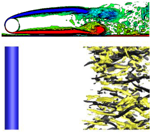
Figure 4 presents an overview of the ωx patterns for the cases with various Re and G/D combinations. Based on an examination of all the cases considered in this study (including those omitted in figure 4 due to space limit), it is found that beyond the complex wake transition regimes, the turbulent wakes of Re ≥ 300 are always dominated by small-scale rib-like mode B structures. With the increase in Re from 300 to 1000, the mode B structures gradually become increasingly chaotic (figure 4), which signifies increasingly turbulent wakes. On the other hand, the mode B structures are not noticeably influenced by G/D. The existence of solely mode B at Re ≥ 300 suggests that the flow and hydrodynamic characteristics (to be examined in §§ 3.2 and 3.3) may not experience sudden discontinuous changes in the present (Re, G/D) parameter space.

Figure 4. Instantaneous streamwise vorticity (ωx) fields for the cases with various Re and G/D combinations. The isosurfaces are ωx = ±1.5 for Re = 300 and ωx = ±5 for Re = 1000. Dark grey and light yellow denote positive and negative vorticity values, respectively. The flow is from left to right past the cylinder on the left. Although the cases with Re = 300 are simulated with Lz/D = 12, the ωx fields are shown with z/D = 0–6 so as to save space.
Figure 5 presents an overview of the vortex shedding (ωz) patterns for the cases with various Re and G/D combinations. For each case, the ωz field is shown at a phase when a lower (positive) vortex has just shed from the lower separating shear layer. Overall, alternate vortex shedding is observed for all the cases examined in this study (including those omitted in figure 5 due to space limits). With the increase in Re from 300 to 1000, both the streamwise vortices (figure 4) and spanwise vortices (figure 5) become increasingly chaotic. With the decrease in G/D, the vortex shedding (ωz) patterns are increasingly affected by the plane boundary. For G/D ≥ 0.3 (figure 5e–l), alternate roll up and shedding of the vortices can be clearly observed in each and every vortex shedding period. For G/D = 0.2, alternate roll up and shedding of the vortices can be observed over the majority (approximately two thirds) of the vortex shedding periods (e.g. figure 5c,d), but within some vortex shedding periods the lower separating shear layer hardly rolls up, and under such circumstance a very weak lower (positive) vortex is shed directly from the lower separating shear layer (e.g. figure 5a,b). In between of the neighbouring lower vortices, the upper (negative) vortices shed from the cylinder induce shear layers on the plane boundary with positive sign of vorticity. The newly shed weak lower vortex is then quickly annihilated or merged into the shear layers developed on the plane boundary with the same sign of vorticity. Strictly speaking, for G/D = 0.2 alternate vortex shedding (either with or without rolling up of the lower separating shear layer) still occurs for each and every vortex shedding period. However, without detailed numerical flow visualisation to capture the short-lived weak lower vortices, the shedding pattern may easily be classified as intermittent shedding from the lower separating shear layer. In any sense, at G/D = 0.2 the plane boundary alters the vortex shedding pattern.

Figure 5. Instantaneous spanwise vorticity (ωz) fields for the cases with various Re and G/D combinations. Each ωz field is obtained from the corresponding span-averaged flow field and is shown at a phase when a lower (positive) vortex has just shed from the lower separating shear layer. The contours of ωz are from −3 to 3, except for panels (b) and (d), where the contours are from −5 to 5.
In contrast to the scenario of flow past a cylinder in proximity to a stationary wall, where the intermediate range of G/D may be divided into several flow regimes with different types of interactions between the wall boundary layer and the lower shear layer generated by the cylinder (Price et al. Reference Price, Sumner, Smith, Leong and Païdoussis2002; He et al. Reference He, Wang, Pan, Feng, Gao and Rinoshika2017), the present results of a moving wall suggest that, without (i) the upstream wall boundary layer generated by a stationary wall, and (ii) very large velocity gradients towards the stationary wall (with ux = 0 on the wall), the vortex shedding pattern for G/D ≥ 0.3 remains very similar. Although shear layers also develop on a moving wall (as a result of the variation in the streamwise velocity in accordance with the propagation of shed vortices along the wake), these shear layers are much weaker than those generated on a stationary wall and thus do not alter the overall vortex shedding pattern.
At relatively small G/D, specifically smaller than a critical G/D within 0.2–0.5, the stationary wall suppresses the lower row of vortices (Bearman & Zdravkovich Reference Bearman and Zdravkovich1978; Price et al. Reference Price, Sumner, Smith, Leong and Païdoussis2002; Wang & Tan Reference Wang and Tan2008; Lin et al. Reference Lin, Lin, Hsieh and Dey2009; He et al. Reference He, Wang, Pan, Feng, Gao and Rinoshika2017). However, the present results of a moving wall show that the lower row of vortices still exists at G/D = 0.2. This difference suggests that for the scenario of a stationary wall, the lower row of vortices is largely suppressed by the development of the upstream wall boundary layer (rather than the near-wall effect). This finding may explain why different studies for the scenario of a stationary wall (by using different upstream wall boundary layers) obtained different critical G/D values for the suppression of alternate vortex shedding (generally between 0.2 and 0.5).
3.2. Time-averaged flow characteristics
As shown in figure 5, the streamwise location for the roll up and shedding of the spanwise vortices (and consequently the streamwise location for the development of the streamwise vortices shown in figure 4) depends strongly on both Re and G/D. This feature can be visualised and quantified more clearly by the streamlines obtained from the time- and span-averaged flow (figure 6), where the wake stagnation point (sketched in figure 7) provides an approximation of the streamwise location for the vortex shedding. By defining the wake recirculation length Lr as the streamwise distance from the centre of the cylinder to the wake stagnation point (figure 7), figure 8(a) summarises the Lr values for the cases with various Re and G/D combinations. In general, for each Re the Lr value reaches to a local minimum at G/D ~ 0.8, while for each G/D the Lr value increases with increasing Re. The increase in Lr with increasing Re was also observed by Noca, Park & Gharib (Reference Noca, Park and Gharib1998) for an unbounded cylinder (i.e. G/D → ∞). The consistent trend for the unbounded and near-wall scenarios suggests that the physical mechanism proposed for the unbounded scenario (Norberg Reference Norberg2003) may be applicable to the near-wall scenario. For an unbounded cylinder, Norberg (Reference Norberg2003) suggested that ‘the increase in secondary (essentially streamwise) circulation occurs probably at the expense of the primary (essentially spanwise) circulation associated with the roll-up of the von Kármán vortices’. With the increase in Re from 300 to 1000, the increase in the streamwise circulation is expected, as the wake becomes increasingly turbulent (shown by the increasingly chaotic mode B structures in figure 4), while the reduction in the spanwise circulation is examined as follows. In the present study, we quantify the mean spanwise circulation ( $\varGamma_z$) past x/D = 0.25 (i.e. feeding into the wake) per unit time. The mean circulation is obtained based on the time- and span-averaged flow field and is averaged between the upper and lower shear layers. The reason for the choice of x/D = 0.25 is that, at this point the shear layers have separated from the cylinder (such that there is no further accumulation of the circulation on the boundary layer), while the turbulence in the shear layer and wake (which may contribute undesirably to the sum of the circulation) have not yet developed. The $\varGamma_z$ value is calculated as
 \begin{equation}{\varGamma _z} = \frac{1}{2}\left( {\int_{upper\;shear\;layer} {\frac{{{u_x}}}{U}\textrm{|}{\omega_z}\textrm{|}\,\textrm{d}\left( {\frac{y}{D}} \right)} + \int_{lower\;shear\;layer} {\frac{{{u_x}}}{U}|{\omega_z}|\,\textrm{d}\left( {\frac{y}{D}} \right)} } \right)\!.\end{equation}
Figure 8(b) shows the variation of  $\varGamma_z$ with Re and G/D, which confirms that the spanwise circulation reduces with increasing Re from 300 to 1000, and thus explains the increase in Lr with increasing Re. Figure 8(b) also shows that for each Re, the spanwise circulation peaks at G/D ~ 0.6–0.8, which explains the local minimum in Lr at G/D around 0.8. The maximum spanwise circulation at G/D ~ 0.6–0.8 is physically linked to an increase in ux around the cylinder at intermediate G/D due to blockage effects, and a decrease in ux around the cylinder at small G/D due to flow deflection to the upper side of the cylinder. In figure 8(c), the ux around the cylinder is quantified by the mean ux sampled at x = 0 and within 1D both above and below the cylinder. Figure 8(c) confirms that the variation trend of this quantity resembles that of $\varGamma_z$. The quantitative differences between the variation trends shown in figure 8(b,c) is because the ux around the cylinder also influences the ωz around the cylinder, and they collectively shape the $\varGamma_z$ value through (3.3).

Figure 6. Streamlines of the time- and span-averaged flows for the cases with various Re and G/D combinations.

Figure 7. Definitions of the front stagnation point θf, upper separation angle θs 1, lower separation angle θs 2, upper bubble location Lb 1, lower bubble location Lb 2 and wake recirculation length Lr, illustrated based on the case (Re, G/D) = (300, 0.4). The blue curves represent streamlines of the time- and span-averaged flow, where two recirculation bubbles are observed behind the cylinder.

Figure 8. Wake characteristics for flow past a circular cylinder in proximity to a moving wall, quantified by (a) the wake recirculation length Lr/D, (b) the mean spanwise circulation  $\varGamma_z$ past x/D = 0.25, and (c) the mean streamwise velocity sampled at x = 0 and within 1D both above and below the cylinder.
The moving wall near the cylinder induces asymmetry of the flow about the wake centreline. The flow asymmetry is indicated by, for example, the non-zero streamwise distance between the upper and lower bubble locations (Lb 1–Lb 2)/D (figure 9a), the front stagnation point θf away from 0° (figure 9b) and different upper and lower separation angles (figure 9c,d). The definitions of these quantities are sketched in figure 7. Farther downstream, the flow asymmetry can be seen from the inclined streamlines shown in figure 6 (except for G/D = 3, where the flow asymmetry is negligible). Naturally, the level of flow asymmetry increases with decreasing G/D. It is also seen in figure 9(b–d) that θf is insensitive to the variation in Re, whereas θs 1 and θs 2 vary with both Re and G/D. This difference stems from the condition of an unbounded cylinder, where θf remains at 0° for all Re values, whereas θs 1 and θs 2 vary with Re. The flow asymmetry can also be reflected by (and can explain) some of the hydrodynamic characteristics examined in § 3.3.

Figure 9. Flow asymmetry about the wake centreline, quantified by (a) the streamwise distance between the upper and lower bubble locations (Lb 1–Lb 2)/D, (b) the front stagnation point θf, (c) the upper separation angle θs 1 and (d) the lower separation angle θs 2.
3.3. Hydrodynamic characteristics
Figure 10 summarises the hydrodynamic characteristics for the cases with various Re and G/D combinations. The close agreement between the results of G/D = 3 and 30 suggests that the effect of G/D becomes negligible at G/D  $\gtrsim $ 3. Below which, both G/D and Re may influence the hydrodynamic characteristics strongly.

Figure 10. Hydrodynamic characteristics for flow past a circular cylinder in proximity to a moving wall, quantified by (a) the time-averaged drag coefficient  $\overline {{C_D}}$, (b) the root-mean-square lift coefficient ${C^{\prime}_L}$, (c) the time-averaged lift coefficient $\overline {{C_L}}$ and (d) the Strouhal number St. For the majority of the cases, the St value is obtained via the CL signal, whereas for the cases (Re, G/D) = (600, 0.2), (800, 0.2), (1000, 0.2), (800, 0.3) and (1000, 0.3), the St value is obtained via the uy signal, and the results are distinguished by the dashed lines.
Specifically, the variation trends of  $\overline {{C_D}}$ (figure 10a) and ${C^{\prime}_L}$ (figure 10b) are generally consistent with that for $\varGamma_z$ (figure 8b) and inversely correlated with that for Lr (figure 8a). The reduction in $\varGamma_z$ and correspondingly the increase in Lr indicate downstream movement of the location for the vortex shedding, such that the alternate generation of the low-pressure regions at the locations of the vortex cores exerts less contribution to the mean suction and fluctuating lift back on the cylinder. However, while Lr increases significantly at G/D $\lesssim$ 0.4 (figure 8a), its effect on the reduction in $\overline {{C_D}}$ and ${C^{\prime}_L}$ seems less significant (figure 10a,b). This is because (i) the influence of the low pressure regions on the hydrodynamic forces is nonlinear (e.g. for Lr/D $\gtrsim $ 3–4 the ${C^{\prime}_L}$ value approaches zero already), and (ii) unlike the ${C^{\prime}_L}$ value which is solely induced by the alternate generation of the low pressure regions in the near wake, the $\overline {{C_D}}$ value is also significantly contributed by the positive pressure force on the front side of the cylinder (such that for Lr/D $\gtrsim $ 3–4, $\overline {{C_D}}$ does not approach zero).
Figure 10(c) shows the variation trend of  $\overline {{C_L}}$, which resembles the variation trend of θf (figure 9b). With the downward movement of the front stagnation point, a net lift is expected.
Figure 10(d) shows the variation of St with Re and G/D. The St value stays at a similar level (within 0.20–0.22) for G/D ≥ 0.4, but drops drastically with decreasing G/D below 0.4. An exception is observed for the case (Re, G/D) = (1000, 0.2), where St remains at around 0.20 (to be closely examined later on). Figure 10(d) also shows the variation of St with G/D for the scenario of a stationary wall obtained experimentally by Lin et al. (Reference Lin, Lin, Hsieh and Dey2009), He et al. (Reference He, Wang, Pan, Feng, Gao and Rinoshika2017) and Li et al. (Reference Li, Wang, Qiu, Wu, Zhou, Fu and Liu2022). Their results indicate that St increases significantly as G/D decreases from approximately 2 to 0.5, but decreases with further decrease in G/D. A comparison between the stationary and moving wall results suggests that the increase in St over G/D ~ 2–0.5 for a stationary wall is attributed to the development of the upstream wall boundary layer, whereas the drastic reduction in St at G/D  $\lesssim$ 0.4 is due to the near-wall effect.
3.4. Frequency spectra of lift and velocity signals
The cases with Re = 1000 and different G/D values are used to further illustrate the characteristics of the vortex shedding frequency. Figure 11 shows the frequency spectra of the lift signal (CL) sampled at the location of the cylinder (i.e. at x ~ 0), while figure 12 shows the frequency spectra of the transverse velocity signal (uy) sampled at a location closer to the streamwise location of vortex shedding. This location is chosen at x/D = Lr/D − 1 and y/D = 0.5, and eight equally spaced spanwise locations are used to average the frequency spectrum. Figures 11(a) and 12(a) show the frequency spectra of CL and uy in linear scales, which reveal clearly the broad-bandedness and strength of the dominant frequencies. Figures 11(b) and 12(b) show the power spectra of CL and uy in logarithmic scales, where EL and Euy are calculated as
 \begin{gather}\int_0^\infty {{E_L}\,\textrm{d}\left( {\frac{f}{{{f_L}}}} \right)} = C^{\prime 2}_L,\end{gather}
 \begin{gather}\int_0^\infty {{E_{uy}}\,\textrm{d}\left( {\frac{f}{{{f_{uy}}}}} \right)} = \frac{{\overline {{u^{\prime}_y}{u^{\prime}_y}} }}{{{U^2}}}.\end{gather}
The logarithmic scales may help reveal very weak frequencies which are difficult to be identified in linear scales.

Figure 11. Frequency spectra of CL for the cases with Re = 1000 and various G/D values: (a) frequency spectra of CL in linear scales; (b) power spectra of CL in logarithmic scales, where each spectrum (other than the top one) is shifted downward by three orders of magnitude.

Figure 12. Frequency spectra of uy sampled at a location close to the streamwise location of vortex shedding (i.e. x/D = Lr/D − 1 and y/D = 0.5) for the cases with Re = 1000 and various G/D values: (a) frequency spectra of uy in linear scales; (b) power spectra of uy in logarithmic scales, where each spectrum (other than the top one) is shifted downward by three orders of magnitude.
For the present cases with various Re and G/D combinations, a common finding is that, for the cases with vortex shedding occurring relatively far from the cylinder (specifically with Lr/D > 6.7, see figure 8a), the St value can hardly be identified from the frequency spectra of CL. For example, figure 11(a) shows the frequency spectra of CL for the cases with Re = 1000 and various G/D, where the frequency peak becomes absent for G/D ≤ 0.3 (such that the noise level at fL ~ 0, which is always of the order of magnitude of 10−3 for different G/D, becomes dominant).
With the aid of the logarithmic scales in figure 11(b), very weak vortex shedding frequency peaks may be observed for G/D = 0.3 and 0.2. Nevertheless, it is difficult to identify a definite St value, because there exists a broad-band region of frequencies without a dominant frequency peak (and the dominant frequency fL required for plotting figure 11b is actually borrowed from fuy identified in figure 12a), and the broad-band frequencies are only marginally above the noise level.
To obtain the dominant St values for G/D = 0.3 and 0.2, we instead use the uy signals sampled at a location closer to the streamwise location of vortex shedding (i.e. x/D = Lr/D − 1 and y/D = 0.5). The St values obtained from the uy signals are shown in figure 10(d) with dashed lines, and examples of frequency spectra of uy for the cases with Re = 1000 are shown in figure 12. The case G/D = 0.4 confirms that the frequency spectra of CL and uy yield identical St, and flow visualisation of this case confirms that the time period for each vortex shedding cycle is indeed approximately 1/St. For G/D = 0.3 and 0.2, the St values can hardly be determined from the CL signal (figure 11), but can be revealed by a uy signal sampled close to the location of vortex shedding (figure 12). The existence of a frequency peak in the uy spectrum is consistent with the observation of clear vortex shedding from flow visualisation (figure 5). Based on flow visualisation, it is also found that the time periods for different vortex shedding cycles may vary noticeably. The noticeable variation in the vortex shedding period is attributed to the time variation in strength of the positive vortices shed from the lower side of the cylinder (reflected by different degrees of rolling up before shedding) due to the near-wall effect. Consequently, the uy spectra for G/D = 0.3 and 0.2 (figure 12a) are relatively broad-band. For G/D = 0.2, the frequency peak is only slightly larger than the amplitudes of a range of other frequencies, which partly explains why the St value for this case deviates from the general trend (figure 10d). For this case, the St value simply corresponds to a vortex shedding frequency that is slightly more dominant than others, but a range of other frequencies are also observed in figure 12(a).
Another key finding is that, a negligible frequency peak with no dominant St value in the CL spectrum does not necessarily indicate absence of, or negligible, vortex shedding phenomenon. The use of a readily available CL spectrum as the criterion for the determination of the critical G/D for the suppression of vortex shedding (as was used by several previous studies for the case of a stationary wall) may lead to inaccurate conclusion.
3.5. Turbulent kinetic energy
This section examines the influence of Re and G/D on the mean TKE in the wake region. At each spatial location, the TKE is calculated as  $(\overline {{u^{\prime}_x}{u^{\prime}_x}} + \overline {{u^{\prime}_y}{u^{\prime}_y}} + \overline {{u^{\prime}_z}{u^{\prime}_z}} )/(2{U^2})$, where ${u^{\prime}_i} = {u_i} - \overline {{u_i}}$. Figure 13 illustrates the velocity variance fields for the cases with various Re and G/D combinations. The velocity variance patterns are significantly affected by G/D and relatively less affected by Re. For G/D = 3, the velocity variance patterns are largely symmetric about the wake centreline, whereas for G/D = 0.2, the patterns are significantly altered. Since different cases may display very different velocity variance patterns, it is less meaningful to simply compare the peak value or any specific spatial location. In the present study, the TKE (and its three components) of different cases are compared after integrating the result along the y-direction, i.e.
 \begin{gather}{e_x} = \frac{1}{2}\int {\frac{{\overline {{u^{\prime}_x}{u^{\prime}_x}} }}{{{U^2}}}} \,\textrm{d}\left( {\frac{y}{D}} \right)\!,\end{gather}
 \begin{gather}{e_y} = \frac{1}{2}\int {\frac{{\overline {{u^{\prime}_y}{u^{\prime}_y}} }}{{{U^2}}}} \,\textrm{d}\left( {\frac{y}{D}} \right)\!,\end{gather}
 \begin{gather}{e_z} = \frac{1}{2}\int {\frac{{\overline {{u^{\prime}_z}{u^{\prime}_z}} }}{{{U^2}}}} \,\textrm{d}\left( {\frac{y}{D}} \right)\!.\end{gather}
Figure 13. Velocity fluctuation fields for the cases with various Re and G/D combinations. In each panel, the contours are from 0 to the maximum value with 20 equal intervals. The velocity components are normalised by U already.
Figure 14 shows the integrated kinetic energy components for the cases with Re = 1000 and various G/D values. For each case, the relative strengths of the three energy components generally follow ey > ex > ez. The anisotropy of the kinetic energy in the wake is largely due to the contribution of the primary vortices to ey and ex. For example, Jiang et al. (Reference Jiang, Hu, Cheng and Zhou2022) investigated the case of an unbounded cylinder (i.e. G/D → ∞) at Re = 1000 and examined the anisotropy of the kinetic energy at x/D = 10 and 20 and found that, by removing the contribution of the primary vortices, the kinetic energy became much more isotropic. For the present cases with different G/D, the maximum ez value stays consistently at ~0.04–0.05 (since ez is not directly contributed by the primary vortices), whereas the maximum ex and ey values (highlighted by dots in figure 14a,b) vary with G/D, which suggests that for different G/D the contribution from the primary vortices may be different.

Figure 14. Integrated kinetic energy components for the cases with Re = 1000 and various G/D values: (a) the ex component; (b) the ey component; (c) the ez component; (d) the sum of three components.
For the cases with various Re and G/D combinations, the magnitude and streamwise location for the maximum ey values (denoted ey,max) are plotted in figure 15. Although the kinetic energy in the wake is not solely contributed by this maximum value, it serves as a crude indication of the variation of the kinetic energy with the characteristics of the primary vortices. Specifically, the variation of ey,max (figure 15a) resembles that of  $\varGamma_z$ (figure 8b), while the variation of the streamwise location of ey,max (figure 15b) resembles that of Lr (figure 8a). These resemblances suggest that the strength and streamwise location of the shed primary vortices dictate the point of ey,max and thus influence strongly the kinetic energy in the wake.

Figure 15. Characteristics of the maximum ey for the cases with various Re and G/D combinations: (a) the magnitude, and (b) the streamwise location (with a resolution of Δx/D = 0.2).
Figure 16 shows the variation of the total TKE (E) in the wake region (per unit span length) with Re and G/D, where E is calculated as
 \begin{equation}E = \int {({e_x} + {e_y} + {e_z})\,\textrm{d}\left( {\frac{x}{D}} \right)} .\end{equation}
Two different wake regions are considered, i.e. x/D = 0–15 (figure 16a) and x/D = 0–30 (figure 16b). Their similarity suggests that the variation trends are not significantly affected by the choice of the streamwise range. A major feature shown in figure 16 is that E reduces drastically as G/D reduces below 0.8. As discussed with the aid of ey,max, the reduction of E is due to both (i) reduction in the strength of the shed vortices and (ii) downstream movement of the location of vortex shedding. In addition, with the downstream movement of the primary vortices, the streamwise vortices are also generated farther downstream (cf. figures 4 and 5), which leads to a delayed growth of ez (figure 14c). The above-mentioned three factors contribute collectively to the significant reduction of E shown in figure 16.

Figure 16. Variation of the total TKE in the wake region with Re and G/D: (a) over the wake region of x/D = 0–15, and (b) over the wake region of x/D = 0–30.
4. Conclusions
This study examines the scenario of flow past a circular cylinder in proximity to a moving wall (or equally a body translating in still fluid parallel to a stationary wall) over the parameter space of Re = 300–1000 and G/D = 0.2–3. Visualisation of the streamwise vortices shows that the turbulent wakes of Re ≥ 300 (beyond the wake transition regimes) are always dominated by small-scale rib-like mode B structures which gradually become increasingly chaotic with increasing Re. Visualisation of the spanwise vortices shows that alternate vortex shedding persists for all cases. The only distinctive feature is that, for G/D = 0.2 the shedding of the lower (positive) vortices may be relatively weak – for approximately one third of the vortex shedding periods the lower vortices are shed without rolling up of the separating shear layer.
Over the (Re, G/D) parameter space, the variations in the flow, hydrodynamic and turbulence characteristics and their underlying physical mechanisms are examined in detail. The major findings are summarised below.
(i) Flow characteristics. The streamwise location for the vortex shedding (quantified by Lr) depends strongly on both Re and G/D. In general, for each Re the Lr value reaches to a local minimum at G/D ~ 0.8, while for each G/D the Lr value increases with increasing Re. The variation of Lr with Re and G/D can be explained by the spanwise circulation $\varGamma_z$ fed into the wake, where the variation trend of Lr is inversely correlated with that of $\varGamma_z$. The local maximum of $\varGamma_z$ at G/D ~ 0.6–0.8 is physically linked to an increase in the streamwise velocity around the cylinder at intermediate G/D due to blockage effect, while the reduction in $\varGamma_z$ with increasing Re is because the streamwise circulation draws increasing energy from the spanwise circulation.
(i) Hydrodynamic characteristics. The variation trends of the hydrodynamic coefficients
$\overline {{C_D}}$ and ${C^{\prime}_L}$ are generally consistent with that of $\varGamma_z$ and inversely correlated with that of Lr. Physically, when the location of vortex shedding moves downstream, the alternate generation of the low-pressure regions at the locations of the vortex cores exerts less contribution to the mean suction and fluctuating lift back on the cylinder. The variation trend of $\overline {{C_L}}$ is consistent with that of the front stagnation point θf. Physically, with the downward movement of the front stagnation point, a net lift is expected.(iii) Turbulence characteristics. The total kinetic energy in the wake region reduces drastically as G/D reduces below 0.8. The reduction of E is contributed collectively by (i) reduction in the strength of the shed vortices, (ii) downstream movement of the location of vortex shedding and (iii) downstream movement of the location of the streamwise vortices associated with the delayed generation of primary vortices.


The present results on a moving wall also help to explain several flow and hydrodynamic characteristics reported in the literature for a stationary wall. For example, the existence of alternate vortex shedding for a moving wall at G/D = 0.2 suggests that the suppression of the lower row of vortices for a stationary wall at G/D = 0.2–0.5 is due to the development of the upstream wall boundary layer (rather than the near-wall effect), and different wall boundary layers may result in different critical G/D values between 0.2 and 0.5. A comparison between the stationary and moving wall results also suggests that, the increase in St over G/D ~ 2–0.5 for a stationary wall is attributed to the development of the upstream wall boundary layer, whereas the drastic reduction in St at G/D  $\lesssim$ 0.4 is attributed to the near-wall effect.
Funding
H.J. would like to acknowledge support from the National Natural Science Foundation of China (grant no. 52301341).
Declaration of interests
The authors report no conflict of interest.


 Open access