


1. Introduction
Accurate prediction of the separation pattern at a stall condition is crucial in ensuring the safety of aircraft because the separation causes loss of local lift, which potentially induces harmful pitch-up motion. One of the typical separation patterns on aircraft is corner-flow separation at the wing–body junction. Near the junction, the boundary layers over the wing and fuselage interact, causing a low-velocity region prone to separation. Therefore, substantial efforts have been made to understand and predict wing–body juncture flows, as summarized by Gand et al. (Reference Gand, Deck, Brunet and Sagaut2010). More recently, the NASA Juncture Flow experiment (Rumsey, Neuhart & Kegerise Reference Rumsey, Neuhart and Kegerise2016; Rumsey et al. Reference Rumsey, Ahmad, Carlson, Kegerise, Neuhart, Hannon, Jenkins, Yao, Balakumar and Gildersleeve2022) was conducted to obtain validation data for computational simulations. They employed a simplified wing–body geometry, and measured velocity and Reynolds stress profiles in the corner region by laser Doppler velocimetry. Subsequent studies (Abe, Mizobuchi & Matsuo Reference Abe, Mizobuchi and Matsuo2020; Abdol-Hamid et al. Reference Abdol-Hamid, Ahmad, Carlson and Biedron2020; Eisfeld et al. Reference Eisfeld, Rumsey, Togiti, Braun and Stürmer2022; Ghate et al. Reference Ghate, Housman, Stich, Kenway and Kiris2020; Iyer & Malik Reference Iyer and Malik2020; Lozano-Duran, Bose & Moin Reference Lozano-Duran, Bose and Moin2020; Rumsey et al. Reference Rumsey, Carlson, Pulliam and Spalart2020) have utilized the data from this experiment to validate and improve simulation methodologies and turbulence models.
One of the crucial features of wing-body juncture flows is the interaction between the boundary layers over the wing and body. The side-wall interaction causes the second type of Prandtl's secondary flow (Bradshaw Reference Bradshaw1987), i.e. a flow motion caused by the anisotropy of the Reynolds normal stress. The secondary flow motion appears as a pair of longitudinal (i.e. streamwise) vortices at the corner. A typical example of this type of flow is the flow in a square duct, which has been investigated by many researchers (e.g. Pinelli et al. Reference Pinelli, Uhlmann, Sekimoto and Kawahara2010; Vinuesa et al. Reference Vinuesa, Noorani, Lozano-Durán, El Khoury, Schlatter, Fischer and Nagib2014; Zhang et al. Reference Zhang, Trias, Gorobets, Tan and Oliva2015; Pirozzoli et al. Reference Pirozzoli, Modesti, Orlandi and Grasso2018). Most recently, Pirozzoli et al. (Reference Pirozzoli, Modesti, Orlandi and Grasso2018) conducted direct numerical simulations (DNS) of square duct flows at several Reynolds numbers up to the friction Reynolds number  $Re_\tau =1.0\times 10^3$, and discussed the transport of velocity and vorticity. They showed that the secondary motion transports streamwise momentum towards the duct corner. Hence the secondary motion essentially delays the corner-flow separation. However, the effects of the secondary vortices on the corner-flow separation have rarely been discussed quantitatively in previous studies. The challenges to this kind of discussion are that square duct flows do not involve corner-flow separation, whereas realistic wing–body juncture flows are too complex for quantitative analysis of the momentum transport by the secondary motion.
Moreover, simulating corner-flow separation using turbulence models based on the Reynolds-averaged Navier–Stokes (RANS) equations also poses challenges. In particular, the turbulence model must reproduce accurately the anisotropy of Reynolds stress, which cannot be realized by classical turbulence models based on the Boussinesq approximation. Hence several types of turbulence models have been proposed to incorporate the effects of anisotropy. One approach is the Reynolds stress transport models (e.g. Launder, Reece & Rodi Reference Launder, Reece and Rodi1975; Speziale, Sarkar & Gatski Reference Speziale, Sarkar and Gatski1991), which involve six partial differential equations to account for the six independent components of Reynolds stress. To reduce computational costs, several researchers (e.g. Gatski & Speziale Reference Gatski and Speziale1993; Wallin & Johansson Reference Wallin and Johansson2000) have also proposed algebraic stress models. In these models, the Reynolds stress equations are reduced to algebraic equations. Another approach, which is simpler than the models above, is the model based on the nonlinear expression of Reynolds stress (e.g. Speziale Reference Speziale1987; Spalart Reference Spalart2000). One of the most prevalent models in this approach is the quadratic constitutive relation (QCR) proposed by Spalart (Reference Spalart2000) (often referred to as QCR2000). This model provides each Reynolds stress component by a simple algebraic equation consisting only of scalar eddy viscosity, strain, vorticity, and one constant parameter. More recently, modifications to QCR2000 have also been proposed (Mani et al. Reference Mani, Babcock, Winkler and Spalart2013; Rumsey et al. Reference Rumsey, Carlson, Pulliam and Spalart2020). Mani et al. (Reference Mani, Babcock, Winkler and Spalart2013) introduced a modification to QCR2000 that incorporates the effects of turbulence kinetic energy, which are not included in the original Spalart–Allmaras (SA) turbulence model. Additionally, Rumsey et al. (Reference Rumsey, Carlson, Pulliam and Spalart2020) investigated the validity of the QCR based on data from the NASA Juncture Flow experiment, and presented a modified version of the model where the model parameters vary in space.
Several existing studies have reported that the QCR improves the prediction of the corner-flow separation at the wing–body junction. Yamamoto, Tanaka & Murayama (Reference Yamamoto, Tanaka and Murayama2012) found that the SA turbulence model with QCR2000 shows the pitch-up motion of the DLR-F6 aircraft model at the high angle of attack. This trend is in good agreement with the past wind tunnel experiment (Rivers & Dittberner Reference Rivers and Dittberner2011), while the baseline SA model (without QCR2000) does not predict it. The remarkable difference between the two simulation results is the side–body separation (i.e. the corner-flow separation at the wing–body junction). Here, QCR2000 suppresses the side–body separation, resulting in the correct pitch motion at high angles of attack. Yamamoto et al. (Reference Yamamoto, Tanaka and Murayama2012) explained that the difference in the side–body separation occurs because the secondary motion convects momentum to the corner region. Dandois (Reference Dandois2014) also reported a similar improvement in predicting the corner-flow separation of the DLR-F6 aircraft model. After these studies, QCR2000 has been used widely in RANS simulations of aircraft at high angles of attack (e.g. Rumsey Reference Rumsey2018; Tamaki & Imamura Reference Tamaki and Imamura2018; Tinoco et al. Reference Tinoco2018).
However, despite the prevalence of the model, the validity of the parameter of QCR2000 (referred to as  $C_{cr1}$ in the original paper) remains unclear. Spalart (Reference Spalart2000) showed qualitative improvement in predicting the secondary motion of a square duct flow compared to the baseline turbulence model using the Boussinesq approximation. The square duct flow and the wing–body junction flow differ in many points, such as the existence of the corner-flow separation or the streamwise development of the boundary layer. Furthermore, although modifications to QCR2000 (Mani et al. Reference Mani, Babcock, Winkler and Spalart2013; Rumsey et al. Reference Rumsey, Carlson, Pulliam and Spalart2020) have been proposed, their validation has been limited to comparisons to the measurements in wind tunnel experiments. Therefore, comprehensive validation using a database from high Reynolds number DNS or large-eddy simulation (LES) will be beneficial for a better understanding and improvement of the QCR.
Considering the situations stated in the preceding paragraphs, we conduct a LES of a simplified side-wall interference flow field imitating the wing–body junction of aircraft. The purpose of this simulation is twofold. The first purpose is to explain the effects of the secondary motion on the corner-flow separation based on the momentum budget analysis. Unlike the former studies on square duct or wing–body junction flows, the geometry simulated in this study involves corner-flow separation while retaining a simple geometry suitable for the budget analysis. The second purpose is to provide databases for turbulence modelling. (The obtained data are uploaded on the website https://www.klab.mech.tohoku.ac.jp/database.) Using the obtained database, we investigate the validity of the constitutive relations and propose a QCR that can reproduce the Reynolds stress distributions better. Also, to eliminate undesirable low Reynolds number effects, we conduct the simulation at a relatively high Reynolds number  ${Re}_L\sim 10^6$, where ${Re}_L$ is the Reynolds number based on the freestream velocity and the length from the leading edge. This Reynolds number is comparable to that of large-scale wind tunnel testing. Pirozzoli et al. (Reference Pirozzoli, Modesti, Orlandi and Grasso2018) have reported in their study on the square duct flow that the strength of the secondary motion saturates at high Reynolds numbers. Since a LES at a high Reynolds number requires massive computational resources, the database may be obtained first by the state-of-the-art supercomputer.
The structure of this paper is as follows. In § 2, the computational setting and methodologies of the LES are presented. Then § 3 describes the results from the LES and analyses based on the momentum and vorticity budgets, which will explain the effects and generation mechanism of the secondary motion. In § 4, we explore the modelling of the constitutive relation using the LES data, and propose a modified QCR. The developed model is validated in RANS simulations in § 5, and finally, § 6 provides the concluding remarks.
2. LES computational set-up
2.1. Geometry
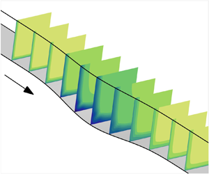
We simulate the side-wall interference flow field shown in figure 1. The computational domain has a square cross-section whose size increases and decreases in the streamwise direction. The boundary layers on the bottom and side walls interfere, and the change in the cross-section induces a pressure gradient in the streamwise direction. The shape of the walls is designed so that a small separation bubble occurs at the corner of the diverging and converging sections. Here, the bottom wall coordinate  $y_w$ is defined as
 \begin{equation} y_w=\left\{\begin{array}{@{}ll} y_0 & \left(0\leqslant x/L<1.0\ {\rm and}\ x/L>2.0\right),\\ y_0-H\sin^4({\rm \pi} (x-x_0)/W) & \left(1.0\leqslant x/L\leqslant2.0\right), \end{array}\right. \end{equation}
where  $y_0=-0.16L$, $H=0.03L$, $x_0=W=L$ (see figure 2a), and $L$ is the length between the leading edge and the starting position of the change in the wall geometry. These parameters were determined through preliminary RANS analysis so that corner-flow separation occurs while the boundary layer away from the side wall does not separate. The wall starts from $x=0$, and the laminar boundary layer is tripped at $x/L=0.1$ by introducing the unsteady body force presented by Schlatter & Örlü (Reference Schlatter and Örlü2012). The parameters for the tripping, such as the temporal and spatial cut-off scales, are the same as the baseline case in Schlatter & Örlü (Reference Schlatter and Örlü2012), where we employ the laminar displacement thickness at the tripping location $\delta ^*_0/L=6.0\times 10^{-4}$. The side wall is set so that the geometry is symmetric about $y=z$. Also, a periodic boundary condition is implemented so that velocity vector $(u,v,w)$ and pressure $p$ at $y/L=0$ match $(u,-w,v)$ and $p$ at $z/L=0$, respectively. The Reynolds number based on the freestream velocity $u_\infty$ and length $L$, i.e. $Re_L\equiv u_\infty L/\nu _\infty$, is set to $1.0\times 10^6$, where $\nu _\infty$ is the freestream kinematic viscosity. At $x/L=1.0$, the Reynolds number $Re_L=1.0\times 10^6$ corresponds to $Re_\theta \equiv u_\infty \theta /\nu _\infty \approx 2.0\times 10^3$ and $Re_\tau \equiv u_\tau \delta _{99} /\nu _w \approx 6.9\times 10^2$, where $\theta$ is the momentum thickness, $\delta _{99}$ is the 99 % boundary layer thickness, $u_\tau$ is the friction velocity, and $\nu _w$ is the kinematic viscosity at the wall.

Figure 1. Geometry of the side wall interference flow field.

Figure 2. The LES computational grid: (a)  $x$–
$x$– $z$ plane at $y/L=0.0$ (every 50 grid points are shown); (b) $y$–
$y$– $z$ planes (every 20 grid points are shown).
2.2. Computational grid
The computational grid is a structured curvilinear grid. As shown in figure 2, the grid within the  $y$–
$y$– $z$ plane is orthogonal, while the streamwise grid lines are not always perpendicular to the $y$–
$y$– $z$ plane. In the turbulent flow region ( $x/L>0.1$), the grid spacing in the streamwise direction is set to $3.0\times 10^{-4}L$ to $4.0\times 10^{-4}L$. In $x/L<1.0$, the spanwise grid spacing, except for the near-wall region, is set to $2.0\times 10^{-4}L$. In the diverging and converging sections ( $1.0< x/L< 2.0$), the near-wall grid resolution is retained, while the outer grid in the $y$–
$y$– $z$ plane is stretched slightly as shown in figure 2(b). These grid spacings are determined based on the viscous wall unit at $(x/L,y/L)=(1.0,0.0)$, i.e. a zero-pressure gradient location sufficiently away from the side wall. At this location, the streamwise and spanwise grid spacings in the wall viscous unit are approximately 16 and 8, respectively. Also, the wall-normal grid spacing at the wall is $1.5\times 10^{-5}L$, which is determined so that the spacing in the wall viscous unit does not exceed 0.9. In the diverging and converging sections, the grid spacing in the wall viscous unit becomes less than that described above because the skin friction decreases.
2.3. Numerical methods
The present simulation is based on the spatially filtered compressible Navier–Stokes equations. The fluid is an ideal gas with molecular viscosity following Sutherland's law. Here, we employ an implicit LES regime that has been well validated in our previous works (e.g. Kawai, Shankar & Lele Reference Kawai, Shankar and Lele2010; Asada & Kawai Reference Asada and Kawai2018; Tamaki & Kawai Reference Tamaki and Kawai2023). The space is discretized based on the finite-difference method, where the spatial derivatives are evaluated by the sixth-order compact difference scheme (Lele Reference Lele1992). Also, we introduce the tridiagonal compact filter (Lele Reference Lele1992; Gaitonde & Visbal Reference Gaitonde and Visbal2000) to remove high-frequency numerical oscillations. Since the filter plays a similar role to a subgrid-scale (SGS) turbulence model, the simulation does not employ any explicit SGS turbulence model.
For the time integration, we employ a second-order implicit scheme (Obayashi, Fujii & Gavali Reference Obayashi, Fujii and Gavali1988; Izuka Reference Izuka2006) with five subiterations per time step. The magnitude of the residual reduces by more than two orders during the subiterations. Here, the time increment is set to  $\Delta t\, u_\infty /L=2.4\times 10^{-5}$, corresponding to a viscous-scale time increment $\Delta t^+\sim 0.1$ and maximum Courant number approximately 8. According to the previous studies (Choi & Moin Reference Choi and Moin1994; Kawai et al. Reference Kawai, Shankar and Lele2010), this time increment ( $\Delta t^+\sim 0.1$) is sufficiently small for simulating wall turbulence.
The present LES is conducted on the Fugaku supercomputer provided by the RIKEN Center of Computational Science. The computational domain is divided into  $60\times 8\times 8$ subdomains, where the message-passing interface is used for inter-subdomain communications. Here, four subdomains are allocated per computational node (48 cores A64FX CPU). Furthermore, the computation for each subdomain is parallelized by OpenMP with 12 threads.
2.4. Statistical averaging
For statistical averaging, we conduct the simulation during a period  $T_{ave}u_\infty /L=144$ ( $6\times 10^6$ time steps) after an initial period $Tu_\infty /L=33.6$, where $T$ is the time. Previous studies on square duct flows (Pinelli et al. Reference Pinelli, Uhlmann, Sekimoto and Kawahara2010; Vinuesa et al. Reference Vinuesa, Noorani, Lozano-Durán, El Khoury, Schlatter, Fischer and Nagib2014; Pirozzoli et al. Reference Pirozzoli, Modesti, Orlandi and Grasso2018) reported that the statistical convergence of the secondary flow motion takes far longer than the convective time unit. In these studies, the statistical average is taken for $T_{\rm ave} U_b/h$ from $5.9\times 10^3$ (Vinuesa et al. Reference Vinuesa, Noorani, Lozano-Durán, El Khoury, Schlatter, Fischer and Nagib2014) to $1.0\times 10^4$ (Pirozzoli et al. Reference Pirozzoli, Modesti, Orlandi and Grasso2018), where $U_b$ is the bulk velocity, and $h$ is the half-height of the duct. Since the present simulation consists of developing boundary layers, we use the nominal freestream velocity $u_\infty$ and the boundary layer thickness $x/L=1.0$ ( $\delta _{99}/L=0.0164$; see § 3.1) for the normalization. Essentially, these values have the same meaning as $U_b$ and $h$ in the duct-flow cases. The averaging period using these scales is calculated as $T_{ave} u_\infty /\delta _{99}=8.8\times 10^3$, which has the same order of magnitude as values in the studies described above.
Also, when showing cross-sectional distributions of variables, we take averaging through the range  $\pm 0.01L$ in the $x$ direction and by inverting around the $y=z$ line. Appendix A summarizes the statistical convergence and the effects of the spatial averaging.
3. LES results
3.1. Overview
To validate the employed methodologies and computational grid, we first examine the velocity and Reynolds stress profiles of the fully developed turbulent boundary layer at  $x/L=1.0$, where the pressure gradient is almost negligible. Here, the obtained data are averaged over $z/L\in [-0.01,0.0]$, which is sufficiently away from the side wall. At this location, $\delta _{99}/L=0.0169$ and $\theta /L=0.00204$ (i.e. $Re_\theta =2.04\times 10^3$). Figure 3 compares the obtained mean streamwise velocity and Reynolds stress profiles in the wall viscous units to the DNS data at a similar Reynolds number ( $Re_\theta =2.00\times 10^3$) presented by Schlatter & Örlü (Reference Schlatter and Örlü2010). Here, the overline and prime denote averaged and fluctuating components, respectively. In the results, both streamwise velocity and Reynolds stress components are in excellent agreement with the DNS data. These results show that the spatial and temporal resolutions of the present LES are sufficiently high as wall-resolved LES and closer to DNS. Note that the density fluctuation is less than $1\,\%$ of the freestream value, suggesting that the flow is almost incompressible.

Figure 3. Turbulence statistics at  $x/L=1.0$. Lines and symbols denote the present LES and DNS data by Schlatter & Örlü (Reference Schlatter and Örlü2010), respectively. (a) Streamwise velocity. (b) Reynolds stress.
Figure 4 shows the distributions of  $\bar {u}$, mean pressure coefficient $C_p$, and mean skin friction coefficient $C_f$ over the periodic boundary plane ( $y/L=0.0$). As shown here, the flow decelerates by the expansion of the cross-section in $1.0< x/L<1.5$, where an adverse pressure gradient occurs. Since the pressure gradient is mild, $C_f$ remains positive, i.e. the mean flow separation does not occur at the locations away from the side wall, though the flow involves the corner-flow separation as described in the following paragraph. Furthermore, $C_f$ in $x/L<1.0$ shows reasonable agreement with the classical power-law flat-plate correlation $C_f=0.027\,Re_x^{-1/7}$ (White Reference White2006), where $Re_x \equiv u_\infty x/\nu _\infty$.

Figure 4. Mean streamwise velocity, pressure coefficient and skin friction coefficient distributions over the periodic boundary plane ( $y/L=0$) obtained by the LES.
Next, we examine the entire flow field, including the effects of the side wall. Figure 5 shows the distributions of  $\bar {u}$, turbulence kinetic energy (TKE) $\bar {K}\equiv (\overline {u'u'}+ \overline {v'v'}+\overline {w'w'})/2$, and mean streamwise vorticity $\overline {\omega _x}\equiv \partial \bar {w}/\partial y - \partial \bar {v}/\partial z$ at several streamwise sections. The streamwise velocity distributions indicate that flow separation occurs at the corner near $x/L=1.4$ and reattaches at $x/L\approx 1.6$. In the diverging section ( $1.0< x/L<1.5$), the TKE distributions (see figure 5b) show a significant increase. Also, in figure 5(c), a vortex pair is observed at the corner of each section. The size of the vortices increases as the flow field diverges and is distributed away from the corner.

Figure 5. Overview of the statistically averaged flow field in the diverging and converging sections obtained by the LES: (a) mean streamwise velocity  $\bar {u}/u_\infty$; (b) TKE $\bar {K}/u_\infty ^2$; (c) mean streamwise vorticity $\bar {\omega }_x L/u_\infty$.
Figure 6 shows the mean velocity distributions near the corner at streamwise cross-sections  $x/L=1.0$, 1.5 and 2.0. The contours of the streamwise velocity bulge into the corner, which is especially remarkable at $x/L=1.5$. As will be indicated in § 3.2, this bulge occurs due to the momentum transport by the secondary motion and delays the corner-flow separation. Furthermore, the cross-sectional velocity contours show the secondary motion, i.e. a cross-plane flow occurs along the diagonal line toward the corner, and an outward flow occurs along the wall. At $x/L=1.0$, the secondary motion is similar to the DNS square duct case Pirozzoli et al. (Reference Pirozzoli, Modesti, Orlandi and Grasso2018). The maximum cross-sectional velocity in the $x/L=1.0$ plane is $0.017u_\infty$, which agrees with Pirozzoli et al. (Reference Pirozzoli, Modesti, Orlandi and Grasso2018), who reported that the maximum cross-sectional velocity is approximately 2 % of the duct centreline velocity. Also, figure 7 shows the distribution of $v$ at $x/L=1.0$ with axes in the wall viscous units. Note that these wall viscous units are calculated using $u_\tau$ at the centreline ( $y=0$). Pirozzoli et al. (Reference Pirozzoli, Modesti, Orlandi and Grasso2018) reported that the maximum cross-sectional velocity occurs at $y^+\approx 10$ and $50\lesssim z^+\lesssim 100$, where they used the span-averaged $u_\tau$ for calculating the wall viscous units. Although there are slight differences in the definition of $u_\tau$, the velocity distribution shown in figure 7 shows good agreement with their results. In the downstream ( $x/L=1.5$), the cross-sectional velocity is higher and more widely distributed than for $x/L=1.0$. At $x/L=2.0$, the secondary motion remains in a broader area compared to $x/L=1.0$, which shows the history of the divergence of the flow field geometry.

Figure 6. Mean velocity distributions over the streamwise cross-sections near the corner at (a,d)  $x/L=1.0$, (b,e) $x/L=1.5$ and (c,f) $x/L=2.0$, where $z_w$ is the coordinate of the side wall. In (d–f), negative contours are shown with black dashed lines (also applied to the following figures). Note that the scale of the in-plane velocity vectors varies with cross-section location. (a–c) Streamwise velocity $\bar {u}/u_\infty$. (d–f) Cross-sectional velocity $\bar {v}/u_\infty$ with in-plane velocity vectors.

Figure 7. Cross-sectional velocity  $\bar {v}/u_\infty$ near the corner at $x/L=1.0$ with axes in wall viscous units.
Figure 8 shows the distributions of the Reynolds stress components at the streamwise cross-sections. At  $x/L=1.0$ and 2.0, only the near-wall peak is observed. At $x/L=1.5$, the Reynolds normal stress components ( $\overline {u'u'}$ and $\overline {v'v'}$) have a positive peak in the off-wall region. Note that $\overline {w'w'}$, which is not included in figure 8, has a symmetric distribution with $\overline {v'v'}$ with respect to the $y=z$ line. Also, the primary shear stress ( $\overline {u'v'}$) has a negative peak at the same location. Compared to these components, the secondary shear stress $\overline {v'w'}$ has a relatively small magnitude overall.

Figure 8. Reynolds stress distributions over the streamwise cross-sections near the corner at (a,d,g,j)  $x/L=1.0$, (b,e,h,k) $x/L=1.5$, and (c,f,i,l) $x/L=2.0$. Plots are for (a–c) $\overline {u'u'}/u_\infty ^2$, (d–f) $\overline {v'v'}/u_\infty ^2$, (g–i) $\overline {u'v'}/u_\infty ^2$, and (j–l) $\overline {v'w'}/u_\infty ^2$.
3.2. Momentum transport
To clarify the influence of the secondary motion on the corner-flow separation, we investigate the transport of the streamwise momentum (more precisely, the streamwise velocity in a constant-density flow). The transport equation of the streamwise velocity is written as
 \begin{equation} {\frac{\partial\bar{u}}{\partial t}\,}=C + P + R + V. \end{equation}
Here,  $C$,
$C$,  $P$,
$P$,  $R$ and $V$ denote the convective, pressure gradient, Reynolds stress and viscous diffusion terms defined as
 \begin{equation}
\left.\begin{array}{@{}c} \displaystyle
C\equiv{-}\left({\dfrac{\partial\bar{u}\bar{u}}{\partial
x}\,} +{\dfrac{\partial\bar{u}\bar{v}}{\partial y}\,} +
{\dfrac{\partial\bar{u}\bar{w}}{\partial
z}\,}\right),\\ \displaystyle
P\equiv{-}\dfrac{1}{\rho}\,{\dfrac{\partial\bar{p}}{\partial
x}\,},\\ \displaystyle
R\equiv{-}\biggl({\dfrac{\partial\overline{u'u'}}{\partial
x}\,} +{\dfrac{\partial\overline{u'v'}}{\partial y}\,} +
{\dfrac{\partial\overline{u'w'}}{\partial
z}\,}\biggr),\\ \displaystyle V\equiv
\nu\left({\dfrac{\partial^2\bar{u}}{\partial x^2}\,} +
{\dfrac{\partial^2\bar{u}}{\partial y^2}\,}
+{\dfrac{\partial^2\bar{u}}{\partial z^2}\,} \right),
\end{array} \right\}
\end{equation}
\begin{equation}
\left.\begin{array}{@{}c} \displaystyle
C\equiv{-}\left({\dfrac{\partial\bar{u}\bar{u}}{\partial
x}\,} +{\dfrac{\partial\bar{u}\bar{v}}{\partial y}\,} +
{\dfrac{\partial\bar{u}\bar{w}}{\partial
z}\,}\right),\\ \displaystyle
P\equiv{-}\dfrac{1}{\rho}\,{\dfrac{\partial\bar{p}}{\partial
x}\,},\\ \displaystyle
R\equiv{-}\biggl({\dfrac{\partial\overline{u'u'}}{\partial
x}\,} +{\dfrac{\partial\overline{u'v'}}{\partial y}\,} +
{\dfrac{\partial\overline{u'w'}}{\partial
z}\,}\biggr),\\ \displaystyle V\equiv
\nu\left({\dfrac{\partial^2\bar{u}}{\partial x^2}\,} +
{\dfrac{\partial^2\bar{u}}{\partial y^2}\,}
+{\dfrac{\partial^2\bar{u}}{\partial z^2}\,} \right),
\end{array} \right\}
\end{equation}
respectively. Furthermore, to visualize the momentum transport within the plane,  $C$,
$C$,  $R$ and $V$ within the $y$–
$y$– $z$ plane are rewritten as
 \begin{equation}
\left.\begin{array}{@{}c} \displaystyle C
={-}{\dfrac{\partial\bar{u}\bar{u}}{\partial x}\,} -
{\dfrac{\partial C_y}{\partial y}\,} - {\dfrac{\partial
C_z}{\partial z}\,},\\ \displaystyle R
={-}{\dfrac{\partial\overline{u'u'}}{\partial x}\,} -
{\dfrac{\partial R_y}{\partial y}\,} - {\dfrac{\partial
R_z}{\partial z}\,},\\ \displaystyle V
= {\nu}\,{\dfrac{\partial^2\bar{u}}{\partial x^2}\,} -
{\dfrac{\partial V_y}{\partial y}\,} - {\dfrac{\partial
V_z}{\partial z}\,}, \end{array}
\right\}\end{equation}
\begin{equation}
\left.\begin{array}{@{}c} \displaystyle C
={-}{\dfrac{\partial\bar{u}\bar{u}}{\partial x}\,} -
{\dfrac{\partial C_y}{\partial y}\,} - {\dfrac{\partial
C_z}{\partial z}\,},\\ \displaystyle R
={-}{\dfrac{\partial\overline{u'u'}}{\partial x}\,} -
{\dfrac{\partial R_y}{\partial y}\,} - {\dfrac{\partial
R_z}{\partial z}\,},\\ \displaystyle V
= {\nu}\,{\dfrac{\partial^2\bar{u}}{\partial x^2}\,} -
{\dfrac{\partial V_y}{\partial y}\,} - {\dfrac{\partial
V_z}{\partial z}\,}, \end{array}
\right\}\end{equation}where the in-plane fluxes are defined as
 \begin{equation} C_y \equiv \bar{u}\bar{v},\quad C_z \equiv \overline{uw},\quad R_y \equiv \overline{u'v'},\quad R_z \equiv \overline{u'w'},\quad V_y \equiv{-}\nu\,{\frac{\partial\bar{u}}{\partial y}\,} ,\quad V_z \equiv{-}\nu\, {\frac{\partial\bar{u}}{\partial z}\,}. \end{equation}
 Figure 9 shows each term of (3.1) and the vectors of the in-plane fluxes defined by (3.4a–f) at  $x/L=1.0$, 1.5 and 2.0. In this analysis, we have confirmed that the residual ( $C+P+R+V$) is essentially negligible in all the planes examined here; the magnitude of the residual is smaller than the minimum contour level (0.2) across the planes. Furthermore, the pressure gradient term ( $P$) is smaller than the other components in all the planes. At $x/L=1.0$ and 2.0, $C$ and $R$ balance away from the walls, while $R$ and $V$ balance in the near-wall region. The trends of each term are in qualitative agreement with the DNS square duct case by Pirozzoli et al. (Reference Pirozzoli, Modesti, Orlandi and Grasso2018). Moreover, the flux vectors $(C_y,C_z)$ show the convective transport of the momentum towards the corner, i.e. the effects of the secondary motion. Also, the flux vectors $(R_y,R_z)$ show that the Reynolds shear stress transports the momentum towards the wall, which is commonly known as the role of turbulence in the boundary layer. At $x/L=1.5$, the magnitude of $V$ in the near-wall region decreases compared to that at $x/L=1.0$, and only $C$ and $R$ remain. Here, $C$ and $R$ along the diagonal line become more prominent compared to $x/L=1.0$. Essentially, the enhanced convection induces the bulge of the streamwise velocity contours shown in figures 6(a–c). Also, as shown in the flux vectors in figures 9(g–i), the Reynolds shear stress transports the momentum from the diagonal line to the regions around $((y-y_w)/L,(z-z_w)/L)\approx (0.01,0.04)$ and $(0.04,0.01)$. This transport corresponds to the negative peak of the Reynolds shear stress shown in figures 8(g–i). In these regions, the secondary motion lifts the flow from the wall, i.e. promotes flow separation. Conversely, the increased Reynolds shear stress suppresses flow separation in these regions.

Figure 9. Streamwise momentum budget near the corner at (a,d,g,j)  $x/L=1.0$, (b,e,h,k) $x/L=1.5$ and (c,f,i,l) $x/L=2.0$. Each term is normalized by $u_\infty ^2/L$. The in-plane fluxes (3.4a–f) are overlaid as vectors in (a–c), (g–i) and (j–l). For visibility, the vector length in (a–c) is halved (i.e. the magnitude corresponding to the unit vector length is twice as large as that in (g–i) and (j–l)). Plots are for (a–c) $C$ with vectors $(C_y,C_z)$, (d–f) $P$, (g–i) $R$ with vectors $(R_y,R_z)$ and (j–l) $V$ with vectors $(V_y,V_z)$.
To clarify the cause of the increase of the Reynolds shear stress at  $x/L=1.5$, we investigate the production of Reynolds shear stress. Figure 10 shows the production of $\overline {u'v'}$ near the corner at $x/L=1.3$, 1.4 and 1.5. Note that only the component $\overline {v'v'}(\partial {\bar {u}}/\partial {y})$ of the production is shown here since the other components are almost zero. Since $\overline {u'v'}$ is overall negative, the production also has negative values. As shown in figures 10(a–c), the production peak position coincides approximately with the peak location of the Reynolds shear stress. Here, we further decompose the production term into $\overline {v'v'}$ and ${\partial \bar {u}}/{\partial y}$, as shown in figures 10(d–f) and 10(g–i). These figures show that the cause of the large production is the enhanced velocity gradient at the corner. As shown in figures 10(j–l), the large velocity gradient occurs where the secondary motion distorts the streamwise velocity contours. Therefore, these results suggest that the secondary motion enhances the production of Reynolds shear stress by increasing the velocity gradient in the corner region.

Figure 10. Production of the Reynolds shear stress  $\overline {u'v'}$ and its component near the corner at (a,d,g,j) $x/L=1.3$, (b,e,h,k) $x/L=1.4$ and (c,f,i,l) $x/L=1.5$. The white cross symbols denote the location of the minimum Reynolds shear stress. Plots are for (a–c) $-\overline {v'v'}({\partial \bar {u}}/{\partial y}) /(u_\infty ^3/L)$, (d–f) $\partial {\bar {u}}/\partial {y} / (u_\infty /L)$, (g–i) $\overline {v'v'}/(u_\infty ^2)$ and (j–l) $\bar {u}/u_\infty$ (reference).
In summary, the secondary motion has twofold effects of suppressing the corner-flow separation. First, the secondary motion convects momentum directly towards the corner, as shown in figures 9(a–c). Second, as an indirect effect, the secondary motion enhances turbulence production by increasing the shear. This enhanced Reynolds stress also transports momentum toward the wall, as shown in figures 9(g–i).
3.3. Vorticity transport
To investigate the generation mechanism of the secondary motion, we investigate the budget of the vorticity transport. The transport equation of the streamwise vorticity is written as
 \begin{equation} {\frac{\partial\overline{\omega_x}}{\partial t}\,}=C_\omega + S_\omega + R_\omega + A_\omega + V_\omega, \end{equation}
where
 \begin{equation} \left.
\begin{array}{@{}c} \displaystyle C_{\omega}
={-}\bar{u}\,\dfrac{\partial \overline{\omega_x}}{\partial
x}-\bar{v}\,\dfrac{\partial \overline{\omega_x}}{\partial
y}-\bar{w}\,\dfrac{\partial \overline{\omega_x}}{\partial
z},\\ \displaystyle S_{\omega}
=\overline{\omega_x}\,\dfrac{\partial \bar{u}}{\partial
x}+\overline{\omega_y}\,\dfrac{\partial \bar{u}}{\partial
y}+\overline{\omega_z}\,\dfrac{\partial \bar{u}}{\partial
z},\\ \displaystyle R_{\omega}
=\left(\dfrac{\partial^2}{\partial
y^2}-\dfrac{\partial^2}{\partial
z^2}\right)(-\overline{v'w'}),\\
\displaystyle A_{\omega}
=\dfrac{\partial^2}{\partial y\,\partial
z}(\overline{v'v'}-\overline{w'w'}),\\
\displaystyle V_{\omega}
=\nu\left(\dfrac{\partial^2}{\partial
x^2}+\dfrac{\partial^2}{\partial
y^2}+\dfrac{\partial^2}{\partial
z^2}\right)\overline{\omega_x}, \end{array} \right\}
\end{equation}
\begin{equation} \left.
\begin{array}{@{}c} \displaystyle C_{\omega}
={-}\bar{u}\,\dfrac{\partial \overline{\omega_x}}{\partial
x}-\bar{v}\,\dfrac{\partial \overline{\omega_x}}{\partial
y}-\bar{w}\,\dfrac{\partial \overline{\omega_x}}{\partial
z},\\ \displaystyle S_{\omega}
=\overline{\omega_x}\,\dfrac{\partial \bar{u}}{\partial
x}+\overline{\omega_y}\,\dfrac{\partial \bar{u}}{\partial
y}+\overline{\omega_z}\,\dfrac{\partial \bar{u}}{\partial
z},\\ \displaystyle R_{\omega}
=\left(\dfrac{\partial^2}{\partial
y^2}-\dfrac{\partial^2}{\partial
z^2}\right)(-\overline{v'w'}),\\
\displaystyle A_{\omega}
=\dfrac{\partial^2}{\partial y\,\partial
z}(\overline{v'v'}-\overline{w'w'}),\\
\displaystyle V_{\omega}
=\nu\left(\dfrac{\partial^2}{\partial
x^2}+\dfrac{\partial^2}{\partial
y^2}+\dfrac{\partial^2}{\partial
z^2}\right)\overline{\omega_x}, \end{array} \right\}
\end{equation}
with  $\omega _y\equiv \partial u/\partial z - \partial w/\partial x$ and $\omega _z\equiv \partial v/\partial x - \partial u/\partial y$. Each term of (3.5) stands for the effects of convection, shear-driven vortex production, diffusion by the secondary Reynolds shear stress, transport by the turbulence anisotropy, and viscous diffusion, respectively. Furthermore, similar to the momentum budget, the terms other than $S_\omega$ may be rewritten using in-plane fluxes as
 \begin{equation}
\left.\begin{array}{@{}c} \displaystyle C_{\omega}
={-}\bar{u}\,\dfrac{\partial \overline{\omega_x}}{\partial
x}- {\dfrac{\partial C_{\omega,y}}{\partial
y}\,}-{\dfrac{\partial C_{\omega,z}}{\partial
z}\,},\\ \displaystyle R_{\omega}
={-}{\dfrac{\partial R_{\omega,y}}{\partial y}\,} -
{\dfrac{\partial R_{\omega,z}}{\partial z}\,},
\\ \displaystyle A_{\omega}
={-}{\dfrac{\partial A_{\omega,y}}{\partial y}\,} -
{\dfrac{\partial A_{\omega,z}}{\partial z}\,},
\\ \displaystyle V_{\omega}
=\nu\left(\dfrac{\partial^2
\overline{\omega_x}}{\partial x^2}\right)-{\dfrac{\partial
V_{\omega,y}}{\partial y}\,} - {\dfrac{\partial
V_{\omega,z}}{\partial z}\,}, \end{array} \right\}
\end{equation}
\begin{equation}
\left.\begin{array}{@{}c} \displaystyle C_{\omega}
={-}\bar{u}\,\dfrac{\partial \overline{\omega_x}}{\partial
x}- {\dfrac{\partial C_{\omega,y}}{\partial
y}\,}-{\dfrac{\partial C_{\omega,z}}{\partial
z}\,},\\ \displaystyle R_{\omega}
={-}{\dfrac{\partial R_{\omega,y}}{\partial y}\,} -
{\dfrac{\partial R_{\omega,z}}{\partial z}\,},
\\ \displaystyle A_{\omega}
={-}{\dfrac{\partial A_{\omega,y}}{\partial y}\,} -
{\dfrac{\partial A_{\omega,z}}{\partial z}\,},
\\ \displaystyle V_{\omega}
=\nu\left(\dfrac{\partial^2
\overline{\omega_x}}{\partial x^2}\right)-{\dfrac{\partial
V_{\omega,y}}{\partial y}\,} - {\dfrac{\partial
V_{\omega,z}}{\partial z}\,}, \end{array} \right\}
\end{equation}where the in-plane fluxes are defined as
 \begin{equation}
\left.\begin{array}{@{}c} \displaystyle C_{\omega,y}
\equiv \overline{\omega_x}\,\bar{v},\quad C_{\omega,z}
\equiv \overline{\omega_x}\,\bar{w},\\
\displaystyle R_{\omega,y} \equiv
{\dfrac{\partial\overline{v'w'}}{\partial y}\,},\quad
R_{\omega,z}
\equiv{-}{\dfrac{\partial\overline{v'w'}}{\partial
z}\,},\\ \displaystyle A_{\omega,y}
\equiv{-}\dfrac{1}{2}\,{\dfrac{\partial(\overline{v'v'}-\overline{w'w'})}{\partial
z}\,},\quad A_{\omega,z} \equiv{-}
\dfrac{1}{2}\,{\dfrac{\partial(\overline{v'v'}-\overline{w'w'})}{\partial
y}\,},\\ \displaystyle V_{\omega,y}
\equiv{-}\nu\,{\dfrac{\partial\overline{\omega_x}}{\partial
y}\,} ,\quad V_{\omega,z} \equiv{-}\nu\,
{\dfrac{\partial\overline{\omega_x}}{\partial z}\,}.
\end{array} \right\}
\end{equation}
\begin{equation}
\left.\begin{array}{@{}c} \displaystyle C_{\omega,y}
\equiv \overline{\omega_x}\,\bar{v},\quad C_{\omega,z}
\equiv \overline{\omega_x}\,\bar{w},\\
\displaystyle R_{\omega,y} \equiv
{\dfrac{\partial\overline{v'w'}}{\partial y}\,},\quad
R_{\omega,z}
\equiv{-}{\dfrac{\partial\overline{v'w'}}{\partial
z}\,},\\ \displaystyle A_{\omega,y}
\equiv{-}\dfrac{1}{2}\,{\dfrac{\partial(\overline{v'v'}-\overline{w'w'})}{\partial
z}\,},\quad A_{\omega,z} \equiv{-}
\dfrac{1}{2}\,{\dfrac{\partial(\overline{v'v'}-\overline{w'w'})}{\partial
y}\,},\\ \displaystyle V_{\omega,y}
\equiv{-}\nu\,{\dfrac{\partial\overline{\omega_x}}{\partial
y}\,} ,\quad V_{\omega,z} \equiv{-}\nu\,
{\dfrac{\partial\overline{\omega_x}}{\partial z}\,}.
\end{array} \right\}
\end{equation} Figure 11 shows the terms on the right-hand side of (3.5). Here,  $S_\omega$ and the residual are essentially small at all sections and are therefore excluded from the figure. Note that figure 11 focuses on the corner region because the terms do not have noticeable distributions in the outer region. The term distributions at $x/L=1.0$ are almost identical to the previous study on the square duct flow (Pirozzoli et al. Reference Pirozzoli, Modesti, Orlandi and Grasso2018). Furthermore, the in-plane flux vectors, which have not been presented in the previous study, visibly show the transport by the turbulence anisotropy ( $A_\omega$) from the upper left to the lower right in the region slightly off the wall. This transport seems to be the dominant cause of the negative and positive vortex pair shown in figure 5(c). Even at $x/L=1.5$ and 2.0, the anisotropy term is dominant compared to the other terms. These results indicate that the anisotropy of Reynolds normal stress (i.e. the difference between $\overline {v'v'}$ and $\overline {w'w'}$ in the current coordinate system) plays a crucial role in generating the secondary motion.

Figure 11. Streamwise vorticity budget near the corner at (a,d,g,j)  $x/L=1.0$, (b,e,h,k) $x/L=1.5$ and (c,f,i,l) $x/L=2.0$. Each term is normalized by $u_\infty ^2/L^2$. The in-plane fluxes (3.8) are overlaid as vectors; $S_\omega$ and residuals are omitted because they are almost zero all over the cross-sections. Plots are for (a–c) $C_\omega$ with vectors $(C_{\omega,y},C_{\omega,z})$, (d–f) $R_\omega$with vectors $(R_{\omega,y},R_{\omega,z})$, (g–i) $A_\omega$ with vectors $(A_{\omega,y},A_{\omega,z})$ and (j–l) $V_\omega$ with vectors $(V_{\omega,y},V_{\omega,z})$.
4. Constitutive relation for Reynolds stress
In this section, we investigate the constitutive relation between the velocity gradient and Reynolds stress tensors to develop a RANS-based turbulence model that reproduces the Reynolds normal stress accurately. For the modelling, the Reynolds stress tensor is divided into the deviatoric and TKE parts as
 \begin{equation} -\overline{u_i'u_j'} = R_{ij} - \tfrac{2}{3}\bar{K}\delta_{ij}, \end{equation}
where  $i$ and $j$ (
$j$ ( $=1, 2, 3$) are dimensional indexes, and $\delta _{ij}$ is Kronecker's delta.
4.1. Modelling the deviatoric part
Here, the velocity is assumed to be solenoidal since the flow considered in this study is at a low Mach number. By introducing a scalar kinematic eddy viscosity  $\nu _t$, the deviatoric part of the Reynolds stress is written as
 \begin{equation} R_{ij} = 2 \nu_t \hat{S}_{ij}, \end{equation}
where  $\hat {S}_{ij}$ is a second-rank tensor composed of the velocity gradient and other parameters. For example, $\hat {S}_{ij}=S_{ij}\equiv 1/2 (\partial {\bar {u}_i}/\partial x_j+\partial {\bar {u}_j}/\partial x_i)$ for the standard eddy viscosity model based on the Boussinesq approximation (i.e. the linear constitutive relation, LCR). Also, Lumley (Reference Lumley1970) introduced a general expression of the constitutive relation, which may be rewritten as
 \begin{align} \hat{S}_{ij}&= S_{ij} + A^{(1)} S_{mn}S_{mn}\delta_{ij}+ A^{(2)} S_{ik}S_{kj} \nonumber\\ &\quad + A^{(3)} (S_{ik}\varOmega_{kj}+ S_{jk}\varOmega_{ki}) + A^{(4)} \varOmega_{mn}\varOmega_{mn}\delta_{ij}+ A^{(5)} \varOmega_{ik}\varOmega_{kj}, \end{align}
where  $k$,
$k$,  $m$ and $n$ are dimensional indexes, $A^{(l)}$ ( $l=1,2,3,4,5$) are parameters with the dimension of $S_{ij}^{-1}$, and $\varOmega _{ij} \equiv 1/2 (\partial {\bar {u}_i}/\partial x_j-\partial {\bar {u}_j}/\partial x_i)$. Equation (4.3) has five parameters $A^{(l)}$. Therefore, choosing proper $A^{(l)}$ and $\nu _t$ reproduces the six independent components of the Reynolds stress tensor exactly. However, it is challenging to determine all six parameters in (4.3), which do not necessarily have similar magnitudes of sensitivity. Gatski & Speziale (Reference Gatski and Speziale1993) and Jongen & Gatski (Reference Jongen and Gatski1998) employ a simplified formulation, which may be rewritten in the form
 \begin{equation} \hat{S}_{ij}= S_{ij} + \alpha(S_{ik}\varOmega_{jk} + S_{jk}\varOmega_{ik}) + \beta (S_{ik}S_{jk} - \tfrac{1}{3}S_{mn}S_{mn}\delta_{ij}), \end{equation}
where  $\alpha$ and $\beta$ are also parameters with a dimension of $S_{ij}^{-1}$. Jongen & Gatski (Reference Jongen and Gatski1998) showed that the expression defined by (4.4) is the best approximation when taking only two of the quadratic terms. We adopt this expression to parametrize the constitutive relation more easily than (4.3). Note that Sabnis et al. (Reference Sabnis, Babinsky, Spalart, Galbraith and Benek2021) also adopted the same form of the quadratic terms. As Modesti (Reference Modesti2020) showed, increasing the number of terms may improve the expression of the Reynolds stress components. However, increasing the number of terms also increases the complexity of the formulation and difficulty of the parameter study. Therefore, we include only two of the quadratic terms to retain the conciseness of the model.
For convenience, we redefine the above expression using the formulation like QCR2000 (Spalart Reference Spalart2000) as
 \begin{equation} \hat{S}_{ij} = S_{ij} -\frac{C_{q1}}{\|{\boldsymbol{u}_{\boldsymbol{x}}}\|}(S_{ik}\varOmega_{jk} + S_{jk}\varOmega_{ik})- \frac{C_{q2}}{\|{\boldsymbol{u}_{\boldsymbol{x}}}\|} \left(S_{ik}S_{jk} - \frac{1}{3}\,S_{mn}S_{mn}\delta_{ij}\right), \end{equation}
where  $\|\boldsymbol {u_x}\|$ is the magnitude of the velocity gradient, i.e. $\|{\boldsymbol {u}}_{\boldsymbol {x}}\|\equiv \sqrt {(\partial \bar {u}_m / \partial x_n)^2}$. Also, $C_{q1}$ and $C_{q2}$ are the parameters to control the anisotropy, which are not necessarily constant in space. For example, the constant parameter pairs $(C_{q1},C_{q2}) = (0.0,0.0)$ and $(C_{q1},C_{q2}) = (0.6,0.0)$ give LCR and QCR2000, respectively. We seek optimal values of these parameters through a priori testing using the LES results.
To evaluate the validity of the constitutive relation, we employ the tensorial inner product introduced by Schmitt (Reference Schmitt2007). The tensorial inner product is defined as
 \begin{equation} \sigma_{R\hat{S}}\equiv \frac{R_{ij}\hat{S}_{ij}}{\sqrt{R_{ij}R_{ij}}\sqrt{\hat{S}_{ij}\hat{S}_{ij}}}, \end{equation}
which represents the cosine of the angle between  $\hat {S}_{ij}$ and $R_{ij}$. If $\sigma _{R\hat {S}}=1$, then the product of $\hat {S}_{ij}$ and $\nu _t$ perfectly represents $R_{ij}$ by properly choosing a positive scalar for $\nu _t$. Note that we leave the model of $\nu _t$ and focus on the validity of the constitutive relation. The evaluation of $\nu _t$ depends closely on the employed baseline turbulence model (e.g. Spalart & Allmaras (Reference Spalart and Allmaras1992) or $k$-
$k$- $\varepsilon$ models), which should be validated in a different context.
First, we seek the optimum values of  $C_{q1}$ and $C_{q2}$ using the LES result at $x/L=1.0$ (i.e. upstream of the diverging section). Here, we pick three locations $A$,
$A$,  $B$ and $C$, shown in figure 12(a). These locations represent the secondary vortex centre, off-wall location away from the side wall, and near-wall inner-layer location ( $y^+\approx 15$), respectively. Figures 12(b–d) show $\sigma _{R\hat {S}}$ for $C_{q1}$ and $C_{q2}$ varying in $[0, 10]$, and figures 12(e–g) are close-up views of figures 12(b–d). At locations $A$ and $B$,
$B$,  $\sigma _{R\hat {S}}$ increases as $C_{q1}$ increases from zero, and takes its maximum at $C_{q1}\approx 1$. The dependency on $C_{q2}$ is weak compared to that on $C_{q1}$. With $C_{q1}=1$, $0.15 \lesssim C_{q2} \lesssim 1.3$ gives $\sigma _{R\hat {S}}>0.99$. At location $C$, the optimum values for $C_{q1}$ and $C_{q2}$ are much higher than those at the other two locations, suggesting the strong turbulence anisotropy in the near-wall region.

Figure 12. Tensorial inner product  $\sigma _{R\hat {S}}$ (4.6) at probe locations in the $x/L=1.0$ plane as a variable of parameters $C_{q1}$ and $C_{q2}$. In (b–d) and (e–g), results at probe locations $A$,
$A$,  $B$ and $C$ are shown from left to right. (a) Probe locations (in-plane velocity vectors overlaid) with (b–d) $\sigma _{R\hat {S}}$, (e–g) $\sigma _{R\hat {S}}$ (close-up).
Based on the results in figure 12, we choose the parameters  $(C_{q1},C_{q2})=(1.0,0.5)$. To investigate the generality of these values, we calculate $\sigma _{R\hat {S}}$ over the planes $x/L=1.0$, 1.5 and 2.0. Figure 13 shows the distributions of $\sigma _{R\hat {S}}$ over these three planes. Here, we compare the candidate value pair $(C_{q1},C_{q2})=(1.0,0.5)$ to QCR2000 $(C_{q1},C_{q2})=(0.6,0.0)$ and LCR $(C_{q1},C_{q2})=(0.0,0.0)$. As shown in this figure, the parameter pair $(C_{q1},C_{q2})=(1.0,0.5)$ gives overall higher values of $\sigma _{R\hat {S}}$ compared to QCR2000 and LCR.

Figure 13. Tensorial inner product  $\sigma _{R\hat {S}}$ distributions near the corner at (a,d,g) $x/L=1.0$, (b,e,h) $x/L=1.5$ and (c,f,i) $x/L=2.0$, with different parameter values in (4.5): (a–c) proposed, $(C_{q1},C_{q2})=(1.0,0.5)$; (d–f) QCR2000 (Spalart Reference Spalart2000), $(C_{q1},C_{q2})=(0.6,0.0)$; (g–i) LCR, $(C_{q1},C_{q2})=(0.0,0.0)$.
Furthermore, we check the quantitative validity of the parameters. For this purpose, we need to determine  $\nu _t$. $\nu _t$ may be determined uniquely by assuming a two-dimensional (2-D) simple shear flow, i.e. a flow where the velocity gradient tensor consists of only the $\partial {\bar {u}}/\partial {y}$ component. This assumption is almost valid in the region sufficiently away from the side wall. When the velocity gradient tensor consists of only the $\partial {\bar {u}}/\partial {y}$ component, the components of the traceless stress tensor (4.2) become
 \begin{equation} \left.\begin{gathered} R_{xx} = \nu_t\left({-}C_{q1}-\frac{1}{6}\,C_{q2}\right){\frac{{\rm d}\bar{u}}{{\rm d} y}\,}, \quad R_{yy} = \nu_t\left(C_{q1}-\frac{1}{6}\,C_{q2}\right){\frac{{\rm d}\bar{u}}{{\rm d} y}\,},\\ R_{zz} = \nu_t\left(\frac{1}{3}\,C_{q2}\right){\frac{{\rm d}\bar{u}}{{\rm d} y}\,},\\ R_{xy} =\nu_t\,{\frac{{\rm d}\bar{u}}{{\rm d} y}\,},\quad R_{yz}=R_{zx}=0. \end{gathered}\right\} \end{equation}
Equations (4.7) show that  $\nu _t$ may be calculated as $R_{xy}/(\partial \bar {u}/\partial y)$ regardless of the choices of $C_{q1}$ and $C_{q2}$. Figure 14 compares the calculated wall-normal profiles of $R_{ij}$ at several locations away from the side wall. The Reynolds stress components calculated by the constitutive relation with the proposed parameter pair $(C_{q1},C_{q2}) = (1.0,0.5)$ are in good agreement with the LES data at all three locations, except for the near-wall regions. Compared to this result, the existing two constitutive relations (QCR2000 and LCR) underestimate the magnitude of each Reynolds stress component. Even though the parameters are constant in space, the results here suggest that the proposed parameter pair $(C_{q1},C_{q2}) = (1.0, 0.5)$ has generality to a certain extent in wall turbulence, except for the near-wall inner layer. Note that the formulation of the proposed QCR leaves room for setting $(C_{q1},C_{q2})$ as spatial variables, although only the constant parameter pair is employed in the following. For example, the inner-layer peaks of the Reynolds stress components can be reproduced by increasing $(C_{q1},C_{q2})$ locally. Appendix B describes the attempt to develop a correction to reproduce the inner-layer peaks.

Figure 14. Wall-normal profiles of the diagonal components of  $R_{ij}$ at (a,d,g) $x/L=1.0$, (b,e,h) $x/L=1.5$ and (c,f,i) $x/L=2.0$, in the $z/L=0.0$ plane. Symbols and lines denote the LES data and estimated value by the constitutive relation (4.5), respectively: (a–c) proposed, $(C_{q1},C_{q2})=(1.0,0.5)$; (d–f) QCR2000 (Spalart Reference Spalart2000), $(C_{q1},C_{q2})=(0.6,0.0)$; (g–i) LCR, $(C_{q1},C_{q2})=(0.0,0.0)$.
The analysis above suggests that  $C_{q1}$ should be larger than the value adopted by QCR2000 (i.e. 0.6). However, Spalart, Garbaruk & Strelets (Reference Spalart, Garbaruk and Strelets2014) and Leger, Bisek & Poggie (Reference Leger, Bisek and Poggie2016) pointed out that increasing $C_{cr1}$ of QCR2000, which is equivalent to $C_{q1}/2$ in this study, may cause non-physical vortices. The proposed model avoids this by introducing $C_{q2}$ as explained in the following. Equation (3.5) shows that the generation of the streamwise vortex depends on the difference between the Reynolds normal stress components $\overline {v'v'}-\overline {w'w'} \equiv - R_{yy}+R_{zz}$. From (4.7), we obtain
 \begin{equation} -R_{yy}+R_{zz} ={-}\nu_t \left(C_{q1} - \frac{1}{2}\,C_{q2}\right) {\frac{{\rm d}\bar{u}}{{\rm d} y}\,}, \end{equation}
for which Sabnis et al. (Reference Sabnis, Babinsky, Spalart, Galbraith and Benek2021) derived an equivalent equation. Equation (4.8) suggests that  $C_{q2}$ partially cancels $C_{q1}$. Therefore, introducing $C_{q1}=1.0$ alone may lead to too strong secondary vortices, and the balance between $C_{q1}$ and $C_{q2}$ is important for predicting the secondary vortices accurately.
4.2. Modelling the TKE part
Some of the existing RANS-based turbulence models, such as the SA turbulence model (Spalart & Allmaras Reference Spalart and Allmaras1992), do not contain the TKE part. Previous studies (Mani et al. Reference Mani, Babcock, Winkler and Spalart2013; Rumsey et al. Reference Rumsey, Carlson, Pulliam and Spalart2020) introduced an estimation of TKE using the structure parameter presented by Bradshaw (Reference Bradshaw1967). The estimation used by Rumsey et al. (Reference Rumsey, Carlson, Pulliam and Spalart2020) is written as
 \begin{equation} \bar{K} = \tfrac{3}{2} C_k\nu_t \sqrt{2\varOmega_{mn}\varOmega_{mn}}, \end{equation}
where  $C_k = 1/(3 a_1)$, and $a_1=0.155$ is Bradshaw's structure parameter (i.e. $C_k=2.15$).
Figure 15 shows the wall-normal profiles of the estimated TKE at the same locations as in figure 14. The estimation by (4.9) is in good agreement with the actual TKE in the LES at all the locations examined here, except for the region near the wall. Furthermore, the correction for the inner layer is presented in Appendix B, similar to the deviatoric part.

Figure 15. Wall-normal profiles of the estimated kinetic energy at (a)  $x/L=1.0$, (b) $x/L=1.5$ and (c) $x/L=2.0$, in the $z/L=0.0$ plane. Symbols and lines denote the LES data and estimation using (4.9), respectively.
5. Implementation of RANS simulations
In this section, the constitutive relations presented in § 4 are validated through RANS simulations of side-wall interference flows. The proposed constitutive relation is summarized as
 \begin{align} -\overline{u_i'u_j'} &= 2\nu_t \left[S_{ij} -\frac{C_{q1}}{\|{\boldsymbol{u}_{\boldsymbol{x}}}\|}\,(S_{ik} \varOmega_{jk} + S_{jk}\varOmega_{ik}) - \frac{C_{q2}}{\|{\boldsymbol{u}_{\boldsymbol{x}}}\|} \left(S_{ik}S_{jk} - \frac{1}{3}\,S_{mn}S_{mn}\delta_{ij}\right) \right] \nonumber\\ &\quad - \nu_t C_k\sqrt{2\varOmega_{mn}\varOmega_{mn}}\,\delta_{ij}, \end{align}
which contains three parameter coefficients,  $C_{q1}=1.0$, $C_{q2}=0.5$ and $C_k=2.15$. In a compressible flow solver, $S_{ij}$ is replaced by $S_{ij}-S_{kk}\delta _{ij}/3$, similar to the existing QCRs (e.g. Spalart Reference Spalart2000; Rumsey et al. Reference Rumsey, Carlson, Pulliam and Spalart2020). Here, we calculate $\nu _t$ in (5.1) using the SA turbulence model, although the proposed QCR may be combined with any turbulence model based on the Boussinesq approximation. For a comparison, simulations are conducted using QCR2000 (Spalart Reference Spalart2000), QCR2020 (Rumsey et al. Reference Rumsey, Carlson, Pulliam and Spalart2020) and LCR. In the following, we denote the proposed QCR defined by (5.1) as QCR(r) and the QCRs combined with the SA turbulence model as SA-QCR(r), and so on.
5.1. Diverging–converging side-wall interference flow
5.1.1. Computational settings
First, the same flow field as in the LES is simulated. Figure 16 shows the overview of the computational grid for RANS simulations. Here, the grid spacing in the streamwise direction is  $0.005L$. The minimum grid spacing in the wall-normal direction is the same as in the LES, while the stretching ratio is approximately 8 %. The resulting grid dimensions are $461\times 91\times 91$. We have confirmed the grid convergence of the result as summarized in Appendix C. The $f_{t2}$ function of the SA turbulence model (Spalart & Allmaras Reference Spalart and Allmaras1992) is set to 1.0 in $x/L<0.1$ and 0.0 in $x/L\geqslant 0.1$ to reproduce the forced laminar–turbulent transition.

Figure 16. The RANS computational grid at spanwise and streamwise cross-sections: (a)  $x$–
$x$– $z$ plane at $y/L=0.0$ (every 10 grid points are shown); (b) $y$–
$y$– $z$ planes (every 5 grid points are shown).
In the simulation, the convective term is evaluated by the SLAU scheme (Shima & Kitamura Reference Shima and Kitamura2011) with the third-order monotone upwind-central scheme for conservation law (van Leer Reference van Leer1979). The van Albada limiter (van Albada, van Leer & Roberts Reference van Albada, van Leer and Roberts1982) is applied only to the SA model equation. In addition, the viscous term and the diffusion and source terms of the SA turbulence model are evaluated by the second-order central difference. The time is integrated using the implicit method (Obayashi et al. Reference Obayashi, Fujii and Gavali1988; Izuka Reference Izuka2006) with a local time stepping, where the maximum Courant number is approximately 7. The spectral radius for the viscous term on the left-hand side is multiplied by  $(1+C_{q1}+C_{q2}+C_k)$ to enhance numerical stability.
5.1.2. Results
Figure 17 compares the obtained streamwise velocity distributions over the streamwise cross-sections. The results using SA-QCR(r) predict the size of the separation bubble similar to the LES result (figure 5a). Here, SA-QCR2000 and SA-QCR2020 overpredict the corner-flow separation, although those results show slight improvement from the results using SA-LCR. Figures 18 and 19 compare the streamwise and cross-sectional velocity distributions to the LES data. The prominent bulge of the streamwise velocity contours at  $x/L=1.5$ is reproduced only by SA-QCR(r). Here, the distribution of the cross-sectional velocity (figures 19a–c) indicates two counter-rotating streamwise vortices. Although the magnitude of the cross-sectional velocity is slightly overestimated compared to the LES data, SA-QCR(r) well predicts the qualitative features of the in-plane flow motions. In contrast to SA-QCR(r), SA-QCR2000 and SA-QCR2020 show different trends of the velocity contours at $x/L=1.5$ and 2.0. The in-plane velocity even has a different sign for these two results, suggesting that the overestimated flow separation causes a strong in-plane flow that conceals the secondary motion. Note that the results using SA-QCR2000 and SA-QCR2020 are non-symmetric about the corner. In these cases, the shape of the separation fluctuates during the iterations, and the flow field does not fully converge (see the residual history shown in figure 20). In contrast to these cases, the computation using SA-QCR(r) converges to a steady state.

Figure 17. Overview of streamwise velocity  $\bar {u}/u_\infty$ distributions in the RANS simulations. See figure 5 for the reference LES result. Distributions are (a) SA-QCR(r) (proposed), (b) SA-QCR2000, (c) SA-QCR2020, (d) SA-LCR.

Figure 18. Streamwise velocity  $\bar {u}/u_\infty$ distributions near the corner at (a,d,g,j) $x/L=1.0$, (b,e,h,k) $x/L=1.5$ and (c,f,i,l) $x/L=2.0$, obtained by the RANS simulations: (a–c) SA-QCR(r) (proposed), (d–f) SA-QCR2000, (g–i) SA-QCR2020, (j–l) LES (reference).

Figure 19. Cross-sectional velocity  $\bar {v}/u_\infty$ distributions near the corner at (a,d,g,j) $x/L=1.0$, (b,e,h,k) $x/L=1.5$ and (c,f,i,l) $x/L=2.0$, with in-plane velocity vectors obtained by the RANS simulations: (a–c) SA-QCR(r) (proposed), (d–f) SA-QCR2000, (g–i) SA-QCR2020, (j–l) LES (reference).

Figure 20. Residual of the streamwise velocity.
The close-up views of the cross-sectional velocity contours at  $x/L=1.0$ are shown in figure 21 to validate the basic performance of the proposed QCRs for reproducing the secondary motion. The three RANS results consistently show that the secondary motion is distributed in a slightly wider area compared to the LES, which may be due to the difference in the boundary layer thickness at this location. When using SA-QCR(r), the negative peak value of the velocity is close to the LES. On the other hand, SA-QCR2000 and SA-QCR2020 slightly underpredict the magnitude of the in-plane velocity.

Figure 21. Close-up views of the cross-sectional velocity  $\bar {v}/u_\infty$ distributions near the corner at $x/L=1.0$: (a) SA-QCR(r) (proposed), (b) SA-QCR2000, (c) SA-QCR2020, (d) LES (reference).
Figure 22 shows  $C_p$ and $C_f$ distributions at the periodic boundary plane $y/L=0$. Due to the differences in the bubble size, the $C_p$ and $C_f$ distributions in $1.0< x/L<2.0$ differ between the cases. Here, the results obtained by SA-QCR(r) show good agreement with the LES data except for $C_f$ in the vicinity of the transition location ( $x/L=0.1$) and the recovery region ( $1.5< x/L<2.0$). These slight discrepancies are assumed to be due to the baseline SA turbulence model because all the cases consistently show the same trend. The results using SA-QCR2000 and SA-LCR deviate from the LES data in $1.0< x/L<1.5$, which suggests the influence of the different separation bubble size in these two cases. Furthermore, figure 23 compares the spanwise variation of $C_f$ at $x/L=1.0$, 1.5 and 2.0. SA-QCR(r) shows overall reasonable agreement with the LES result at all the cross-sections in the figure. Also, although not shown here, the spanwise distributions of $C_p$ obtained by SA-QCR(r) show good agreement with the LES result. A minor difference between SA-QCR(r) and the LES remains in the dimple of $C_f$ slightly away from the side wall ( $(y-y_w)\approx 0.04$ in the $x/L=1.5$ plane). This dimple is due to the flow departing from the wall shown in figures 19(a–c), which is slightly overestimated by SA-QCR(r).

Figure 22. Surface (a)  $C_p$ and (b) $C_f$ distributions along the periodic boundary plane ( $y/L=0$).

Figure 23. Spanwise variation of  $C_f$ at (a) $x/L=1.0$, (b) $x/L=1.5$ and (c) $x/L=2.0$. Lines are as in figure 22.
Moreover, we examine the reproducibility of the Reynolds stress components by the proposed QCRs. Figure 24 shows the distributions of the Reynolds stress components computed using SA-QCR(r). As shown here, the magnitude and qualitative features of the Reynolds stress components are in reasonable agreement with the LES data shown in figure 8. Note that  $\overline {v'v'}$ at $x/L=1.5$ (see figure 24e) appears to be different from the LES data. This discrepancy is noticeable because $\overline {v'v'}$ along the diagonal line $y=z$ is underestimated. Except for this difference, the magnitude and the overall distributions of the Reynolds stress components are well predicted by SA-QCR(r).

Figure 24. Cross-sectional Reynolds stress distributions near the corner at (a,d,g)  $x/L=1.0$, (b,e,h) $x/L=1.5$ and (c,f,i) $x/L=2.0$, obtained by the RANS simulation using SA-QCR(r). Distributions are (a–c) $\overline {u'u'}/(u_\infty ^2)$, (d–f) $\overline {v'v'}/(u_\infty ^2)$, (g–i) $\overline {u'v'}/(u_\infty ^2)$.
5.2. Supersonic square duct flow
5.2.1. Computational settings
To investigate the robustness of the proposed QCRs to different flow conditions, we simulate the supersonic square duct flow. The problem settings follow the definition presented in the NASA turbulence modelling resource (TMR; see https://turbmodels.larc.nasa.gov/). The Reynolds number based on the duct height  $D$ and the inlet velocity $u_\infty$ is $5.08\times 10^5$, and the inlet Mach number is 3.9. In the calculation, the convection flux is computed by flux-difference splitting (Roe Reference Roe1981), and the other computational methods are the same as in the problem in § 5.1. The computational grid is taken from the TMR and has dimensions $961\times 161\times 161$ in each direction. As a verification, we have compared the computational result using SA-QCR2000 to that provided in the NASA TMR using FUN3D with the same turbulence model, and confirmed that the two results are almost identical.
5.2.2. Results
Figure 25 shows the obtained velocity and  $C_f$ near the outlet ( $x/L=50$), where the flow is considered to be fully developed. Here, the velocity is normalized by the duct centreline velocity $u_{CL}$. The cross-sectional velocity $\bar {v}$ obtained by SA-QCR(r) has a slightly larger value than that from SA-QCR2000, and is close to SA-QCR2020. Figure 25 shows the $C_f$ distribution along the wall at $x/D=50$. Near the corner ( $2z/D\lesssim 0.2$), the results obtained by SA-QCR(r) and SA-QCR2020 are almost identical. At the centreline, the result obtained by SA-QCR(r) shows a slight decrease of $C_f$. Similar to the dimple of $C_f$ observed in figure 23, the slight decrease of $C_f$ may be due to the upward flow from the wall along $2z/D=1.0$ in figure 26.

Figure 25. Plots of  $C_f$ along the wall at $x/D=50$. Symbols denote the reference experimental data (Davis & Gessner Reference Davis and Gessner1989). Lines are as in figure 22.

Figure 26. Distribution of the cross-sectional velocity  $\bar {v}/u_{CL}$ at $x/D=50$: (a) SA-QCR(r), (b) SA-QCR2000, (c), SA-QCR2020.
Furthermore, the streamwise velocity distribution along the diagonal ( $y=z$) and centreline ( $2y/D=1.0$) are shown in figure 27. Along the diagonal line, the results obtained by SA-QCR(r) and SA-QCR2020 show good agreement with the experimental data, while that obtained by SA-QCR2000 deviates slightly from the other results. This corresponds to $C_f$ near the corner, suggesting that SA-QCR2000 underestimates the momentum transport towards the corner. Along the centreline, all the results show a slower streamwise velocity in the near-wall region, which may be due to the SA turbulence model. Despite the minor difference near the centreline, the obtained results confirm that SA-QCR(r) reproduces robustly the secondary motion at the different flow conditions.

Figure 27. Streamwise velocity profile at  $x/D=50$: (a) along $y=z$, and (b) along $2y/D=1.0$. Symbols and lines are as in figure 22.
6. Conclusions
We conducted a wall-resolved LES of a side-wall interference flow involving corner-flow separation. The objectives of this LES are first to clarify the influence of the secondary motion on the corner-flow separation, and second to explore turbulence modelling suitable for the side-wall interaction flow, such as the wing–body junction of aircraft.
For the first objective, the streamwise momentum budget analysis indicated that the secondary motion (i.e. the streamwise vortex) has direct and indirect effects on the corner-flow separation. The direct effect is the convection of the high streamwise momentum into the corner region. This convection causes the bulge of the streamwise velocity distribution and reduces the size of corner-flow separation. On the other hand, the indirect effect is enhanced turbulence production due to the increased shear. This enhanced turbulence transports the momentum towards the wall, which essentially reduces the corner-flow separation.
As indicated in the vorticity transport analysis, the secondary motion is generated primarily by the turbulence anisotropy. Therefore, regarding the second objective, we sought turbulence modelling based on the constitutive relation between the Reynolds stress and velocity gradient. We introduced a QCR (called QCR(r) in this study) with three parameters  $C_{q1}$, $C_{q2}$ and $C_k$, which were adjusted by the LES data. The analysis revealed that even the constant-parameter QCR represents accurately the turbulence anisotropy over most of the computational domain. The notable feature of QCR(r) is that the formulation does not contain variables dependent on the baseline turbulence model. Therefore, the proposed QCR may be combined with any baseline turbulence model based on the Boussinesq approximation.
In the RANS testing, the proposed QCR combined with the SA turbulence model, SA-QCR(r), predicts the size of the corner-flow separation better than the existing models (i.e. SA-QCR2000 and SA-QCR2020). Also, the Reynolds stress distributions predicted by SA-QCR(r) show qualitatively good agreement with the LES data. The trend of the results is also consistent in the three-dimensional supersonic duct problem, which confirms the robustness of the proposed modelling for different Mach and Reynolds numbers. Although the universality of the model should be investigated further in the future by comparing it to other turbulence models (e.g. the Reynolds stress models), the proposed QCR may provide a simple way to reproduce the turbulence anisotropy and resulting secondary motions.
Funding
This work was supported in part by the Japan Society for the Promotion of Science (JSPS) Grant-in-Aid for Young Scientists (Start-up) JP20K22379. Computer resources of the Fugaku supercomputer were provided by the RIKEN Advanced Institute for Computational Science through the HPCI System Research project (project ID hp210099, hp220034).
Declaration of interests
The authors report no conflict of interest.
Appendix A. Statistical convergence
Here, the sufficiency of the statistical averaging length is investigated. We split the overall statistical period into the first half ( $F$) and last half ( $L$), and calculate the difference between the averaged flow field for the period $F+L$ and that for the period $L$. Note that the spatial averaging procedure investigated later is applied to both results. Figure 28 compares the Reynolds shear stress $\overline {u'v'}$ distributions at $x/L=1.5$ obtained by averaging for these two different time periods. The results show that the difference between these two results is considerably smaller than the magnitude of the Reynolds shear stress. Also, we have confirmed that the other components of the Reynolds stress tensor or mean velocity essentially do not change by changing the averaging period. Therefore, we conclude that the averaging period $F+L$ employed in this study is adequate, at least for the discussions in this study.

Figure 28. Reynolds shear stress  $\overline {u'v'}/(u_\infty ^2)$ distributions near the corner at $x/L=1.5$ with different averaging periods: (a) averaged for period $F+L$; (b) averaged for period $L$; (c) difference between the two results.
Moreover, we investigate the effects of spatial averaging in the streamwise direction described in § 2.4. Since high-order differential quantities tend to contain noise, we compare the vorticity budget described in § 3.3. Figure 29 compares the terms of the vorticity budget at  $x/L=1.0$ with and without the spatial averaging. As shown here, the spatial averaging reduces the high-frequency noise but does not change the overall distributions of each term.

Figure 29. Effects of the spatial averaging in the streamwise direction on the streamwise vorticity budget near the corner at  $x/L=1.0$. Each term is normalized by $u_\infty ^2/L^2$: (a,d,g,j) with spatial averaging; (b,e,h,k) without spatial averaging; (c,f,i,l) difference between the two results. Plots are for (a–c) $C_\varOmega$, (d–f) $R_\varOmega$, (g–i) $A_\varOmega$ and (j–l) $V_\varOmega$.
Appendix B. Inner-layer correction for the near-wall turbulence
Here, we demonstrate that the near-wall distribution of Reynolds normal stress may be reproduced more accurately by treating  $C_{q1}$, $C_{q2}$ and $C_k$ as spatial variables. Note that the following modelling is limited to attached fully developed boundary layers, and more intensive investigation will be needed for separated boundary layers. To model the inner layer, we assume a 2-D simple shear flow. From (4.7) and (4.9), the Reynolds stress components in a 2-D simple shear flow are written as
 \begin{equation} \left.\begin{gathered} \overline{u'u'} = \nu_t\left(C_{q1}+\frac{1}{6}\,C_{q2}+C_k\right){\frac{{\rm d}\bar{u}}{{\rm d} y}\,}, \\ \overline{v'v'} = \nu_t\left({-}C_{q1}+\frac{1}{6}\,C_{q2}+C_k\right){\frac{{\rm d}\bar{u}}{{\rm d} y}\,},\\ \overline{w'w'} = \nu_t\left(-\frac{1}{3}\,C_{q2}+C_k\right){\frac{{\rm d}\bar{u}}{{\rm d} y}\,}, \\ \overline{u'v'} ={-}\nu_t\,{\frac{{\rm d}\bar{u}}{{\rm d} y}\,},\quad \overline{v'w'}=\overline{w'u'}=0. \end{gathered}\right\} \end{equation}
Equations (B1) lead to the following relationships among the Reynolds stress components:
 \begin{equation} \left.\begin{gathered}
\overline{u'u'}
={-}\big(C_{q1}+\tfrac{1}{6}C_{q2}+C_k\big)\overline{u'v'},
\\ \overline{v'v'}
={-}\big({-}C_{q1}+\tfrac{1}{6}C_{q2}+C_k\big)\overline{u'v'},\\
\overline{w'w'}
={-}\big(-\tfrac{1}{3}C_{q2}+C_k\big)\overline{u'v'}.
\end{gathered}\right\}
\end{equation}
\begin{equation} \left.\begin{gathered}
\overline{u'u'}
={-}\big(C_{q1}+\tfrac{1}{6}C_{q2}+C_k\big)\overline{u'v'},
\\ \overline{v'v'}
={-}\big({-}C_{q1}+\tfrac{1}{6}C_{q2}+C_k\big)\overline{u'v'},\\
\overline{w'w'}
={-}\big(-\tfrac{1}{3}C_{q2}+C_k\big)\overline{u'v'}.
\end{gathered}\right\}
\end{equation}
It is known that  $\overline {u'u'}$, $\overline {v'v'}$, $\overline {w'w'}$ and $\overline {u'v'}$ in the near-wall region are proportional to $y^2$, $y^4$, $y^2$ and $y^3$, respectively (see Pope Reference Pope2000, pp. 283–285). Therefore, $C_{q1}+\frac {1}{6}C_{q2}+C_k$ and $-\frac {1}{3}C_{q2}+C_k$ must be proportional to $y^{-1}$, while $-C_{q1}+\frac {1}{6}C_{q2}+C_k$ is proportional to $y$.
$y$.
To reproduce these wall-asymptotic behaviours, we assume the following function forms:
 \begin{equation} \left.
\begin{array}{@{}cl} C_{q1} = C_{q1,{inner}}\,f_{b1} +
C_{q1{,outer}}\,f_{b2},\\
C_{q2} = C_{q2,{inner}}\,f_{b1} +
C_{q2{,outer}}\,f_{b2},\\ C_{k} =
C_{k,{inner}}\,f_{b1} + C_{k{, outer}}\,f_{b2}. \end{array} \right\} \end{equation}
\begin{equation} \left.
\begin{array}{@{}cl} C_{q1} = C_{q1,{inner}}\,f_{b1} +
C_{q1{,outer}}\,f_{b2},\\
C_{q2} = C_{q2,{inner}}\,f_{b1} +
C_{q2{,outer}}\,f_{b2},\\ C_{k} =
C_{k,{inner}}\,f_{b1} + C_{k{, outer}}\,f_{b2}. \end{array} \right\} \end{equation}
The functions  $f_{b1}$ and $f_{b2}$ are assumed to be functions of $y^+$ since the inner-layer behaviours of the Reynolds stress components are relatively robust for wide ranges of Mach and Reynolds numbers. For the inner part, we consider that $f_{b1}$ is proportional to $y^{-1}$, such as
 \begin{equation} f_{b1} =\frac{y^+_{inner}}{\max(y^+,\varepsilon)}, \end{equation}
where  $\varepsilon$ is a small constant to avoid division by zero ( $\varepsilon =10^{-12}$ in this study). Here, $y^+_{inner}$ is a certain height for calibrating the near-wall behaviour, for which we choose $y^+_{inner}=10$ as a representative location within the inner layer. Also, to ensure the asymptotic behaviour $\overline {v'v'}\sim y^{-4}$, $-C_{q1, {inner}}+\frac {1}{6}C_{q2,{inner}}+C_{k,{inner}}$ must be zero to eliminate the leading term with $y^{-2}$. By considering this condition and substituting the LES data at $y^+=10$ (at $(x/L,z/L)=(1.0,-0.12)$) into (B1), the inner layer parameters are calculated as $(C_{q1, {inner}},C_{q2,{inner}},C_{k,{inner}})=(8.5, 12.0, 6.5)$. Also, we found that the original blending function $f_{b1}$ defined by (B4) diminishes too slowly in the outer layer. Therefore, we modify $f_{b1}$ by introducing an additional damping function as
 \begin{equation} f_{b1} =\frac{y^+_{inner}}{\max(y^+,\varepsilon)}\left(1- \frac{(y^+)^2}{(y^+)^2 + (a^+)^2}\right), \end{equation}
where  $a^+=60$ is an empirically chosen parameter. The additional damping function in (B5) works to decrease $f_{b1}$ in $y^+\gtrsim a^+$, and does not change the near-wall behaviours. Furthermore, the parameters for the outer part, $C_{q1, {outer}}, C_{q2, {outer}}, C_{k, {outer}}$, are equal to the values determined in §§ 4.1 and 4.2, namely, $1.0,0.5,2.15$. The function $f_{b2}$ is determined considering $\overline {v'v'}\propto y^2$, which requires $f_{b2}\propto y$. Therefore, we introduce the function
 \begin{equation} f_{b2} = 1-\exp\left(-\frac{y^+}{b^+}\right), \end{equation}
where  $b^+=25$.
Figure 30 shows the Reynolds normal stress components calculated by the above method at  $(x/L,z/L)=(1.0,0.0)$. Here, the proposed method reproduces accurately the stress components, including their inner-layer peaks. The results also show that the stress components behave as intended, i.e. $\overline {u'u'}\propto y^2$, $\overline {v'v'}\propto y^4$ and $\overline {w'w'}\propto y^2$.


For implementation into RANS-based turbulence models, the use of  $y^+\equiv u_\tau y/\nu$ is inconvenient because it requires $u_\tau$ at the nearest wall. It is difficult to search the nearest wall, especially in parallel simulation with domain splitting. To avoid the use of non-local quantities, we estimate $u_\tau$ locally as
 \begin{equation} u_\tau = \sqrt{(\nu+\nu_t)\,|S| }, \end{equation}
where  $|S|\equiv \sqrt {2S_{ij}S_{ij}}$. This estimation is based on the near-wall equilibrium assumption, i.e. the sum of the viscous and Reynolds shear stresses is equal to the wall shear stress $\tau _w$ in the near-wall region. Figure 31 compares $y^+$ using (B7) to the actual $y^+$. The estimation is very accurate in the inner layer ( $y^+\lesssim 30$) when the pressure gradient is weak (i.e. $x/L=1.0$ and $x/L=2.0$), and still reasonable at $x/L=1.5$. Note that $|S|$ becomes zero in the freestream, resulting in $y^+\rightarrow 0$. Although this causes an unintended increase of the parameters $C_{q1}$ and $C_{q2}$ in the freestream with $|S|=0$, the increase in the parameters essentially does not influence flows because $|S|=0$ means that the viscous stress is zero. The estimation may also become inaccurate in a boundary layer with a strong pressure gradient, which is outside the scope of the inner-layer correction presented here. Moreover, to retain generality in three-dimensional fields, the distance from the nearest wall $d$ is used instead of $y$. This $d$ is readily available in most flow solvers because some turbulence models (e.g. the SA turbulence model) require it. It may be calculated by the level-set method (Sussman et al. Reference Sussman, Almgren, Bell, Colella, Howell and Welcome1999), which does not require direct searching of the nearest wall. We also note that the SA turbulence model does not satisfy the asymptotic behaviour of $\overline {u'v'}\propto y^3$. Therefore, to reproduce the intended wall asymptotic behaviour, we have to replace the wall damping function $f_{v1}$ of the SA model with a function satisfying $f_{v1} \propto y^2$, such as
 \begin{equation} f_{v1} = \left[1-\exp \left(-\frac{y^+}{A^+}\right) \right]^2, \end{equation}
where  $A^+=17$.

Figure 31. Comparison of  $y^+$ estimated with (B7) and the actual $y^+$. The locations are selected along the $y=0$ line of the LES geometry. The black dotted line denotes the correct estimation.
We have implemented these inner-layer corrections to RANS simulations, and confirmed that their effects on the prediction of the corner-flow separation are minor. This result suggests that the inner-layer flow physics may not be crucial in forming the separation. Although not necessary for all types of flows, the inner-layer corrections shown here indicate the potential of the proposed QCR formulation for reproducing the strong turbulence anisotropy in the inner layer.
Appendix C. Grid sensitivity of the RANS simulations
To validate the grid resolution used in § 5, we examine the grid sensitivity of the results. For this purpose, we refine the computational grid used in § 5 by doubling the number of grid points in each direction (i.e. the grid dimensions become  $921\times 181\times 181$). Figure 32 compares the streamwise and cross-sectional velocity distributions obtained by the baseline and refined grids using SA-QCR(r) and SA-QCR2000. The results in figure 32 show that the velocity distributions are almost grid converged, except for the minor difference in the separation bubble size predicted by SA-QCR2000. Therefore, these results confirm that the grid resolution employed in § 5 is sufficient for discussing the difference between the turbulence models.

Figure 32. Effects of the grid resolution on (a,c) streamwise,  $\bar {u}/u_\infty$, and (b,d) cross-sectional, $\bar {v}/u_\infty$, velocity distributions. Black lines, baseline grid; coloured filled contours, refined grid. Plots are for (a,b) SA-QCR(r) and (c,d) SA-QCR2000.


 Open access