


1. Introduction
The transient behaviour of fluids caused by impulsive change of boundary data is of great interest in fluid mechanics. In rarefied gas dynamics, the most classical problem of this type is the linearized Rayleigh problem (e.g. Yang & Lees Reference Yang and Lees1956; Gross & Jackson Reference Gross and Jackson1958; Cercignani & Sernagiotto Reference Cercignani and Sernagiotto1964; Sone Reference Sone1964), which is described as follows. Suppose that a rarefied gas is initially at equilibrium with an infinite plane at rest which is maintained at a uniform and constant temperature. At time  $t^{*}=0$, the plane suddenly starts to move in its surface with a uniform velocity. We investigate the unsteady behaviour of the gas caused by the impulsive motion of the plane for $t^{*}>0$. The linearized Rayleigh problem describes the propagation of the transverse momentum into the gas and contains both the free-molecular-like and the continuum-flow-like behaviours in a single problem. These characters have been revisited in recent mathematical studies (Kuo Reference Kuo2011, Reference Kuo2017).
Later on, flows caused by a sudden change of boundary data have been investigated in various situations (e.g. Sone & Sugimoto Reference Sone and Sugimoto1990; Aoki et al. Reference Aoki, Sone, Nishino and Sugimoto1991; Doi Reference Doi2016). However, most of the studies are limited to spatially one-dimensional problems. In the present paper, we extend the linearized Rayleigh problem to a spatially three-dimensional axisymmetric flow. More specifically, we consider a rigid sphere placed in a rarefied gas which is initially at thermal equilibrium with the sphere. Suppose that the sphere is suddenly set into a rotational motion around one of its diameters at  $t^{*}=0$. We investigate the linear response of the gas to the impulsive rotation of the sphere for $t^{*}>0$.
Unlike the one-dimensional Rayleigh problem for a planer boundary, the sphere radius appears as a quantity having a physical dimension of length in addition to the molecular mean free path in the present problem. Thus, their quotient, known as the Knudsen number, plays an important role in characterizing unsteady response. Another important difference from the one-dimensional Rayleigh problem lies in the fact that the present problem admits a steady solution (Loyalka Reference Loyalka1992; Andreev & Popov Reference Andreev and Popov2010; Taguchi, Saito & Takata Reference Taguchi, Saito and Takata2019). Thus, the speed of approach to the final steady state is also of interest. A non-trivial response occurring in the heat flow will be discussed as well.
It should be mentioned that the instantaneous change in the boundary data introduces a (jump) discontinuity in the velocity distribution function (VDF) at time  $t^{*}=0$ on the sphere, which propagates in the phase space as time proceeds. Indeed, the abrupt change in the macroscopic quantities taking place in the initial stage is closely related to the discontinuity of the VDF. In addition, we have discontinuities originating from the fact that the sphere is a convex body, that is, due to the molecules making grazing collisions with the sphere. These effects are fully accounted for in the present study, devising a method of characteristics based on the integral form of our basic equation. To make the problem tractable, we employ the Bhatnagar–Gross–Krook (BGK) model (Bhatnagar, Gross & Krook Reference Bhatnagar, Gross and Krook1954; Welander Reference Welander1954) of the Boltzmann equation and the diffuse reflection boundary condition on the sphere.
The transient behaviour of a rarefied gas around a spherical body is important in many applications in microscience or nanoscience as well as in vacuum engineering. The present problem is expected to provide fundamental information on the unsteady behaviour of rarefied gas if combined with recent results focusing on oscillatory shear-driven flows (e.g. Park, Bahukudumbi & Beskok Reference Park, Bahukudumbi and Beskok2004; Hadjiconstantinou Reference Hadjiconstantinou2005; Sharipov & Kalempa Reference Sharipov and Kalempa2008; Doi Reference Doi2010; Yap & Sader Reference Yap and Sader2012, Reference Yap and Sader2016).
The rest of the paper is organized as follows. In § 2, the precise statement of the problem is given along with the formulation using the similarity solution. Then, we discuss the discontinuity of the VDF in § 3, followed by the introduction of a numerical method in § 4. We summarize analytical results for the free molecular gas as well as for the continuum flow in § 5. Section 6 presents numerical results, where we show the behaviours of the macroscopic quantities as well as that of the VDF. Section 7 is devoted to further discussion and § 8 concludes the paper.
2. Formulation
2.1. Problem
Consider a sphere with radius  $L$ placed in a monatomic rarefied gas at rest with density $\rho _0$, temperature $T_0$, and pressure $p_0 = \rho _0 RT_0$, where $R$ is the specific gas constant (i.e. the Boltzmann constant divided by the mass of a molecule). There is no external force acting on both the gas and the sphere. At time $t^{*}=0$, the sphere starts to rotate impulsively around a diameter with constant angular velocity $\varOmega ^{*}>0$. The situation is schematically described in figure 1. We investigate the unsteady behaviour of the gas for $t^{*}>0$ based on the BGK model of the Boltzmann equation and the diffuse reflection boundary condition, under the assumption that $\varOmega ^{*} L$ is so small compared with the thermal speed $(2RT_0)^{1/2}$ that the equation and the boundary condition can be linearized about the initial equilibrium state at rest for $t^{*}<0$.

Figure 1. Schematic of the problem. (a) A sphere originally kept at rest for  $t^{*}<0$ starts to rotate at time $t^{\ast } =0$ with a constant angular velocity. (b) The angular velocity $\varOmega ^{*}$ of the sphere.
2.2. Basic equations
Let us introduce the dimensionless time  $t$ by $t^{*}=L (2RT_0)^{-1/2} t$. We introduce the Cartesian coordinates $L x_i$ ( $i=1,2,3$) centred at the sphere centre in such a way that the $x_1$ axis coincides with the axis of revolution, and denote the molecular velocity and the VDF by $(2RT_0)^{1/2} \zeta _i$ and $\rho _0(2RT_0)^{-3/2}(1+\phi (\boldsymbol {x},\boldsymbol {\zeta },t))E$, respectively, where $E={\rm \pi} ^{-3/2}\exp (-|\boldsymbol {\zeta }|^{2})$. We further introduce the following macroscopic variables. Let $\rho _0(1+\omega (\boldsymbol {x},t))$ denote the density, $(2RT_0)^{1/2}u_i(\boldsymbol {x},t)$ the flow velocity, $T_0(1+\tau (\boldsymbol {x},t))$ the temperature, $p_0(1+P(\boldsymbol {x},t))$ the pressure, $p_0(\delta _{ij}+P_{ij}(\boldsymbol {x},t))$ the stress tensor and $p_0(2RT_0)^{1/2}Q_i(\boldsymbol {x},t)$ the heat-flow vector of the gas, respectively. It is convenient to introduce a spherical coordinate system $(Lr,\theta ,\varphi )$ with its origin at the sphere centre and with the polar direction oriented to the positive $x_1$ direction, i.e. $x_1 = r \cos \theta$, $x_2=r \sin \theta \cos \varphi$ and $x_3 = r \sin \theta \sin \varphi$. The corresponding components of vectors and tensors are denoted by using $(r,\theta ,\varphi )$ as subscripts. For instance, ${u_{\varphi }}$ is the circumferential component of the flow velocity in the $\varphi$ direction.
The linearized BGK equation and its boundary and initial conditions for the present problem are summarized as follows:
 \begin{gather} \frac{\partial \phi}{\partial t} + \zeta_i \frac{\partial \phi}{\partial x_i} = \frac{1}{k}L(\phi), \end{gather}
 \begin{gather}L(\phi) = -\phi + \omega + 2 \zeta_i u_i + \left(\zeta_j^{2} - \tfrac{3}{2}\right) \tau, \end{gather}
 \begin{gather}\omega = \langle \phi \rangle,\quad u_i = \langle \zeta_i \phi \rangle,\quad \tau = \tfrac{2}{3} \left\langle \left(\zeta_j^{2} - \tfrac{3}{2}\right) \phi \right\rangle, \end{gather}
 \begin{gather}\text{b.c.}\quad \phi = -2 \sqrt{\rm \pi} \int_{\zeta_r < 0} \zeta_r \phi E \,\mathrm{d} \boldsymbol{\zeta} + 2 \varOmega \zeta_\varphi \sin \theta, \quad \zeta_r > 0 \quad (r=1, \ t > 0), \end{gather}
 \begin{gather}\text{b.c.} \quad \phi \to 0 \quad (r \to \infty), \end{gather}
 \begin{gather}\text{i.c.} \quad \phi = 0 \quad (t = 0, \ 1 < r < \infty), \end{gather}
where  $\mathrm {d} \boldsymbol {\zeta } = \mathrm {d} \zeta _1 \,\mathrm {d} \zeta _2 \,\mathrm {d} \zeta _3$ and the bracket notation in (2.1c) and in (2.4a–c), below, indicates
 \begin{equation} \langle\, f \rangle = \int_{\mathbb{R}^{3}} f(\boldsymbol{\zeta}) E \,\mathrm{d} \boldsymbol{\zeta}. \end{equation}
The  $\varOmega$ and $k$ in (2.1d) and (2.1a) are the dimensionless angular velocity and the scaled mean free path, respectively, and are defined by
 \begin{equation} \varOmega = \frac{\varOmega^{*}L}{(2RT_0)^{1/2}},\quad k = \frac{\sqrt{\rm \pi}}{2} \frac{\ell_0}{L} = \frac{\sqrt{\rm \pi}}{2} {{\textit{Kn}}}, \end{equation}
where  $\ell _0$ is the mean free path of the gas molecules in the equilibrium state at rest with density $\rho _0$ and temperature $T_0$, and ${{\textit {Kn}}}=\ell _0/L$ is the Knudsen number. For the BGK model, $\ell _0 = (2/\sqrt {{\rm \pi} })(2RT_0)^{1/2}/A_c \rho _0$ with $A_c$ being a constant such that $A_c \rho _0$ is the collision frequency at the reference state. By our assumption, $\varOmega$ is a small positive constant, i.e. $\varOmega \ll 1$.
We refer to § 1.11 of Sone (Reference Sone2007) for the linearized system of the BGK equation (or of the Boltzmann equation), where the formulation is given in a more general situation.
The (perturbed) pressure, the stress tensor and the heat-flow vector of the gas are defined as the moments of  $\phi$ as follows:
 \begin{equation} P = \tfrac{2}{3}\langle \zeta_j^{2} \phi \rangle = \omega + \tau, \quad P_{ij} = 2 \langle \zeta_i \zeta_j \phi \rangle, \quad Q_i =\left \langle \zeta_i \left(\zeta_j^{2} - \tfrac{5}{2}\right) \phi \right\rangle. \end{equation}
2.3. Similarity solution
It is easy to verify that the following similarity solution is compatible with the present initial and boundary value problem:
 \begin{equation} \phi = \varOmega \zeta_\varphi \phi_S(r,\theta_\zeta,\zeta,t) \sin \theta, \end{equation}
where  $\zeta = (\zeta _i^{2})^{1/2} = |\boldsymbol {\zeta }|$ and
 \begin{equation} \theta_\zeta = \mathrm{Arccos}(\zeta_r/\zeta) \quad (0 \leqslant \theta_\zeta \leqslant {\rm \pi}), \end{equation}
is the angle of the molecular velocity measured from the radial direction.
The initial and boundary value problem for  $\phi _S$ is summarized as follows:
 \begin{gather} \frac{\partial \phi_S}{\partial t} + \zeta \cos \theta_\zeta \frac{\partial \phi_S}{\partial r} - \frac{\zeta \sin \theta_\zeta}{r} \frac{\partial \phi_S}{\partial \theta_\zeta} - \frac{\zeta \cos \theta_\zeta}{r} \phi_S = \frac{1}{k} L_1(\phi_S), \end{gather}
 \begin{gather}L_1(\phi_S) = -\phi_S + 2 \tilde{u}_{\varphi}, \end{gather}
 \begin{gather}\tilde{u}_{\varphi} = {\rm \pi}\int_0^{\rm \pi} \int_0^{\infty} \zeta^{4} \sin^{3} \theta_\zeta \phi_S E \,\mathrm{d} \zeta \,\mathrm{d} \theta_\zeta, \end{gather}
 \begin{gather}\text{b.c.} \quad \phi_S(1,\theta_\zeta,\zeta,t) = 2 \quad \left(0 \leqslant \theta_\zeta < \frac{\rm \pi}{2}, \ t > 0\right), \end{gather}
 \begin{gather}\text{b.c.} \quad \phi_S \to 0 \quad (r \to \infty), \end{gather}
 \begin{gather}\text{i.c.} \quad \phi_S = 0 \quad (t = 0,\ 1 < r < \infty). \end{gather}
Under the similarity solution (2.5), the macroscopic variables are expressed as
 \begin{gather} u_\varphi = \varOmega \tilde{u}_{\varphi} \sin \theta,\quad P_{r\varphi} = \varOmega \tilde{P}_{r\varphi} \sin \theta,\quad Q_{\varphi} = \varOmega \tilde{Q}_{\varphi} \sin \theta, \end{gather}
 \begin{gather}\omega = u_r = u_\theta = \tau = P =P_{rr} = P_{r\theta} = P_{\theta \theta} = P_{\theta\varphi} = P_{\varphi \varphi} = Q_r = Q_\theta = 0, \end{gather}
where  $\tilde {u}_{\varphi }=\tilde {u}_{\varphi }(r,t)$ is obtained from (2.7c), while $\tilde {P}_{r\varphi }=\tilde {P}_{r\varphi }(r,t)$ and $\tilde {Q}_{\varphi }=\tilde {Q}_{\varphi }(r,t)$ are defined by
 \begin{gather} \tilde{P}_{r\varphi} = 2 {\rm \pi}\int_0^{\rm \pi} \int_0^{\infty} \zeta^{5} \cos \theta_\zeta \sin^{3} \theta_\zeta \phi_S E \,\mathrm{d} \zeta \,\mathrm{d} \theta_\zeta, \end{gather}
 \begin{gather}\tilde{Q}_{\varphi} = {\rm \pi}\int_0^{\rm \pi} \int_0^{\infty} \zeta^{6} \sin^{3} \theta_\zeta \phi_S E \,\mathrm{d} \zeta \,\mathrm{d} \theta_\zeta - \tfrac{5}{2} \tilde{u}_{\varphi}. \end{gather}
It should be noted that the temperature of the gas is uniform and is equal to the sphere temperature, that is,  $\tau =0$ everywhere.
Finally, we introduce the torque (the moment of force) acting on the sphere. That is, if we denote by  $(p_0 L^{3} \varOmega h_M,0,0)$ the moment of force around the origin, $h_M$ is expressed in terms of $\tilde {P}_{r\varphi }(r,t)$ as follows:
 \begin{equation} h_M= - \tfrac{8}{3} {\rm \pi}\tilde{P}_{r\varphi}(1,t). \end{equation}
The  $h_M$ in the steady state ( $t \to \infty$) was investigated in Loyalka (Reference Loyalka1992) and Taguchi et al. (Reference Taguchi, Saito and Takata2019). The time evolution of $h_M$ for various $k$ is one of our interests in the present study.
2.4. Conservation equation
If we multiply (2.1a) (or (2.7a)) by  $\zeta _\varphi E$ (or $\zeta _\varphi^2 \sin \theta E$) and integrate the result with respect to the molecular velocity, we obtain
 \begin{equation} \frac{\partial \tilde{u}_{\varphi}}{\partial t} + \frac{1}{2r^{3}} \frac{\partial}{\partial r} (r^{3} \tilde{P}_{r\varphi}) = 0. \end{equation}
In a steady state ( $\partial /\partial t=0$), we have $r^{3} \tilde {P}_{r\varphi } = \textrm {const.}$ and therefore $\tilde {P}_{r\varphi }$ is inversely proportional to $r^{3}$.
3. Propagation of the discontinuity of VDF
Equation (2.1a) describes the variation of  $\phi$ along the molecular trajectory (i.e. the characteristics of the equation). At a given point of the time $t$, let us consider a point $x_i$ in the gas region and trace back the molecular trajectory along the characteristic curve starting from $x_i$ in the backward direction $\ell _i=-\zeta _i/\zeta$ (and in the backward direction in time). Since the characteristic curve is a straight line for a given $\zeta _i$, it is clear that one can follow the backward trajectory until the initial time without encountering the sphere in the case where $\theta _\zeta$ of (2.6) satisfies the condition $\theta _\zeta > \mathrm{Arcsin}(r^{-1})$ (see figure 2a). On the other hand, when $\theta _\zeta < \mathrm{Arcsin}(r^{-1})$ as shown in figure 2(b), the trajectory can be traced back until the initial time without encountering the sphere only if the molecular speed $\zeta$ is smaller than a certain value; otherwise, the trajectory encounters the diffusely reflecting boundary (i.e. the sphere) before reaching the initial time.
Figure 2. The backward molecular trajectory for given  $(r,\theta _\zeta ,\zeta ,t)$. Here $\tilde {t}$ is the backward time and is related to a variable of integration $\bar {t}$ in (3.3) as $\tilde {t}=t-\bar {t}$. In panel (a), where $\theta _\zeta > \mathrm{Arcsin}(r^{-1})$, the molecular trajectory can be traced back until the initial time without encountering the sphere. In panel (b), where $\theta _\zeta < \mathrm{Arcsin}(r^{-1})$, the molecular trajectory can be traced back until the initial time only when the condition $\zeta t < \eta _{{w}}$ is met; otherwise it hits the sphere surface at time $t^{\dagger }=t-\eta _{{w}}/\zeta$, where $0 < t^{\dagger } < t$. (c) The location of the discontinuity ( $\varGamma _1$ and $\varGamma _2$) of VDF projected on the $\theta _\zeta$– $\zeta t$ plane for various $r$. The $\varGamma _1$ and $\varGamma _2$ for the same $r$ meet on a point on the curve $\zeta t = \cot \theta _\zeta$.
To be more precise, in the case of  $\theta _\zeta < \mathrm{Arcsin}(r^{-1})$, let us consider a half-line drawn from the point $x_i$ in the direction $\ell _i$ and let $x_{{w}i}$ be the nearest point (from $x_i$) that this half-line intersects with the sphere surface. We further denote the linear distance from $x_i$ to $x_{{w}i}$ by $\eta _{{w}}=\eta _{{w}}(r,\theta _\zeta )$, which is given by
 \begin{equation} \eta_{{w}}(r,\theta_\zeta) = r\cos \theta_\zeta - \sqrt{1 - r^{2} \sin^{2} \theta_\zeta}, \quad 0 \leqslant \theta_\zeta \leqslant \mathrm{Arcsin}(r^{-1}). \end{equation}
With this definition, we conclude two cases: (i) when  $\zeta t < \eta _{{w}}$, the trajectory is traced back to the initial time without intersecting the boundary; (ii) when $\zeta t > \eta _{{w}}$, it encounters the boundary before the initial time is reached. In the latter case, the time of intersection of the trajectory with the sphere surface is given by
 \begin{equation} t^{\dagger} = t - \frac{\eta_{{w}}(r,\theta_\zeta)}{\zeta}, \end{equation}
for given  $r$,
$r$,  $\theta _\zeta$, $\zeta$ and $t$ satisfying $\theta _\zeta < \mathrm{Arcsin}(r^{-1})$.
Based on the above consideration, we integrate (2.1a) along the molecular trajectory (i.e. the characteristics). Applying further the similarity solution, we obtain
 \begin{equation} \phi_S(r,\theta_\zeta,\zeta,t) = r G_0(r,\theta_\zeta,\zeta,t) + \frac{r}{k}\int_{t_0}^{t} \frac{1}{\tilde{r}} L_1(\phi_S)(\tilde{r},\tilde{\theta}_\zeta,\zeta,\bar{t}) \,\mathrm{d} \bar{t}, \end{equation}
where the variable of integration  $\bar {t}$ is related to the backward time $\tilde {t}$ in figures 2(a) and 2(b) as $\tilde {t}=t-\bar {t}$, and
 \begin{gather} \tilde{r} = \tilde{r}(\tilde{\eta},r,\theta_\zeta) := \sqrt{r^{2} + \tilde{\eta}^{2} - 2 r \tilde{\eta} \cos \theta_\zeta} = \sqrt{r^{2} \sin^{2} \theta_\zeta + (\tilde{\eta} - r \cos \theta_\zeta)^{2}}, \end{gather}
 \begin{gather} \tilde{\eta} = \zeta (t - \bar{t}), \end{gather}
 \begin{gather} \tilde{\theta}_\zeta = \tilde{\theta}_\zeta(\tilde{r},\tilde{\eta},r,\theta_\zeta) := \begin{cases}\mathrm{Arcsin}(r \sin \theta_\zeta/\tilde{r}), & (\tilde{\eta} < r\cos\theta_{\zeta}),\\ {\rm \pi}- \mathrm{Arcsin}(r \sin \theta_\zeta/\tilde{r}), & (\tilde{\eta} > r\cos\theta_{\zeta}),\end{cases} \end{gather}
 \begin{gather} (G_0,t_0) = \begin{cases} (2,t^{\dagger}), & (0\leq \theta_\zeta < \mathrm{Arcsin}(r^{-1}), \ \zeta t > \eta_{w}),\\ (0,0), & (0\leq \theta_\zeta < \mathrm{Arcsin}(r^{-1}), \ \zeta t < \eta_{w}),\\ (0,0), & (\mathrm{Arcsin}(r^{-1}) < \theta_\zeta\leq{\rm \pi}).\end{cases} \end{gather}
As seen from (3.4d),  $G_0=G_0(r,\theta _\zeta ,\zeta ,t)$ is discontinuous on the surfaces $\varGamma _1$ and $\varGamma _2$ in the four-dimensional space $(r,\theta _\zeta ,\zeta ,t)$ given by
 \begin{align} \varGamma_1 &= \{(r,\theta_\zeta,\zeta,t)\, | \, \zeta t = \eta_{{w}}(r,\theta_\zeta), \ 0\leq\theta_\zeta < \text{Arcsin}(r^{-1})\}, \end{align}
 \begin{align}\varGamma_2 &= \{(r,\theta_\zeta,\zeta,t)\, | \, \zeta t > \eta_{{w}}(r,\theta_\zeta), \ \theta_\zeta = \text{Arcsin}(r^{-1})\}. \end{align}
Thus,  $\phi _S$ is discontinuous on $\varGamma _1 \cup \varGamma _2$. We depict $\varGamma _1$ (solid curves) and $\varGamma _2$ (broken lines) for several values of $r$ in figure 2(c). For a given $r$, the surfaces $\varGamma _1$ and $\varGamma _2$ meet on $\zeta t = \eta _{{w}}|_{r\sin \theta _\zeta =1} = \cot \theta _\zeta$ (shown by the symbol $\circ$ in the figure). The $\varGamma _1$ shrinks to $\zeta t=0$ as $r \to 1$. Note that $\varGamma _1$ corresponds to the discontinuity due to the initial condition, whereas $\varGamma _2$ to the molecules making grazing collisions with the sphere.
The distance  $\eta _{{w}}=\eta _{{w}}(r,\theta _\zeta )$ is an increasing function of $r$. Therefore, the discontinuity corresponding to $\varGamma _1$ runs off to infinity as $t \to \infty$ for each $\zeta$. Accordingly, only the discontinuity corresponding to $\varGamma _2$ remains in the steady state. This discontinuity, remaining in the steady state, is commonly observed around a convex body (Sone & Takata Reference Sone and Takata1992) and is the reason for a steep variation of $u_\varphi$ and $Q_\varphi$ near the boundary. We refer to Takata & Taguchi (Reference Takata and Taguchi2017) for a general discussion and to Taguchi et al. (Reference Taguchi, Saito and Takata2019) for an illustrative example related to the present problem.
The behaviour of the macroscopic quantities as  $t \to 0_+$ near the boundary deserves special attention. As shown above, $\phi _S$ is discontinuous at $\zeta = \eta _{{{w}}}(r,\theta _\zeta )/t$ for a given $(r,\theta _\zeta ,t)$ (see (3.5)). If we denote this value of $\zeta$ as $\zeta _*$, it is a function of $(r,\theta _\zeta ,t)$, i.e.
 \begin{equation} \zeta_{\ast}(r,\theta_\zeta,t)=\frac{\eta_{{w}}(r,\theta_\zeta)}{t} \quad (0 \leqslant \theta_\zeta < \theta_{\zeta\ast}(r)), \end{equation}
where
 \begin{equation} \theta_{\zeta\ast}(r)=\mathrm{Arcsin} (r^{-1}) \quad (1< r< \infty). \end{equation}
With this notation, we write a part of the integral in (2.7c) as
 \begin{align} I & = \int_0^{{\rm \pi}/2} \int_0^{\infty} \zeta^{4} \sin^{3} \theta_\zeta \phi_S E \,\mathrm{d} \zeta \,\mathrm{d} \theta_\zeta \nonumber\\ & = \left(\int_0^{\theta_{\zeta\ast}} \int_0^{\zeta_*} + \int_0^{\theta_{\zeta\ast}} \int_{\zeta_*}^{\infty} + \int_{\theta_{\zeta\ast}}^{{\rm \pi}/2} \int_0^{\infty}\right) \zeta^{4} \sin^{3} \theta_\zeta \phi_S E \,\mathrm{d} \zeta \,\mathrm{d} \theta_\zeta. \end{align}
Now consider a simultaneous limit  $t \searrow 0$ and $r \searrow 1$ such that $(r-1)/t = \textrm {const}$. Since $\theta _{\zeta \ast } \nearrow {\rm \pi}/2$ as $r \searrow 1$, the third term vanishes, and we are left with the integral $I = \int _0^{{\rm \pi} /2} (\int _0^{\zeta _*} + \int _{\zeta _*}^{\infty }) \cdots$. On the other hand, $\zeta _{\ast }$ is expressed as
 \begin{equation} \zeta_{\ast} = \frac{1}{\cos \theta_\zeta} \frac{r-1}{t} + O\left(\frac{(r-1)^{2}}{t}\right) \end{equation}
near the boundary. Therefore, the upper or lower limit  $\zeta _{\ast }(=(r-1)/ t \cos \theta _\zeta )$ appearing in the inner integrals depends on the value of $(r-1)/t$. Since $\phi _S$ has a jump discontinuity at $\zeta =\zeta _{\ast }$, this implies that the whole integral, and thus the circumferential flow velocity $u_\varphi$, takes different values depending on the ratio $(r-1)/t$, namely, the speed of approach to the point $(r,t)=(1,0)$. Clearly, the same is true for other macroscopic variables $P_{r\varphi }$ and $Q_\varphi$. If we do not take the limit but consider a point close to $(r,t)=(1,0)$, the macroscopic variables are uniquely determined but undergo abrupt changes in the $r$–
$r$– $t$ plane due to the variation of $\zeta _{\ast }$. In this way, the abrupt change of the macroscopic quantities near the sphere shortly after the onset of the rotation is closely related to the discontinuity of VDF propagating in the phase space.
4. Numerical analysis
As we have seen in the previous section, the discontinuity of VDF moves in the phase space as time goes on. The situation is similar to those in moving boundary problems if we regard the four-dimensional surface  $\varGamma _1 \cup \varGamma _2$ as a movable boundary, changing its location in the phase space. A moving boundary problem for a rarefied gas was treated in Tsuji & Aoki (Reference Tsuji and Aoki2013), where a numerical scheme based on the method of characteristics has been developed. Therefore, we adopt a similar strategy to solve the integral equation numerically.
4.1. Preliminary
For convenience, we rewrite (3.3) as follows. We multiply  $\exp (t/k)$ to (3.3), and integrate it with respect to the time variable from $t_0$ to $t$. Then, we divide it by $\exp (t/k)$ and differentiate it with respect to $t$ to obtain
 \begin{equation}
\phi_S(r,\theta_\zeta,\zeta,t) = \begin{cases} 2r
\exp\left(-\dfrac{\eta_{{w}}}{k\zeta}\right)H(\zeta-\zeta_{\ast})+ \dfrac{2r}{k} \displaystyle\int_0^{{t_{{end}}
}}G(r,\theta_\zeta,\zeta,t,\tilde{t}) \,\mathrm{d}
\tilde{t} & (0 \leqslant \theta_\zeta \leqslant
\theta_{\zeta\ast}), \\ \dfrac{2r}{k}
\displaystyle\int_0^{t} G(r,\theta_\zeta,\zeta,t,\tilde{t})
\,\mathrm{d} \tilde{t} & (\theta_{\zeta\ast} <
\theta_\zeta \leqslant {\rm \pi}),
\end{cases}\end{equation}
\begin{equation}
\phi_S(r,\theta_\zeta,\zeta,t) = \begin{cases} 2r
\exp\left(-\dfrac{\eta_{{w}}}{k\zeta}\right)H(\zeta-\zeta_{\ast})+ \dfrac{2r}{k} \displaystyle\int_0^{{t_{{end}}
}}G(r,\theta_\zeta,\zeta,t,\tilde{t}) \,\mathrm{d}
\tilde{t} & (0 \leqslant \theta_\zeta \leqslant
\theta_{\zeta\ast}), \\ \dfrac{2r}{k}
\displaystyle\int_0^{t} G(r,\theta_\zeta,\zeta,t,\tilde{t})
\,\mathrm{d} \tilde{t} & (\theta_{\zeta\ast} <
\theta_\zeta \leqslant {\rm \pi}),
\end{cases}\end{equation}
where the integrand  $G(r,\theta _\zeta ,\zeta ,t,\tilde {t})$ is given by
 \begin{equation} G(r,\theta_\zeta,\zeta,t,\tilde{t})=\frac{\exp(-\tilde{t}/k)}{\tilde{r}(\zeta \tilde{t},r,\theta_\zeta)}\tilde{u}_{\varphi}(\tilde{r}(\zeta \tilde{t},r,\theta_\zeta),t-\tilde{t}), \end{equation}
with  $\tilde {r}$ being the one defined in (3.4a). The upper limit ${t_{{end}} }$ of the integral is given by
 \begin{equation} {t_{{end}} } = \min(\eta_{{w}}/\zeta,t), \end{equation}
that is,  ${t_{{end}} }$ is ${t_{{end}} }=\eta _{{w}}/\zeta$ when the molecule hits the sphere, while ${t_{{end}} }=t$ if the molecule goes back to initial time (see figures 2a and 2b). The H(x) is the Heaviside step function
 \begin{equation} H(x) = \begin{cases} 1, & x > 0,\\ 0, & x < 0, \end{cases} \end{equation}
and  $\tilde {u}_{\varphi }$ in (4.2) depends on $\phi _S$ through (2.7c). The distance $\tilde {r}(\zeta \tilde {t},\cdot ,\cdot )$ in (4.2) is computed from (3.4a) with $\tilde {\eta }$ replaced by $\zeta \tilde {t}$. For $\zeta =0$, consider the limit $\zeta \searrow 0$. The integral on the right-hand side of the integral equation (4.1) amounts to the integration of $\tilde {u}_{\varphi }$, which depends on two variables $(r,t)$. This reduces dramatically the difficulty of the numerical analysis.
4.2. Some remarks on the numerical method
In the numerical analysis, the range of  $r$ and that of $\zeta$ are restricted to finite intervals, that is, $r\in [1,r_{max}]$ and $\zeta \in [0,\zeta _{max}]$, where $r_{max}$ and $\zeta _{max}$ are sufficiently large positive numbers. The appropriateness of the values $r_{max}$ and $\zeta _{max}$ is judged from the numerical results. The range of the time variable $t$ is also restricted to a finite range as $t\in [0,t_{max}]$. We introduce lattice points for $(r,\theta _\zeta ,\zeta ,t)$ as follows:
 \begin{gather} r^{(i)} = g_r(i), \quad (i=0,1,2,\ldots,N_r), \end{gather}
 \begin{gather}t^{(n)} = g_t(n), \quad (n=0,1,2,\ldots,N_t), \end{gather}
 \begin{gather}\theta_\zeta^{(\,j)}= \begin{cases} g_{\theta_\zeta}^{-}(\,j), & (\,j=0,1,2,\ldots,j_\ast^{(i)}),\\ g_{\theta_\zeta}^{+}(\,j), & (\,j=j_\ast^{(i)}+1,\ldots,N_{\theta_\zeta}), \end{cases} \end{gather}
 \begin{gather}\zeta^{(m)} = \begin{cases} g_{\zeta}^{-}(m), & (m=0,1,2,\ldots,m_\ast^{(i,j,n)}),\\ g_{\zeta}^{+}(m), & (m=m_\ast^{(i,j,n)}+1,\ldots,N_\zeta), \end{cases} \end{gather}
where  $g_r(x)$, $g_t(x)$, $g_{\theta _\zeta }^{\mp }(x)$ and $g_{\zeta }^{\mp }(x)$ are monotonically increasing functions which define our lattice system. Denoting $\theta _{\zeta \ast }^{(i)} = \theta _{\zeta \ast }(r^{(i)})$ and $\zeta _{\ast }^{(i,j,n)} = \zeta _{\ast }(r^{(i)},\theta _\zeta ^{(\,j)},t^{(n)})$ (see (3.6) and (3.7)), the functions in (4.5) are chosen in such a way that they satisfy
 \begin{gather} 1=g_r(0)<g_r(1)<\cdots< g_r(N_r) = r_{max}, \end{gather}
 \begin{gather}0=g_t(0)<g_t(1)<\cdots< g_t(N_t) = t_{max}, \end{gather}
 \begin{gather}0=g_{\theta_\zeta}^{-}(0)<g_{\theta_\zeta}^{-}(1)<\cdots<g_{\theta_\zeta}^{-}(\,j_\ast^{(i)}) = \theta_{\zeta \ast}^{(i)} = g_{\theta_\zeta}^{+}(\,j_\ast^{(i)}+1) < \cdots < g_{\theta_\zeta}^{+}(N_{\theta_\zeta}) = {\rm \pi}, \end{gather}
 \begin{gather}0=g_{\zeta}^{-}(0)<\cdots<g_{\zeta}^{-}(m_\ast^{(i,j,n)}) = \zeta_\ast^{(i,j,n)} = g_{\zeta}^{+}(m_\ast^{(i,j,n)}+1)<\cdots< g_{\zeta}^{+}(N_\zeta) =\zeta_{max}. \end{gather}
It should be noted that VDF is discontinuous at  $\theta _\zeta =\theta _{\zeta \ast }^{(i)}$ and at $\zeta =\zeta _{\ast }^{(i,j,n)}$. This is the reason why the whole intervals for $\theta _\zeta$ and $\zeta$ are divided at $\theta _\zeta =\theta _{\zeta \ast }^{(i)}$ and $\zeta =\zeta _{\ast }^{(i,j,n)}$, respectively (see (4.5c) and (4.5d)); they represent the location of our ‘moving boundary’. The lattice system $\{\theta _\zeta ^{(\,j)}\}$ depends on $\{r^{(i)}\}$ through $j_\ast ^{(i)}$ (or $\theta _{\zeta \ast }^{(i)}$). Similarly, the lattice system $\{\zeta ^{(m)}\}$ depends on $\{r^{(i)},\theta _\zeta ^{(\,j)},t^{(n)}\}$ through $m_\ast ^{(i,j,n)}$ (or $\zeta _{\ast }^{(i,j,n)}$). These dependencies are not shown explicitly in (4.5c) and (4.5d) to shorten the notation.
We introduce discretized variables for  $\phi _S$ and $\tilde {u}_{\varphi }$ as follows:
 \begin{equation} \phi_S^{(i,j,m,n)} = \phi_S(r^{(i)},\theta_\zeta^{(\,j)},\zeta^{(m)},t^{(n)}), \quad \tilde{u}_{\varphi}^{(i,n)} = \tilde{u}_{\varphi}(r^{(i)},t^{(n)}). \end{equation}
For a given  $n({ \geqslant } 1)$, let us suppose that the circumferential flow velocity $\tilde {u}_{\varphi }^{(i,n^{\prime })}$ is known for all $n^{\prime } =0,\ldots ,n-1$ and $i=0,\ldots ,N_r$. Then, we determine $\phi _S^{(i,j,m,n)}$ at time $t=t^{(n)}$ for all $i$,
$i$,  $j$ and $m$ by the following scheme:
 \begin{equation} \phi_S^{(i,j,m,n)}=2 r^{(i)}\exp\left(-\frac{\eta_{{w}}^{(i,j)}}{k\zeta^{(m)}}\right)H(\zeta-\zeta_{\ast}) + \frac{2 r^{(i)}}{k} \int_0^{{t_{{end}}^{(i,j,m,n)}}} G^{(i,j,m,n)}(\tilde{t}) \,\mathrm{d} \tilde{t}, \end{equation}
where
 \begin{gather} \eta_{{w}}^{(i,j)} = \eta_{{w}}(r^{(i)},\theta_\zeta^{(\,j)}), \end{gather}
 \begin{gather}G^{(i,j,m,n)}(\tilde{t}) = G(r^{(i)},\theta_\zeta^{(\,j)},\zeta^{(m)},t^{(n)},\tilde{t}), \end{gather}
 \begin{gather}{t_{{end}} ^{(i,j,m,n)}} = {t_{{end}} }(r^{(i)},\theta_\zeta^{(\,j)},\zeta^{(m)},t^{(n)}), \end{gather}
and  $\eta _{{w}}$, $G$ and ${t_{{end}} }$ are given by (3.1), (4.2) and (4.3), respectively. Note that the two cases $0 \leqslant \theta _\zeta \leqslant \theta _{\zeta \ast }$ and $\theta _{\zeta \ast } < \theta _\zeta \leqslant {\rm \pi}$ in (4.1) are unified in the above formula under the convention $\eta _{w}^{(i,j)} = \infty$ (and $\zeta _{\ast } = \infty$) for the latter case. For the integration with respect to $\tilde {t}$ in (4.8), we further introduce discrete points for $\tilde {t}$ as follows:
 \begin{gather} \tilde{t}^{(l)} = g_{\tilde{t}} (l), \quad l=0,1,2,\ldots,N_{\tilde{t}}, \end{gather}
 \begin{gather}0=g_{\tilde{t}} (0)<g_{\tilde{t}} (1)<\cdots < g_{\tilde{t}}(N_{\tilde{t}}) = {t_{{end}} ^{(i,j,m,n)}}, \end{gather}
where  $g_{\tilde {t}}(x)$ is a monotonically increasing function that defines lattice points for $\tilde {t}$. We then used the four-point Gauss–Legendre quadrature to evaluate the integral in (4.8), applying a suitable interpolation for $\tilde {u}_{\varphi }(\tilde {r},t-\tilde {t})$ in the integrand (essentially the second-order Lagrange interpolation, applied first to the $r$ variable and then to the $t$ variable). In the case of $\tilde {t}^{(l)} \in [0,t^{(n)}-t^{(n-1)}]$, we predict the values of $u^{(i,n)}$ ( $i \in \{0,\ldots ,N_r\}$) using the data at a few preceding time steps by extrapolation (basically using the second-order Lagrange polynomials), and then apply the same interpolation in the $r$–
$r$– $t$ plane.
In the above procedure, we obtain  $\phi _S^{(i,j,m,n)}$. The last step is to carry out the numerical integration with respect to $\zeta$ and $\theta _\zeta$ in (2.7c) to obtain $\tilde {u}_{\varphi }$. Again, the four-point Gauss–Legendre quadrature is applied for both $\zeta$ and $\theta _\zeta$ variables. Other macroscopic quantities $\tilde {P}_{r\varphi }$ and $\tilde {Q}_{\varphi }$ in (2.9) are also updated in this step using the same quadrature. Then, we proceed to the next time step.
We have chosen our lattice system carefully, inspecting the behaviour of the integrand. We give further information on the numerical analysis in appendix A.
5. Analytical results for  $k\to \infty$ and for $k \ll 1$


Prior to presenting the numerical result, we show some analytical results obtained for the cases of  $k\to \infty$ and for $k \ll 1$.
5.1. Free molecular gas
First, we consider the case of the free molecular (or collisionless) gas, i.e.  $k \to \infty$. Letting $k\to \infty$ in (4.1), we have
 \begin{equation} \phi_S(r,\theta_\zeta,\zeta,t) =\begin{cases} \displaystyle 2r H(\zeta -\zeta_{\ast}), & 0 \leqslant \theta_\zeta \leqslant \theta_{\zeta\ast}, \\ 0, & \theta_{\zeta\ast} < \theta_\zeta \leqslant {\rm \pi}, \end{cases} \end{equation}
where  $\zeta _{\ast }$ and $\theta _{\zeta \ast }$ are given by (3.6) and (3.7). Substituting (5.1) into (2.7c) and (2.9), the macroscopic quantities are obtained as follows:
 \begin{align} \frac{u_\varphi}{\varOmega
\sin \theta} & = \frac{r}{2}
\text{erfc}\left(\frac{r-1}{t}\right) - \frac{1}{4}
\sqrt{1- \frac{1}{r^{2}}} \left(\frac{1}{r} + 2 r\right)
\text{erfc}\left(\frac{\sqrt{r^{2}-1}}{t}\right)\nonumber\\
&\quad -\frac{t\left(-2 r^{2}+t^{2}-2\right)}{4
\sqrt{{\rm \pi} } r^{2}} \exp
\left(-\frac{r^{2}-1}{t^{2}}\right)+\frac{t \left(-2
r^{2}-2 r+t^{2}\right)}{4 \sqrt{{\rm \pi} } r^{2}}
\exp\left(-\frac{(r-1)^{2}}{t^{2}}\right),
\end{align}
\begin{align} \frac{u_\varphi}{\varOmega
\sin \theta} & = \frac{r}{2}
\text{erfc}\left(\frac{r-1}{t}\right) - \frac{1}{4}
\sqrt{1- \frac{1}{r^{2}}} \left(\frac{1}{r} + 2 r\right)
\text{erfc}\left(\frac{\sqrt{r^{2}-1}}{t}\right)\nonumber\\
&\quad -\frac{t\left(-2 r^{2}+t^{2}-2\right)}{4
\sqrt{{\rm \pi} } r^{2}} \exp
\left(-\frac{r^{2}-1}{t^{2}}\right)+\frac{t \left(-2
r^{2}-2 r+t^{2}\right)}{4 \sqrt{{\rm \pi} } r^{2}}
\exp\left(-\frac{(r-1)^{2}}{t^{2}}\right),
\end{align} \begin{align}
\frac{P_{r\varphi}}{\varOmega \sin \theta} & = \frac{1}{4
\sqrt{{\rm \pi} } r^{3}}\left[ \left(2 r^{2}-3 t^{4}+6 t^{2}-2\right)
\exp\left(-\frac{r^{2}-1}{t^{2}}\right)\right. \nonumber\\
& \quad \left. +\left(4 r^{2}-6 r t^{2}+3 t^{4}\right)
\exp\left(-\frac{(r-1)^{2}}{t^{2}}\right)\right],\\
\frac{Q_\varphi}{\varOmega \sin \theta} & =\frac{1}{8
\sqrt{{\rm \pi} } r^{2} t} \left[\left(2 r^{2}-3 t^{4}+4
t^{2}-2\right)
\exp\left(-\frac{r^{2}-1}{t^{2}}\right)\right.\nonumber\\
&\quad \left. +\left(4
r^{2}-6 r t^{2}-4 r+3 t^{4}+2 t^{2}\right)
\exp\left(-\frac{(r-1)^{2}}{t^{2}}\right)\right],\end{align}
\begin{align}
\frac{P_{r\varphi}}{\varOmega \sin \theta} & = \frac{1}{4
\sqrt{{\rm \pi} } r^{3}}\left[ \left(2 r^{2}-3 t^{4}+6 t^{2}-2\right)
\exp\left(-\frac{r^{2}-1}{t^{2}}\right)\right. \nonumber\\
& \quad \left. +\left(4 r^{2}-6 r t^{2}+3 t^{4}\right)
\exp\left(-\frac{(r-1)^{2}}{t^{2}}\right)\right],\\
\frac{Q_\varphi}{\varOmega \sin \theta} & =\frac{1}{8
\sqrt{{\rm \pi} } r^{2} t} \left[\left(2 r^{2}-3 t^{4}+4
t^{2}-2\right)
\exp\left(-\frac{r^{2}-1}{t^{2}}\right)\right.\nonumber\\
&\quad \left. +\left(4
r^{2}-6 r t^{2}-4 r+3 t^{4}+2 t^{2}\right)
\exp\left(-\frac{(r-1)^{2}}{t^{2}}\right)\right],\end{align}
where  $\text {erfc}(x)$ is the complementary error function defined by
 \begin{equation} \text{erfc}(x) = 1 - \text{erf}(x) = 1 - \frac{2}{\sqrt{\rm \pi}} \int_0^{x} e^{-t^{2}} \,\mathrm{d} t. \end{equation}
On the sphere, the macroscopic variables take the following values:
 \begin{equation} \frac{u_\varphi}{\varOmega \sin \theta} = \tfrac{1}{2}, \quad \frac{P_{r\varphi}}{\varOmega \sin \theta} = \frac{1}{\sqrt{\rm \pi}}, \quad Q_\varphi = 0 \quad (r=1), \end{equation}
which are time independent. Thus, the torque on the sphere is given by
 \begin{equation} h_M= - \tfrac{8}{3} \sqrt{\rm \pi} (\cong-4.727). \end{equation}
In other words, the torque on the sphere is constant in time in the free molecular gas.
For a large  $t$ such that $r/t \ll 1$, the following expression can be derived:
 \begin{gather} \frac{u_\varphi}{\varOmega \sin \theta} = \frac{r}{2}\left[1 - \sqrt{1 - \frac{1}{r^{2}} }\left(1 + \frac{1}{2r^{2}}\right)\right] + \frac{O(1)}{r^{3}} \left(\frac{r}{t}\right)^{5}, \end{gather}
 \begin{gather}\frac{P_{r\varphi}}{\varOmega \sin \theta} = \frac{1}{\sqrt{\rm \pi}r^{3}} \left( 1 + O(1) \left(\frac{r}{t}\right)^{6}\right), \end{gather}
 \begin{gather}\frac{Q_\varphi}{\varOmega \sin \theta} = \frac{1}{4 \sqrt{{\rm \pi} } r^{3}} \left(1 + \frac{1}{3r}\right) \left(1-\frac{1}{r}\right)^{3} \left(\frac{r}{t}\right)^{5} \left(1+O(1) \left(\frac{r}{t}\right)^{2}\right), \end{gather}
from which we conclude that,
 \begin{equation} \frac{u_\varphi}{\varOmega \sin \theta} \to \frac{r}{2}\left[1 - \sqrt{1 - \frac{1}{r^{2}} }\left(1 + \frac{1}{2r^{2}}\right)\right], \quad \frac{P_{r\varphi}}{\varOmega \sin \theta} \to \frac{1}{\sqrt{\rm \pi}r^{3}}, \quad Q_\varphi \to 0, \end{equation}
as  $t\to \infty$, corresponding to the steady solution (Taguchi et al. Reference Taguchi, Saito and Takata2019). Note that for large $r$ the steady flow velocity is further simplified to
 \begin{equation} \frac{u_\varphi}{\varOmega \sin \theta} \approx \frac{3}{16}r^{-3}, \quad r\gg 1. \end{equation}
5.2. Asymptotic behaviour for $k \ll 1$ and $t =O(k^{-1})$


Now we turn our attention to the case where  $k \ll 1$ and $t = O(k^{-1})$. The discussion in this section is based on Sone (Reference Sone2007) and Takata & Hattori (Reference Takata and Hattori2012), and is not restricted to the BGK model.
According to Sone (Reference Sone2007) and Takata & Hattori (Reference Takata and Hattori2012), the macroscopic quantities of interest  $h$ (
$h$ ( $h = u_\varphi$, $P_{r\varphi }$, $Q_\varphi$) can be sought in the form
 \begin{equation} h = h_H + h_K, \end{equation}
where  $h_H$ is the overall solution (i.e. the Hilbert solution) subject to the conditions $\partial h_H/\partial x_i = O(h_H)$ and $\partial h_H/\partial t = O(k h_H)$ on the spatial and temporal variations, and $h_K$ is the so-called Knudsen-layer correction which is appreciable only in a thin layer (the Knudsen layer) adjacent to the boundary, whose thickness is of the order of the mean free path. The Knudsen-layer correction is required to satisfy the condition $\partial h_K/\partial r = O(h_K/k)$ and $\partial h_K/\partial t = O(k h_K)$. In other words, we seek the solution whose temporal variation is slow (i.e. the diffusion time scale), disregarding the abrupt temporal variation which takes place in the early stage of the evolution (the initial and subsequent acoustic layers).
If we further expand  $h_H$ and $h_K$ ( $h=u_\varphi ,P_{r\varphi },Q_\varphi$) in $k$ as
 \begin{gather} h_H = h_{H0} + k h_{H1} + k^{2} h_{H2} + \cdots, \end{gather}
 \begin{gather}h_K = k h_{K1} + k^{2} h_{K2} + \cdots, \end{gather}
the circumferential flow velocity  $u_{\varphi Hm}$ is seen to be described by the following partial differential equation (the Stokes equation):
 \begin{equation} \frac{\partial u_{\varphi H m}}{\partial s} - \frac{\gamma_1}{2} \left({\rm \Delta} u_{\varphi H m} - \frac{u_{\varphi H m}}{r^{2} \sin^{2} \theta}\right) = 0, \quad m=0,1,\ldots, \end{equation}
where
 \begin{equation} s = kt, \quad {\rm \Delta} u_{\varphi H m} = \frac{1}{r^{2}} \frac{\partial}{\partial r} \left(r^{2} \frac{\partial u_{\varphi H m}}{\partial r} \right) +\frac{1}{r^{2} \sin \theta} \frac{\partial}{\partial \theta} \left(\sin \theta \frac{\partial u_{\varphi H m}}{\partial \theta}\right), \end{equation}
and  $\gamma _1$ is a constant (transport coefficient) whose numerical value depends on the particular molecular model under consideration, see table 1. Physically, $\gamma _1$ is the dimensionless viscosity; the viscosity $\mu _0$ at the reference equilibrium state is given by $\mu _0 = (\sqrt {{\rm \pi} }/2) \gamma _1 p_0 (2RT_0)^{-1/2} \ell _0$. Note also that variable $s$ is used to describe the slow temporal variation and $u_{Hm}$ is regarded as $u_{Hm}=u_{Hm}(x_i,s)$. In the derivation of (5.12), we have used the fact that the pressure is uniform ( $P=0$).
Table 1. The values of  $\gamma _1$, $\gamma _3$, and $b_1^{(1)}$ for a hard-sphere gas (HS) and for the BGK model. Data taken from Sone (Reference Sone2002, Reference Sone2007).
In this study, we obtain the asymptotic expression of the flow velocity up to the order  $k$. Then the appropriate boundary conditions for the flow velocity are
 \begin{gather} u_{\varphi H 0} = \varOmega \sin\theta, \quad u_{\varphi H 1} = b_1^{(1)} \frac{\partial}{\partial r} \left(\frac{u_{\varphi H0}}{r}\right), \quad r=1, \quad s>0, \end{gather}
 \begin{gather}u_{\varphi H m} \to 0 \quad \text{as}\quad r \to \infty, \end{gather}
where  $b_1^{(1)}$ is the shear-slip coefficient, whose numerical value (under the diffuse reflection condition) is listed in table 1.
The (5.12) for  $m=0$ and 1 with the above boundary conditions should be solved under the following natural initial condition:
 \begin{equation} u_{\varphi H m} = 0, \quad s \to 0_+, \quad 1 < r < \infty. \end{equation}
 The solution to (5.12) with  $m=0$ or 1 subject to the initial and boundary conditions, (5.15) and (5.14), is obtained by introducing a vector potential (Landau & Lifshitz Reference Landau and Lifshitz1987) and applying the Laplace transform. We thus obtain $u_{\varphi H0}$ and $u_{\varphi H1}$ and, consequently, $u_{\varphi }(= u_{\varphi H0} + k (u_{\varphi H1} + u_{\varphi K1}) )$ for $k\ll 1$ is written as
 \begin{align} \frac{u_{\varphi}}{\varOmega \sin \theta} & = \frac{1}{r^{2}} \left[ (1-3k b_1^{(1)})\, \text{erfc}\left( \frac{r-1}{2} \sqrt{\frac{2}{\gamma_1 kt}}\right)\right. \nonumber\\ &\quad + \left[(r-1) (1 + k^{2} b_1^{(1)} \gamma_1 t) + k b_1^{(1)} (r^{2} - 3r + 3) \right] \exp\left(r-1+\frac{\gamma_1 kt}{2}\right) \nonumber\\ &\quad \times \text{erfc}\left(\frac{r-1}{2} \sqrt{\frac{2}{\gamma_1 kt}} + \sqrt{\frac{\gamma_1 kt}{2}}\right) \nonumber\\ & \quad \left. - \frac{k b_1^{(1)}}{\sqrt{\rm \pi}} \left(2(r-1) \sqrt{\frac{\gamma_1 kt}{2}} + r \sqrt{\frac{2}{\gamma_1 k t}} \right)\exp\left(-\frac{(r-1)^{2}}{2 \gamma_1 kt}\right) \right] \nonumber\\ & \quad - k Y_1^{(1)}\left(\frac{r-1}{k}\right) \left( 3 + \sqrt{\frac{2}{{\rm \pi} \gamma_1 k t}} - \exp\left(\frac{\gamma_1 k t}{2}\right)\text{erfc}\left(\sqrt{\frac{\gamma_1 k t}{2}}\right)\right), \end{align}
where  $s$ has been changed back to $kt$ and the function $Y_1^{(1)}(x)$ is explained later in this section. The solution is expected to describe the slow evolution of the gas for $k \ll 1$ over the time $t \gtrsim O(1/k)$, which comes after more abrupt changes with time scales $t \sim O(k)$ and $t \sim O(1)$. The lower-order formula or the formula without the Knudsen-layer correction can be derived from (5.16) by discarding some of the terms as listed in table 2.
Table 2. The correspondence of the asymptotic formulae (5.16)–(5.18) for  $k \ll 1$ and the expansions of $u_{\varphi }$, $P_{r\varphi }$ and $Q_\varphi$ in $k$. Note that $P_{r \varphi H0}$, $P_{r \varphi K1}$, $P_{r \varphi K2}$, $Q_{\varphi H0}$ and $Q_{\varphi H1}$ are identically zero and they do not appear in the second column.
The corresponding formulae for the shear stress and the circumferential component of the heat-flow vector in the gas, as well as that for the torque on the sphere, are obtained as
 \begin{align} \frac{P_{r\varphi}}{\varOmega \sin \theta} & = \frac{3 \gamma_1 k}{r^{3}} \left\{ (1 - 3k b_1^{(1)})\,\text{erfc}\left( \frac{r-1}{2} \sqrt{\frac{2}{\gamma_1 k t}}\right)\right. \nonumber\\ &\quad + \frac{r^{2}}{3} \left[ 1 - kb_1^{(1)} \left(1+ \frac{3}{r} + \frac{r-1}{\gamma_1 k t} - \frac{r^{2} - 3r + 3}{r^{2}} \gamma_1 k t \right) \right]\nonumber\\ &\quad \times\sqrt{\frac{2}{{\rm \pi} \gamma_1 k t}} \exp\left(- \frac{(r-1)^{2}}{2 \gamma_1 k t}\right) \nonumber\\ &\quad - \frac{r^{2} -3 r + 3}{3} \left[1 + k b_1^{(1)} \left( \frac{r^{3} -4r^{2} +9r -9}{r^{2}-3r +3} + \gamma_1 k t \right)\right] \nonumber\\ & \quad \left.\times \exp\left(r-1+\frac{\gamma_1 kt}{2}\right) \text{erfc}\left(\frac{r-1}{2} \sqrt{\frac{2}{\gamma_1 kt}} + \sqrt{\frac{\gamma_1 kt}{2}} \right)\right\}, \end{align}
 \begin{align} \frac{Q_{\varphi}}{\varOmega \sin \theta} & = k^{2} \frac{\gamma_3}{2} \frac{r-1}{r^{2}} \left[ -\left( 1- \frac{r}{\gamma_1 k t} \right) \sqrt{\frac{2}{{\rm \pi} \gamma_1 k t}} \exp\left(- \frac{(r-1)^{2}}{2\gamma_1 k t}\right)\right. \nonumber\\ & \quad + \left. \exp\left(r-1 + \frac{\gamma_1 k t}{2}\right) \text{erfc}\left(\frac{r-1}{2} \sqrt{\frac{2}{\gamma_1 k t}} + \sqrt{\frac{\gamma_1 k t}{2}}\right) \right] \nonumber\\ & \quad - k \left(H_1^{(1)}\left(\frac{r-1}{k}\right) - k \mathcal{H}^{(1)}\left(\frac{r-1}{k}\right) \right)\nonumber\\ &\quad \times \left( 3 + \sqrt{\frac{2}{{\rm \pi} \gamma_1 k t}} - \exp\left(\frac{\gamma_1 kt}{2}\right) \text{erfc}\left(\sqrt{\frac{\gamma_1 kt}{2}} \right) \right) \nonumber\\ & \quad + k^{2} b_1^{(1)} H_1^{(1)}\left(\frac{r-1}{k}\right) \left(\sqrt{\frac{2}{{\rm \pi} \gamma_1 k t}} - \frac{2}{\sqrt{\rm \pi}} \sqrt{\frac{\gamma_1 k t}{2}} \right.\nonumber\\ &\quad + \left. \gamma_1 k t \exp\left(\frac{\gamma_1 k t}{2}\right)\text{erfc}\left(\sqrt{\frac{\gamma_1 k t}{2}}\right)\right), \end{align}
 \begin{align} h_M & = - 8 {\rm \pi}\gamma_1 k \left( 1 - 3kb_1^{(1)} + \frac{1}{3} \left( 1 - kb_1^{(1)} (4 -\gamma_1 k t) \right) \sqrt{\frac{2}{{\rm \pi} \gamma_1 k t}}\right. \nonumber\\ & \quad - \left. \frac{1}{3} \left( 1 - k b_1^{(1)} (3 - \gamma_1 k t) \right) \exp\left(\frac{\gamma_1 kt}{2}\right)\text{erfc}\left(\sqrt{\frac{\gamma_1 kt}{2}} \right) \right), \end{align}
where  $\gamma _3$ is a constant (transport coefficient, see table 1), $\mathcal {H}^{(1)}$ is defined by
 \begin{equation} \mathcal{H}^{(1)}(x) = 3 b_1^{(1)} H_1^{(1)}(x) + 3 H_4^{(1)}(x) - H_5^{(1)}(x) - H_6^{(1)}(x), \end{equation}
and  $H_i^{(1)}(x)$, $i=1,4,5,6$, are explained below.
The functions  $H_1^{(1)}(x)$, $H_4^{(1)}(x)$, $H_5^{(1)}(x)$, $H_6^{(1)}(x)$ and their combination $\mathcal {H}^{(1)}(x)$, describe the local structure of the heat flow in the Knudsen layer, whereas $Y_1^{(1)}(x)$ in (5.16) that of the tangential flow velocity. They are called the Knudsen-layer functions, and $H_1^{(1)}$ and $Y_1^{(1)}$ are tabulated in table 3.2 of Sone (Reference Sone2007) ( $(H_1^{(1)},Y_1^{(1)})(x$) is denoted by $(H_A,-Y_0)(\eta )$ there). On the other hand, the numerical values of $H_i^{(1)}(x)$ ( $i=4,5,6$) can be found in Takata & Hattori (Reference Takata and Hattori2015). The $Y_1^{(1)}$, $H_1^{(1)}$, etc. are universal functions in the sense that they are not problem dependent but are determined once the set of molecular model and kinetic boundary condition is specified. Therefore, we can exploit the numerical data already known in the literature for the present study. We show the Knudsen-layer functions in figure 3 for the convenience of readers.

Figure 3. Knudsen-layer functions  $Y_1^{(1)}(x)$, $H_1^{(1)}(x)$, $H_4^{(1)}(x)$, $H_5^{(1)}(x)$, $H_6^{(1)}(x)$ and $\mathcal {H}^{(1)}(x)$ under the diffuse reflection condition: (a) a hard-sphere gas; (b) BGK model. Data reconstructed from Takata & Hattori (Reference Takata and Hattori2015).
The leading-order formula for  $u_\varphi ({=}u_{\varphi H0})$ for $k \ll 1$, which corresponds to the solution of the Stokes equation with a no-slip boundary condition, is given by (5.16) with $b_1^{(1)} = Y_1^{(1)} = 0$ (see table 2). The corresponding leading-order formulae for $P_{r\varphi } (= \!k P_{r\varphi H1})$ and $Q_\varphi (=\!k Q_{\varphi K1})$ are derived from (5.17) and (5.18), respectively, by setting $\gamma _3=\mathcal {H}^{(1)}=b_1^{(1)}=0$ (table 2). It should be noted that the leading-order heat flow, $k Q_{\varphi K1}$, is of the form $-k H_1^{(1)}((r-1)/k) (3 + \cdots )$, where the part ‘ $\cdots$’ is strictly positive and tends to zero as $t \to \infty$. As seen from figure 3, $H_1^{(1)}$ is non-negative (for a hard-sphere gas as well as for the BGK model), and hence, the leading-order heat flow is negative as a whole. In this way, the asymptotic theory predicts the occurrence of a heat flow, which is in the opposite direction to the overall flow velocity. We will give a further discussion on the behaviour of the heat flow for small $k$ later in § 7, where we compare the formula (5.18) with the numerical solutions.
For a sufficiently large  $t$ such that $(\gamma _1 kt)^{1/2}/(r-1) \gg 1$, equations (5.16)–(5.19) with $b_1^{(1)}=Y_1^{(1)}=\gamma _3=\mathcal {H}^{(1)}=0$ (the leading terms) can be expanded to give
 \begin{gather} \frac{{u_{\varphi}}}{\varOmega\sin\theta} = \frac{1}{r^{2}} \left(1 -\frac{(r-1) (r^{2} + r + 1)}{6 \sqrt{\rm \pi}} \left(\frac{2}{\gamma_1 k t} \right)^{3/2} + \cdots \right), \end{gather}
 \begin{gather}\frac{P_{r\varphi}}{\varOmega\sin\theta} = \frac{3 \gamma_1 k}{r^{3}} \left( 1 + \frac{1}{6 \sqrt{{\rm \pi} } } \left(\frac{2}{\gamma_1 k t}\right)^{3/2} + \cdots \right), \end{gather}
 \begin{gather}\frac{Q_{\varphi}}{\varOmega\sin\theta} = -3 k H_1^{(1)}\left(\frac{r-1}{k}\right) \left( 1 +\frac{1}{6 \sqrt{{\rm \pi} } } \left(\frac{2}{\gamma_1 k t}\right)^{3/2} + \cdots \right), \end{gather}
 \begin{gather}h_M = -8 {\rm \pi}\gamma_1 k \left( 1 + \frac{1}{6 \sqrt{{\rm \pi} } } \left(\frac{2}{\gamma_1 k t}\right)^{3/2} + \cdots \right). \end{gather}
Thus, the approach to the steady state is proportional to  $t^{-3/2}$ in the continuum flow both in the flow velocity and the shear stress as well as in the heat-flow vector.
6. Numerical results
6.1. Transient behaviour
We first look at the transient behaviour of VDF. In figure 4(a–c), we show the profiles of  $\phi _S=\phi _S(r,\theta _\zeta ,\zeta ,t)$ along various lines $\theta _\zeta = \textrm {const.}$ as a function of $\zeta$ for given $(r,t)$ in the case of $k=1$: (a) $(r,t)=(1.1,0.2)$; (b) $(r,t)=(1.1,0.5)$; and (c) $(r,t)=(1.1,3)$. The values of $\theta _\zeta$ are (i) $\theta _\zeta =0.0408$, (ii) $\theta _\zeta = 1.1403$, (iii) $\theta _\zeta =1.1561$ and (iv) $\theta _\zeta = 1.6085$. Note that the value of $\theta _{\zeta \ast }$ of (3.7) is $\theta _{\zeta \ast } \approx 1.1411$ for $r=1.1$. Therefore, the backward characteristics hit the sphere for cases (i) and (ii) ( $\theta _\zeta <\theta _{\zeta \ast }$) and never cross the sphere for cases (iii) and (iv) ( $\theta _\zeta >\theta _{\zeta \ast }$). For $t=0.2$ (figure 4a), VDF is relatively close to that of the free molecular solution (see (5.1)), although some deviations due to molecular collisions are observed. It is clearly seen from the figure that the profile of $\phi _S$ along $\theta _\zeta = \textrm {const.}$ has a jump discontinuity at $\zeta =\zeta _{\ast }$ in cases (i) and (ii), whereas no such a discontinuity is observed in cases (iii) and (iv). In cases (i) and (ii), the observed discontinuity corresponds to that on $\varGamma _1$, and the locations of the discontinuity are shown in figure 4(d) in the $\theta _\zeta$– $\zeta$ plane by symbols. We also note a large difference in the profiles of $\phi _S$ between (ii) $\theta _\zeta =1.1403$ and (iii) $\theta _\zeta =1.1561$ in the region $\zeta \gtrapprox 2.2$. This reflects the $\varGamma _2$-discontinuity located at $\theta = \theta _{\zeta \ast } \approx 1.1411$ and $\zeta > \eta _{w}/t$.

Figure 4. Time evolution of the VDF in the case of  $k=1$. Panels (a–c) show the profiles of $\phi _S(r,\theta _\zeta ,\zeta ,t)$ as a function of $\zeta$ along $\theta _\zeta = \textrm {const.}$ for $r=1.1$ and for various $t$: (a) $t=0.2$; (b) $t=0.5$; (c) $t=3$. The curves (i–iv) show the profiles along: (i) $\theta _\zeta = 0.0408$; (ii) $\theta _\zeta = 1.1403(<\!\theta _{\zeta \ast })$; (iii) $\theta _\zeta = 1.1561(>\!\theta _{\zeta \ast })$; and (iv) $\theta _\zeta = 1.6085$, where $\theta _{\zeta \ast } = \text {Arcsin}(r^{-1}) \approx 1.1411$ for $r=1.1$ (see (3.7)). Panel (d) shows the locations of the discontinuity $\varGamma _1$ and $\varGamma _2$ for $(r,t)=(1.1,0.2)$, (1.1,0.5) and (1.1,3) in the $\theta _\zeta$– $\zeta$ plane as well as the lines $\theta _\zeta = \textrm {const.}$ considered in panels (a–c). The line $\theta _\zeta =1.1403$ (case (ii) in panels (a–c)) almost overlaps with the line $\theta _\zeta =\theta _{\zeta \ast }$, which is shown by the vertical dashed line in panel (d). The $\phi _S$ is discontinuous on $\varGamma _1 \cup \varGamma _2$. The limiting values of $\phi _S$ as $\zeta \to \zeta _{\ast } \pm 0$ are indicated by the symbols for cases (i) and (ii) in panels (a–c).
As the time elapses ((a)  $t = 0.2$ $\to$ (b) $t = 0.5$ $\to$ (c) $t = 3$), the $\varGamma _1$-discontinuity changes its location in the phase space and approaches $\zeta = 0$. At the same time, the discontinuity decays with time owing to molecular collision. In the steady state ( $t \to \infty$), the $\varGamma _1$-discontinuity shrinks to $\zeta = 0$ and only $\varGamma _2$-discontinuity survives at $\theta _\zeta = \theta _{\zeta \ast }$ and $\zeta > 0$.
We now present the numerical results for the macroscopic quantities. Figures 5–7 show the behaviour of the macroscopic quantities for three different values of  $k$, i.e. $k=10$, 1 and 0.1; figure 5 shows the circumferential flow velocity, figure 6 the shear (tangential) stress, and figure 7 the circumferential component of the heat-flow vector. In these figures, panels (a,b) show the results for $k=10$, panels (c,d) those for $k=1$ and panels (e,f) those for $k=0.1$. Panels (a,c,e) show the spatial profiles at several values of $t$, while panels (b,d,f) the temporal profiles at several values of $r$. Note that $u_\varphi /\varOmega \sin \theta (=\!\tilde {u}_{\varphi })$, $P_{r\varphi }/\varOmega \sin \theta (=\!\tilde {P}_{r\varphi })$ and $Q_\varphi /\varOmega \sin \theta (=\!\tilde {Q}_{\varphi })$ depend on $r$ and $t$ when $k$ is specified.
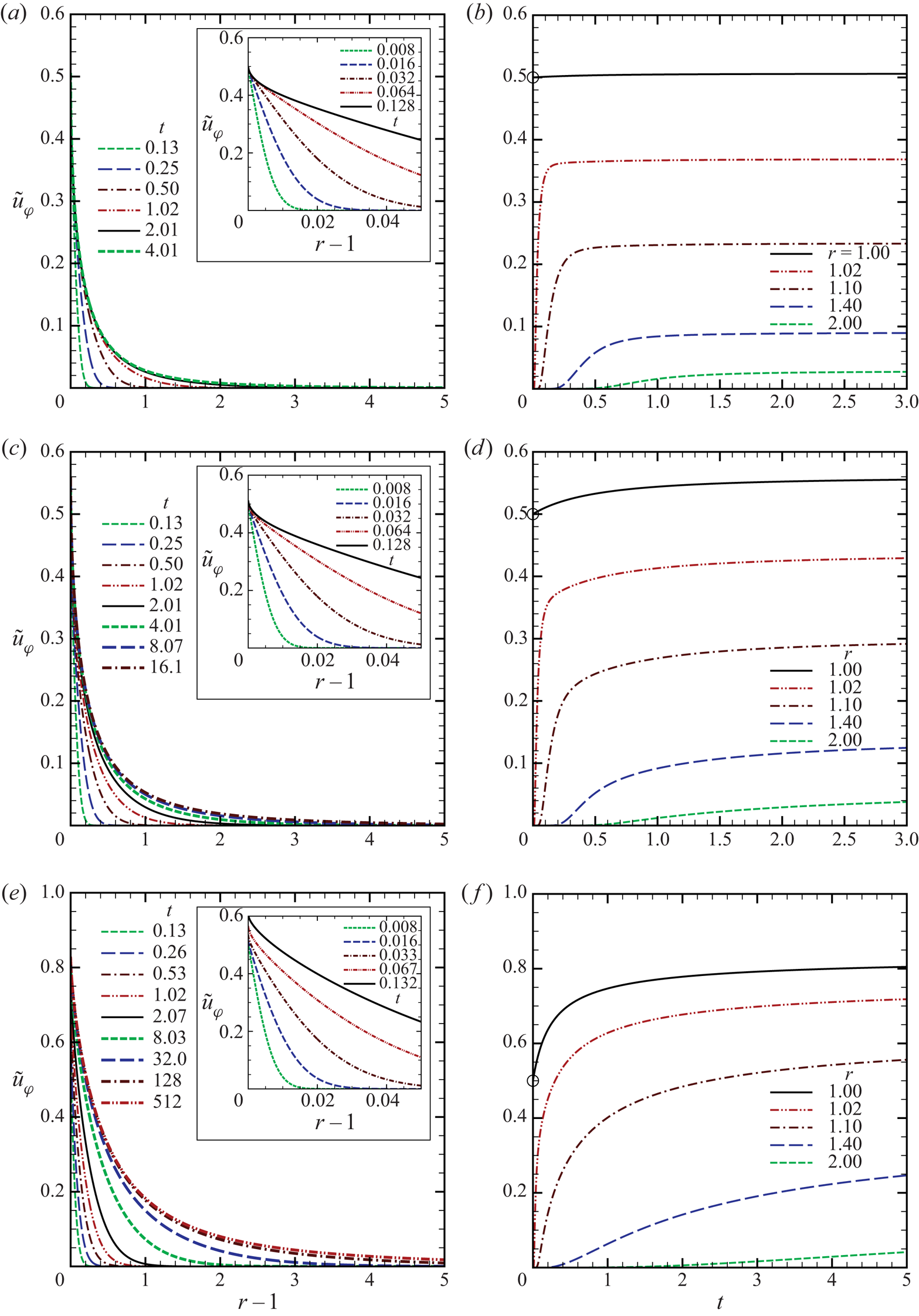
Figure 5. The profiles of the circumferential velocity for various  $k$: (a,b) $k=10$; (c,d) $k=1$; (e,f) $k=0.1$. Panels (a,c,e) show $\tilde {u}_{\varphi }$ versus $r$ for various $t$, while panels (b,d,f) show $\tilde {u}_{\varphi }$ versus $t$ for various $r$. The insets in panels (a,c,e) show a close-up near the sphere, and the symbol $\circ$ in panels (b,d,f) indicates the limiting value at $t \to 0_+$ along $r=1$.

Figure 6. The profiles of the tangential stress for various  $k$: (a,b) $k=10$; (c,d) $k=1$; (e,f) $k=0.1$. Panels (a,c,e) show $\tilde {P}_{r\varphi }$ versus $r$ for various $t$, and panels (b,d,f) show $\tilde {P}_{r\varphi }$ versus $t$ for various $r$. See the caption of figure 5.
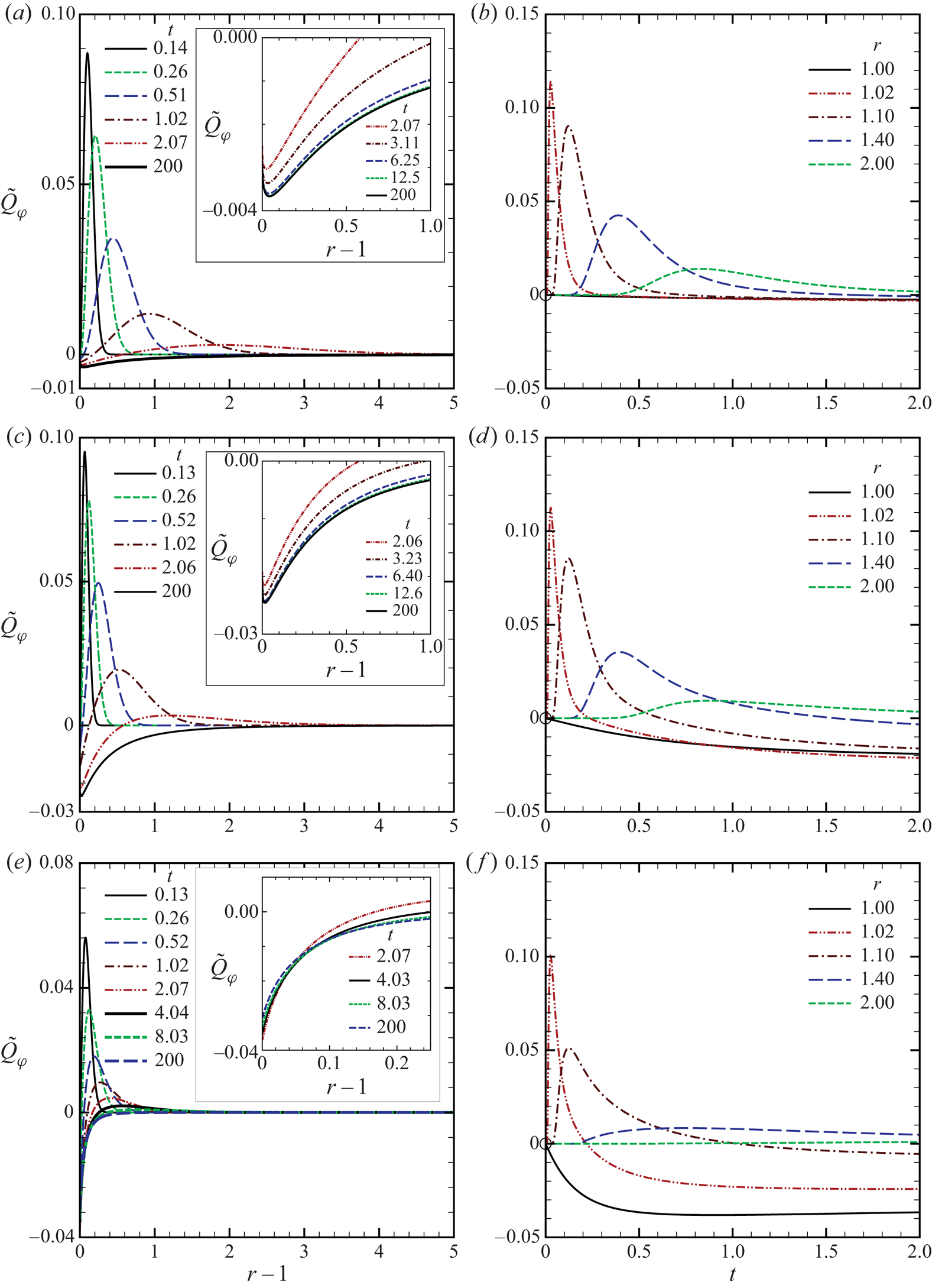
Figure 7. The profiles of the circumferential heat flow for various  $k$: (a,b) $k=10$; (c,d) $k=1$; (e,f) $k=0.1$. Panels (a,c,e) show $\tilde {Q}_{\varphi }$ versus $r$ for various $t$, and panels (b,d,f) show $\tilde {Q}_{\varphi }$ versus $t$ for various $r$. See the caption of figure 5.
The disturbance caused by the sphere rotation propagates into the gas as time goes on. The flow velocity on the sphere ( $r=1$) is exactly 0.5 for the free molecular gas, 1 for the continuum flow (the Stokes equation with no-slip boundary condition) and is between 0.5 and 1 for $0 < k < \infty$. The flow velocity gradually increases with time in the whole gas region. The disturbance propagates into the gas more slowly when $k$ is smaller (see panels b,d,f). However, the influence of the sphere rotation penetrates deeper into the gas when $k$ is smaller and the gas attains a larger rotational speed overall for smaller $k$.
$k$.
The value of the shear stress  $\tilde {P}_{r\varphi }$ is larger for large $k$. It increases abruptly after the onset of the self-rotation near the sphere and then decreases gradually with time. The disturbance propagates into the gas more slowly when $k$ is smaller, as in the case of $\tilde {u}_\varphi$ (see panels b,d,f).
The heat flux is localized in the vicinity of the sphere immediately after the onset of the self-rotation; it flows in the same direction as the sphere rotation and forms a peak-like profile near the boundary. The region of positive heat flow gradually propagates into the gas and spreads out. At the same time,  $\tilde {Q}_{\varphi }$ decreases near the boundary and changes its sign to negative values, implying that the heat flow changes its flow direction in the opposite sense as the sphere rotation. The negative heat flow is more prominent for $k=1$ than for $k=10$ and gradually develops in the whole region as time goes on. It should be noted that no negative heat flow occurs for the free molecular gas, as can be verified from (5.2c). When $k=0.1$, the negative heat flow is even greater, and is more confined near the boundary. It may be noted that the heat flux is negative in the whole gas region in the steady state for $0 < k < \infty$ (Taguchi et al. Reference Taguchi, Saito and Takata2019).
These features, particularly those in the initial stage near the boundary, are summarized in figure 8, where the isolines of (a)  $\tilde {u}_{\varphi }$, (b) $\tilde {P}_{r\varphi }$ and (c) $\tilde {Q}_{\varphi }$ are plotted in the $r$–
$r$– $t$ plane for $k=0.1$. We clearly see that the contour lines accumulate near the origin, indicating that the steep spatial and temporal variations take place in the vicinity of $(r,t)=(1,0)$. The reason of this abrupt change was discussed in the last paragraph of § 3.
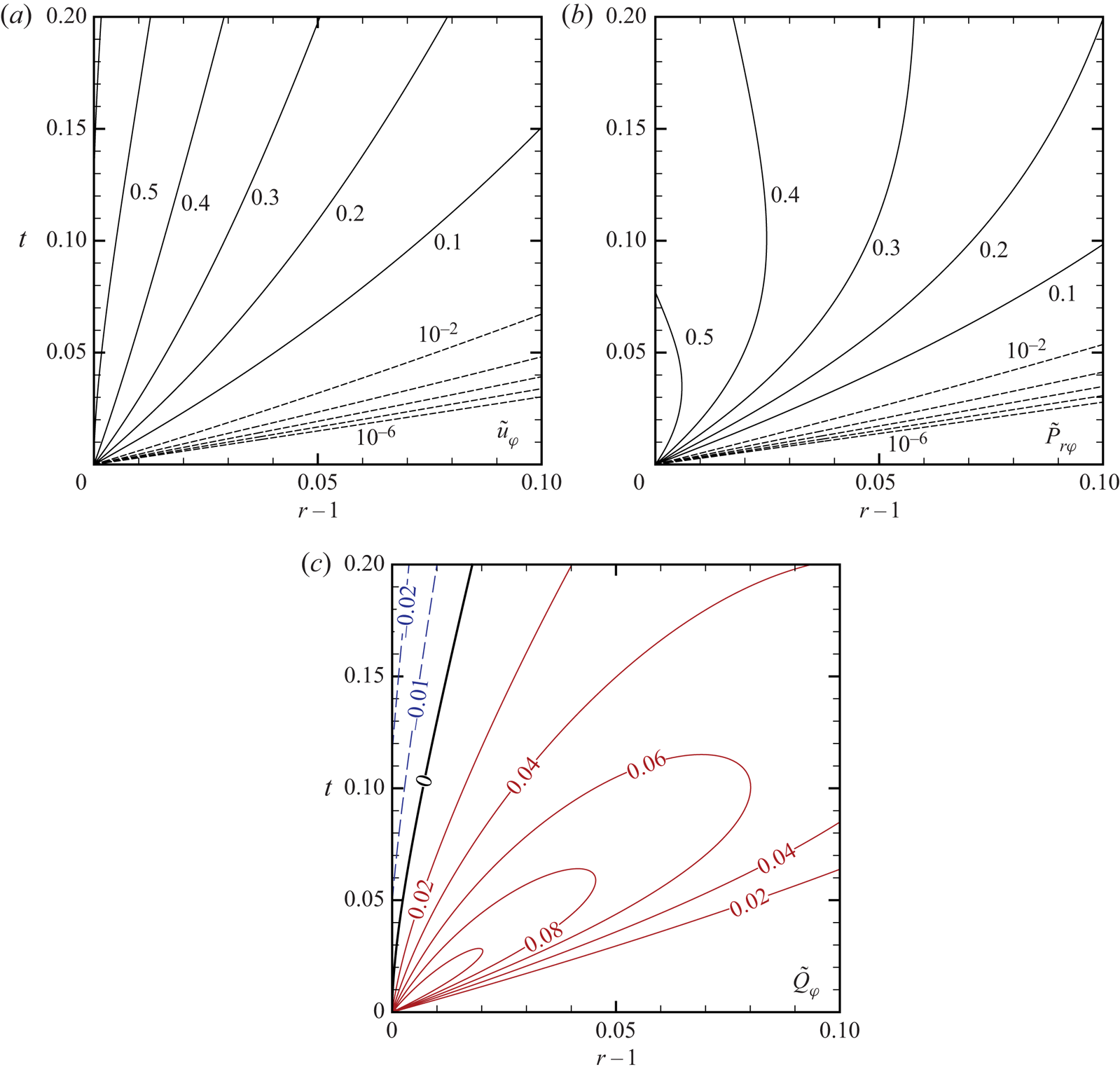
Figure 8. The overview of the macroscopic quantities for  $k=0.1$ near the sphere immediately after the onset of the rotation: (a) $\tilde {u}_{\varphi }$; (b) $\tilde {P}_{r\varphi }$; (c) $\tilde {Q}_{\varphi }$. The dashed line is used to indicate the values at $10^{-2}$, $10^{-3}$, …, $10^{-6}$ in panels (a,b). The solid (or dashed) line is used for positive (or negative) contour values in panel (c).
6.2. Long-time behaviour
In this section, we discuss the long-time behaviour of the macroscopic quantities. In figure 9 the behaviours of the macroscopic quantities are shown until relatively large time ( $t\approx 2500$) for $k=1$. More specifically, figure 9(a–c) show the circumferential component of the flow velocity $\tilde {u}_{\varphi }$, the shear stress $\tilde {P}_{r\varphi }$, and the circumferential component of the heat-flow vector $\tilde {Q}_{\varphi }$ as functions of $r$ for various times. The steady solution obtained by a hybrid method combining the finite-difference method and the method of characteristics (Taguchi et al. Reference Taguchi, Saito and Takata2019) is also included in each panel. We can observe that the profile of each macroscopic variable approaches the corresponding steady solution as time is increased.
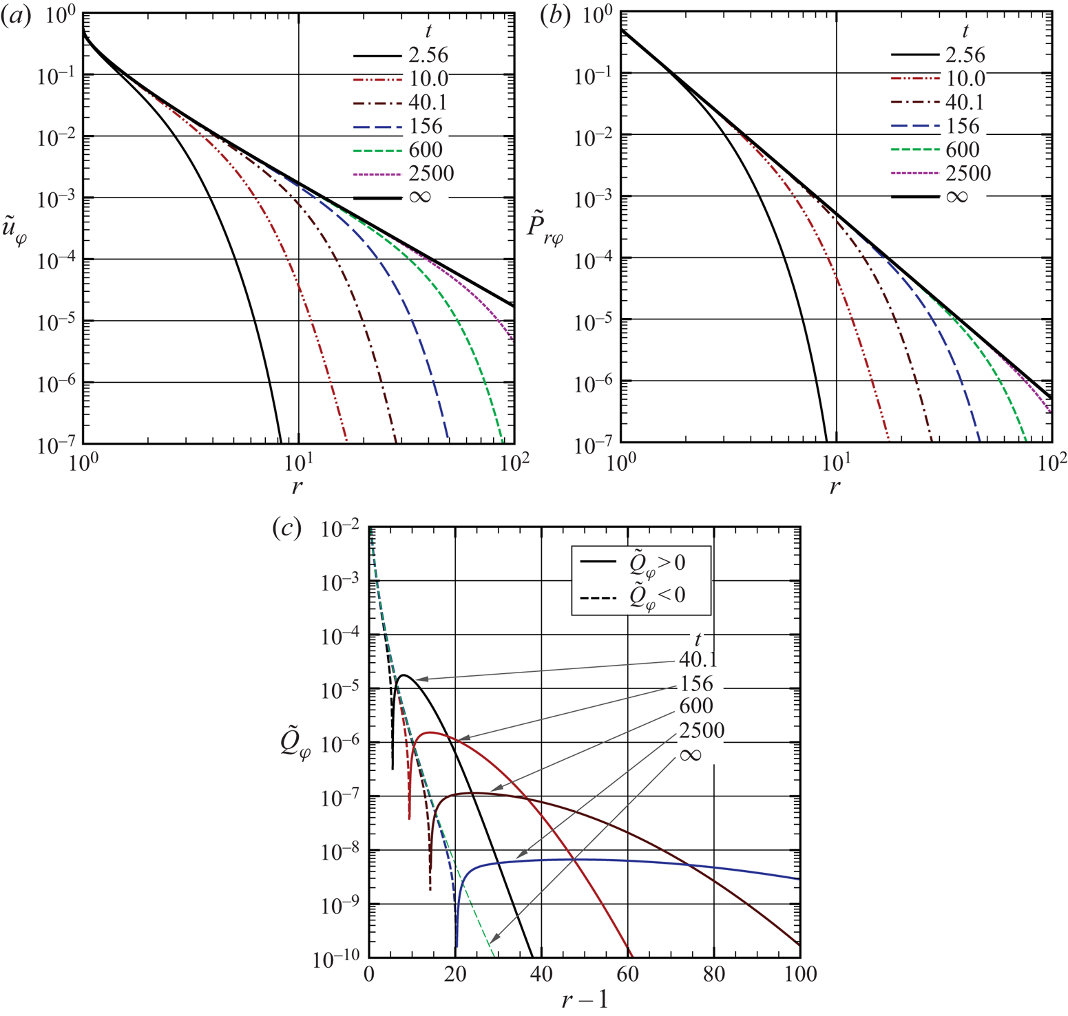
Figure 9. The profiles of the macroscopic quantities for various time  $t$ in the case of $k=1$: (a) $\tilde {u}_{\varphi }$; (b) $\tilde {P}_{r\varphi }$; (c) $\tilde {Q}_{\varphi }$. The steady solution ( $t=\infty$) is represented by the thick solid curve in panels (a,b) and by the thin broken curve in panel (c). In panel (c), the solid curve represents the part $\tilde {Q}_{\varphi } > 0$, while the broken curve the part $\tilde {Q}_{\varphi } < 0$.
In figure 9(c), where the semilogarithmic plot of  $|\tilde {Q}_{\varphi }|$ versus $r$ is shown, the positive and negative parts of $\tilde {Q}_{\varphi }$ are represented by the solid and broken curves, respectively. Note that, in the steady state, $\tilde {Q}_{\varphi }$ is everywhere negative. At $t=2500$, the curve almost overlaps with the steady solution in the part $r \lesssim 20$. The positive part of $\tilde {Q}_{\varphi }$ keeps travelling in the $r$ direction as time goes on, while decreasing its height and increasing the width (see also figure 7a,c,e).
To obtain further information on the long-time behaviour, we show in figure 10 the time derivative of each macroscopic variable as a function of  $t$ for various $r$: (a) $\partial \tilde {u}_{\varphi }/\partial t$; (b) $\partial \tilde {P}_{r\varphi }/\partial t$; and (c) $\partial \tilde {Q}_{\varphi }/\partial t$. From panels (a,b), it is clearly seen that $\partial \tilde {u}_{\varphi }/\partial t$ and $\partial \tilde {P}_{r\varphi }/\partial t$ tend to decay in proportion to $t^{-5/2}$ for large $t$. The time derivative of the heat flow $\partial \tilde {Q}_{\varphi }/\partial t$ is also likely to decay in proportion to $t^{-5/2}$ for $t \gg 1$, although it is more difficult to see the tendency. Thus, the rate of approach of the macroscopic quantities to the steady profiles is $t^{-3/2}$.

Figure 10. The time derivative of the macroscopic quantities  $\partial h/\partial t$ versus $t$ for various $r$ (
$r$ ( $k=1$): (a) $h = \tilde {u}_{\varphi }$; (b) $h = \tilde {P}_{r\varphi }$; (c) $h = \tilde {Q}_{\varphi }$.
Figure 11 contains further information on the approach of the macroscopic quantities to the steady state for different  $k$. Here, we show the slope of the double-logarithmic plot of $\partial h/\partial t$ versus $t$ at $r=1$ for various $k$, where $h=\tilde {u}_{\varphi }$ or $\tilde {Q}_{\varphi }$. We computed the slope $\alpha$ by applying a standard finite difference. If we do so, however, we observed a fluctuation developed after some moment, which is attributed to rounding errors. The fluctuated raw data are shown for $k=0.1$ in each panel by grey lines. Note that the slope for $\tilde {Q}_{\varphi }$ is more fluctuated than that of $\tilde {u}_{\varphi }$ because the magnitude of $\partial \tilde {Q}_{\varphi }/\partial t$ is much smaller. To smooth out the data, we took a moving average over 100 dimensionless times. The data thus obtained are shown by the symbols in the figures. The figure for $h=\tilde {P}_{r\varphi }$, which is similar to that of $\tilde {u}_{\varphi }$, is omitted here. It is seen from the figure that the slope tends to approach $\alpha =-5/2$ as the time proceeds, irrespective of $k$. This confirms the exponent of $t^{-3/2}$ in the long-time behaviour.

Figure 11. The temporal variation of the slope  $\alpha$ of $\ln |\partial h/\partial t| \sim \alpha t + \textrm {const.}$, where $h = \tilde {u}_{\varphi }$ or $\tilde {Q}_{\varphi }$ at $r=1$ for various $k$: (a) $h=\tilde {u}_{\varphi }$; (b) $h= \tilde {Q}_{\varphi }$. The moving averages over 100 dimensionless times are shown by the symbols, which are connected by the solid lines. The fluctuated raw data are shown for $k=0.1$ by grey lines.
6.3. Torque acting on the sphere
In this section, we discuss the transient behaviour of the torque acting on the rotating sphere. Figure 12(a) shows the time evolution of  $-h_M$ for various $k$ (
$k$ ( $-h_M$ is shown instead of $h_M$). The (dimensionless) torque $-h_M$ is constant in time for the free molecular gas, and is monotonically decreasing in $t$ for $k < \infty$. It attains its supremum at $t=0_+$, which coincides with the value for the free molecular gas. In case of $k<\infty$, after the onset of the rotation, $-h_M$ undergoes a rapid decrease in proportion to $t$ followed by a subsequent slower decay in proportion to $t^{-3/2}$ approaching the final steady state.

Figure 12. The (dimensionless) torque acting on the sphere. (a) The  $-h_M$ versus $t$ is shown for various $k$. Here, $k=\infty$ indicates the result for the free molecular gas. (b) A comparison between the numerical (solid) and the asymptotic (dash-dotted and dashed) solutions for $k=0.1$ and $0.01$ over a wide range of $t$. Equation (5.19) is shown by the dash-dotted curve and (5.19) with $b_1^{(1)}=0$, which corresponds to the continuum flow (i.e. the Stokes equation with no-slip boundary condition), is shown by the dashed curve. The asymptotic formula for the steady solution ((4.4b) in Taguchi et al. (Reference Taguchi, Saito and Takata2019)), which includes second-order slip corrections, is shown by the horizontal long-dashed line. Note that the asymptotic formula (5.19) is valid only for $t\gtrsim k^{-1}$.
In figure 12(b), we compare the numerical solution and the asymptotic formula (5.19) for small  $k$ for a wider range of $t$ (
$t$ ( $k=0.1$ and $0.01$). Here, the solid curves represent our numerical results, while the dash-dotted curves the asymptotic formula (5.19). A favourable agreement is observed for $k=0.01$ except for small values of $t ({\lesssim }1)$. In the case of $k=0.1$, the discrepancy is noticeable but the shape of the curve is well represented by the asymptotic expression. For comparison, we also show the result based on (5.19) with $b_1^{(1)}=0$ by the dashed curve, which corresponds to the continuum flow (i.e. the Stokes equation with no-slip boundary condition). The deviation is more prominent, particularly for $k=0.1$. Note that the asymptotic formula is valid for $t \gtrsim k^{-1}$. Nevertheless, a reasonable agreement between the numerical and asymptotic results is observed even for smaller values of $t$.
$t$.
The approach to the steady torque is algebraic and is proportional to  $t^{-3/2}$ for $t \gg 1$. Thus, the tangential stress on the sphere $\tilde {P}_{r\varphi }$ for $t\gg 1$ can be approximated by a function
 \begin{equation} \tilde{P}_{r\varphi} = \mathcal{P}_0 + \mathcal{P}_1 t^{-3/2} + o(t^{-3/2}), \quad r=1, \end{equation}
where  $\mathcal {P}_0$ and $\mathcal {P}_1$ are constants which depend on $k$. The $\mathcal {P}_0$ and $\mathcal {P}_1$ can be obtained by fitting the first two terms of the above expression with the numerical data of $\tilde {P}_{r\varphi }(1,t)$ for large $t$. It turned out that adding a third term, $\mathcal {P}_2 t^{-5/2}$, gives a better fitting result. Then, the coefficients $(\mathcal {P}_0,\mathcal {P}_1,\mathcal {P}_2)$ were obtained by the least squares method, where the numerical data for $t \gtrsim 10^{2}$ were used for $k \geqslant 0.1$ and those for $t\gtrsim 8\times 10^{2}$ for $k<0.1$. Note that the presence of the $t^{-5/2}$-term can be verified in the case of the continuum flow from (5.17). The results thus obtained are summarized in figure 13 and in table 3 for $\mathcal {P}_0$ and $\mathcal {P}_1$. It should be noted that $\mathcal {P}_0$ corresponds to $\lim _{t\to \infty }\tilde {P}_{r\varphi }|_{r=1}$ which can also be obtained from the steady solution (Taguchi et al. Reference Taguchi, Saito and Takata2019). The latter, obtained by a numerical method different from the present approach, is also included in table 3 for comparison. As seen from the table, $\mathcal {P}_0$ obtained by the fitting agrees well with the stationary result. The solid curve in figure 13(a) is the asymptotic formula for $k \ll 1$ for the steady solution ((4.4b) in Taguchi et al. (Reference Taguchi, Saito and Takata2019)). The $\mathcal {P}_1$ is decreasing in $k$ and, thus, decays faster for larger $k$. The coefficient $\mathcal {P}_1$ is likely to behave as $\mathcal {P}_1 \propto k^{-5/2}$ for $k \gg 1$ (see figure 13b). On the other hand, $\mathcal {P}_1$ for small $k$ is approximated by
 \begin{equation} \mathcal{P}_1 = \left(\frac{2}{{\rm \pi} \gamma_1 k}\right)^{1/2}, \quad k \ll 1, \end{equation}
(see (5.21d)), where  $\gamma _1=1$ for the BGK model. Equation (6.2) is shown in figure 13(b) by the dashed line.
Figure 13. The coefficients  $\mathcal {P}_0$ and $\mathcal {P}_1$ in (6.1): (a) $\mathcal {P}_0$ versus $k$; (b) $\mathcal {P}_1$ versus $k$. The symbol $\circ$ shows the numerical result. In panel (a), the dashed line indicates the value at $k\to \infty$ (the free molecular flow), while the solid curve the asymptotic formula for $k\ll 1$ for the steady solution ((4.4b) in Taguchi et al. (Reference Taguchi, Saito and Takata2019)). In panel (b), the solid line indicates (6.2), while the broken line the slope corresponding to $\mathcal {P}_1 \propto k^{-5/2}$.
Table 3. The values of  $\mathcal {P}_0$ and $\mathcal {P}_1$ in (6.1) (see also figure 13). The values in parentheses are those obtained from the steady solution (Taguchi et al. Reference Taguchi, Saito and Takata2019).
 $^{a}$The results obtained by the asymptotic formula (4.4b) in Taguchi et al. (Reference Taguchi, Saito and Takata2019).
7. Discussion
We have seen that the circumferential heat flow is induced by the rotation of the sphere. Let us first discuss its initial peak-like behaviour localized near the boundary. We know that the heat flow is given by (5.2c) in the case of a free molecular gas. If we consider the limit  $t \to 0$ such that $(r-1)/t = \textrm {const.}$, this reduces to
 \begin{equation} \tilde{Q}_{\varphi} = \frac{1}{2\sqrt{\rm \pi}} \frac{r-1}{t} \exp\left(-\frac{(r-1)^{2}}{t^{2}}\right). \end{equation}
Note that the above expression describes the heat flow induced by an impulsive onset of a uniform tangential motion of a flat plate in a collisionless gas (i.e. one-dimensional linearized Rayleigh problem for a free molecular gas), if  $r-1$ is interpreted as the distance from the plate. On the other hand, in the case of a finite $k < \infty$, it can be shown that the heat flow is also described by (7.1) as the same limit $t \to 0_+$ is approached. To see this, let us consider the following change of variables:
 \begin{gather} y = \frac{r-1}{\varepsilon}, \quad \zeta_y = \zeta_r, \quad \zeta_x = \zeta_\varphi, \quad \zeta_z = \zeta_\theta, \quad \hat{\tau} = \frac{t}{\varepsilon}, \end{gather}
 \begin{gather}\phi_1(y,\zeta_y,\zeta,\hat{\tau}) = \phi_S(1+\varepsilon y,\zeta_y,\zeta,\varepsilon \hat{\tau}), \end{gather}
where  $\varepsilon$ is a small positive number that has been introduced to make $y$ and $\hat {\tau }$ of the order of unity. The $\phi _1$ satisfies the equation
 \begin{gather} \frac{\partial \phi_1}{\partial \hat{\tau}} + \zeta_y \frac{\partial \phi_1}{\partial y} + \frac{\varepsilon (\zeta^{2} - \zeta_y^{2})}{1+ \varepsilon y} \frac{\partial \phi_1}{\partial \zeta_y} - \frac{\varepsilon \zeta_y}{1+\varepsilon y} \phi_1 = \frac{\varepsilon}{k} L_1(\phi_1), \end{gather}
 \begin{gather}L_1(\phi_1) = -\phi_1 + 2 u_x, \end{gather}
 \begin{gather}u_x = \tfrac{1}{2} \langle (\zeta^{2} - \zeta_y^{2}) \phi_1 \rangle, \end{gather}
where  $\zeta = (\zeta _x^{2} + \zeta _y^{2} + \zeta _z^{2})^{1/2}$. Applying the same coordinate transformation to the boundary condition at $r=1$ as well as to the initial condition, we see that the problem is reduced to a one-dimensional Rayleigh problem for a collisionless gas so far as the leading-order terms in $\varepsilon$ are concerned. In this way, the initial behaviour of the heat flow in the vicinity of the sphere is reduced to (7.1), irrespective of the values of $k < \infty$.
We note that  $\tilde {Q}_\varphi$ of (7.1) is self-similar in $(r-1)/t$ (or $y/\hat {\tau }$), non-negative and approaches zero as $r \to 1$ or $r \to \infty$ when $t>0$ is fixed. Consequently, the maximum value does not change in time, which is $1/2 \sqrt {2\textrm {e}{\rm \pi} }$, while the profile becomes wider as $t$ is increased. In this manner, the initially localized peak near the sphere spreads into the gas. As $t$ (and $r$) is increased, $\varepsilon$ becomes no longer small, and the curvature effect as well as molecular collision begins to play a role. As a result, $\tilde {Q}_{\varphi }$ starts to behave differently from that of the one-dimensional free molecular solution. This behaviour near the origin $(r,t)=(1_+,0_+)$ is also consistent with the discussion given at the end of § 3.
Next, we discuss the behaviour of the heat flow  $Q_\varphi$ at relatively large $t$ by restricting ourselves to the case of small $k$. Figure 14(a) shows a comparison of the numerical result with the asymptotic formula (5.18) for $k=0.05$ and $0.01$ in the region close to $r=1$ at $t=100$. The agreement between the numerical solution and the asymptotic solution is good, motivating us to discuss the behaviour of $Q_\varphi$ for small $k$ based on the asymptotic theory. In the present problem, the most significant term in the asymptotic expansion $Q_\varphi = Q_{\varphi H0} + k (Q_{\varphi H1} + Q_{\varphi K1}) + k^{2} (Q_{\varphi H2} + Q_{\varphi K2}) + \cdots$ is $k Q_{\varphi K1}$, since $Q_{\varphi H0}$ and $Q_{\varphi H1}$ are identically zero (see the caption of table 2). The heat conduction due to Fourier's law is irrelevant since the temperature is uniform. The contribution of $k Q_{\varphi K1}$, describing the Knudsen layer adjacent to the boundary, is shown by the dashed curves in the figure. This heat flow in the Knudsen layer does not vanish as $t \to \infty$ and contributes to the negative heat flows in the long-time limit, as mentioned in § 5.2. Note also that the magnitude of the heat flow is proportional to $k$. Therefore, it is of the same order as the shear stress, although there is an essential difference in that the heat flow is confined in the Knudsen layer while the shear stress extends over the gas region.

Figure 14. The behaviour of the heat flow  $Q_\varphi$ for small $k$. (a) Profiles of $\tilde {Q}_\varphi ({=}Q_\varphi /\varOmega \sin \theta )$ for $k=0.01$ and $0.05$ at $t=100$ in the vicinity of $r=1$. (b) Profiles of $\tilde {Q}_\varphi ({=} Q_\varphi /\varOmega \sin \theta )$ for $k=0.01$ at various $t$ ranging from $t=100$ to 1000. Note the difference between the scales of panels (a,b) in the ordinate. In panels (a,b), the solid curve represents the numerical solution of the BGK equations, the dash-dotted curve the asymptotic formula (5.18) and the dashed curve the leading-order term $k Q_{\varphi K1}$ in the asymptotic solution (see table 2). The inset in panel (a) is a close-up of the case $k=0.01$ near $r=1$. In panel (b) the profiles of $k Q_{\varphi K1} + k^{2} Q_{\varphi H2}$ (with no second-order Knudsen-layer correction included) are also shown by the (green) long-dashed curves, which overlap with the dash-dotted curves representing (5.18).
The second-order Hilbert part  $k^{2} Q_{\varphi H2}$ in the heat flow merits some attention. The origin of this term is the Laplacian of the flow velocity (see (16b) in Takata & Hattori (Reference Takata and Hattori2012)), which reduces to $Q_{\varphi H2} = \frac {1}{2} (\gamma _3/\gamma _1) \partial u_{\varphi H0}/ \partial s$, $s = kt$, by the use of (5.12) in the present case. Hence, this second-order gas-rarefaction effect is related to the transient behaviour (and therefore vanishes in the steady state, i.e. $t \to \infty$). The term is included in the asymptotic solution shown in figure 14(a) (dash-dotted curve). However, its modulus is much smaller than the typical magnitude of $k Q_{\varphi K1}$ at $t=100$, and it cannot be distinguished in the figure. To see the contribution of the Hilbert part more clearly, the narrow region around $\tilde {Q}_\varphi = 0$ in figure 14(a) is stretched in figure 14(b) for $k=0.01$, where the solutions for other $t$ are also plotted until $t=1000$. Note the difference between the scales of figures 14(a) and 14(b) in the ordinate. Although very small, the spreading and decreasing tendency of the circumferential heat flow outside the Knudsen layer is well described by the time derivative of the overall circumferential flow velocity $u_{\varphi H0}$.
We close this section by presenting the leading-order heat flow  $k Q_{\varphi K1}$, (5.18) with $\gamma _3 = \mathcal {H}^{(1)} = b_1^{(1)}=0$ (see table 2), in a dimensional form for a steady state ( $t \to \infty$). Let us denote the (dimensional) heat-flow vector by $\boldsymbol {q}$. Noting the relation between $k$ and the viscosity $\mu _0$ (see the sentence after (5.12)), $\boldsymbol {q}$ in the steady state is expressed as
 \begin{equation} \boldsymbol{q} = -3 \mu_0 (2RT_0)^{1/2} \left(\boldsymbol{\varOmega}^{*} \times \frac{\boldsymbol{x}^{*}}{|\boldsymbol{x}^{*}|}\right) \frac{1}{\gamma_1} H_1^{(1)}\left(\frac{\gamma_1 p_0}{\mu_0 (2RT_0)^{1/2}}(|\boldsymbol{x}^{*}|-L)\right), \end{equation}
where  $\boldsymbol {\varOmega }^{*}$ and $\boldsymbol {x}^{*}$ are the angular velocity of the sphere and the position vector, respectively. From this formula, we clearly see that the magnitude of the (steady) heat flow is proportional to the viscosity.
8. Concluding remarks
In this paper, we investigated the transient behaviour of a rarefied gas caused by an impulsive onset of the rotating motion of a sphere based on the linearized BGK equation and the diffuse reflection boundary condition. This problem can be viewed as an extension of the one-dimensional linearized Rayleigh problem to a three-dimensional axisymmetric flow. Special attention was paid to the propagation of the discontinuity of VDF in the phase space. For this purpose, we carried out a numerical analysis based on the integral form of the BGK equation. Our findings are summarized as follows.
(i) The behaviours of the macroscopic quantities have been clarified for a wide range of the Knudsen number including the free molecular flow and the continuum flow.
(ii) The heat flow, which is initially localized near the boundary and flows in the same direction as the sphere rotation, spreads into the gas as time goes on. As the final steady state is approached, the region with negative heat flow, flowing in the opposite direction as the sphere rotation, is established.
(iii) (The long-time behaviour.) The rate of approach of the macroscopic quantities to the steady state is in proportion to
$t^{-3/2}$ for $t \gg 1$. In other words, the gas-rarefaction effect does not change the decaying rate and the degree of gas rarefaction (the Knudsen number) affects merely the proportionality constant. The free molecular flow is an exception.(iv) The transient behaviour of the torque on the sphere is clarified. For large
$t \gg 1$, the magnitude of the term proportional to $t^{-3/2}$ becomes small in proportion to $k^{-5/2}$ for $k \gg 1$, indicating the faster approach to the steady torque for larger $k$.


Acknowledgements
This work was supported by JSPS KAKENHI grant no. 17K06146 and no. 20H02067.
Declaration of interests
The authors report no conflict of interest.
Appendix A. Lattice systems and accuracy of numerical computations
In this appendix, we give explicit formulae for the lattice system used in the present computations, and comment on the accuracy.
The grid points for  $r$ and $t$ variables are defined by the formulae (see (4.5))
 \begin{equation} g_\gamma(x) = \begin{cases} \delta_{\gamma r} + a_\gamma( \exp(b_\gamma x^{2}) - 1 ), & 0 \leqslant x \leqslant \check{N}_\gamma,\\ \delta_{\gamma r} + c_\gamma x + d_\gamma, & \check{N}_\gamma < x \leqslant N_\gamma, \end{cases} \end{equation}
where  $\gamma = r$ or $t$,
$t$,
 \begin{gather} \delta_{\gamma r} =\begin{cases} 1, & \gamma=r, \\ 0, & \gamma=t, \end{cases} \end{gather}
 \begin{gather}b_\gamma = \ln( \varDelta_{min,\gamma}/a_\gamma + 1 ),\quad \text{with}\ (\varDelta_{min,r}, \varDelta_{min,t}) = (10^{-8},10^{-10}), \end{gather}
 \begin{gather}\check{N}_\gamma = \lfloor b_\gamma^{-1} \ln( \check{\gamma}/a_\gamma + 1) \rfloor\quad \text{with}\ (\check{r},\check{t}) = (40,1), \end{gather}
 \begin{gather}c_\gamma = 2 a_\gamma b_\gamma \check{N}_\gamma \exp( b_\gamma \check{N}_\gamma^{2}), \quad d_\gamma = a_\gamma ( \exp( b_\gamma \check{N}_\gamma^{2} ) - 1 ) - c_\gamma \check{N}_\gamma, \end{gather}
and  $N_\gamma$ and $a_\gamma$ are positive constants which are suitably chosen depending on $k$. Note that $g_\gamma (1) - g_\gamma (0) = \varDelta _{min,\gamma }$ and that the two functions appearing in $g_\gamma (x)$ are smoothly connected at $x = \check {\gamma }$, where $g_\gamma (\check {N}_\gamma ) \approx \check {\gamma }$. Typical choices of $a_\gamma$ and $N_\gamma$ are summarized in table 4 along with the values of $(r_{max},t_{max}) = (g_r(N_r), g_t(N_t))$ and $(c_r,c_t)$.
Table 4. Typical lattice systems for the space variable  $r$ as well as for the time variable $t$.
$t$.
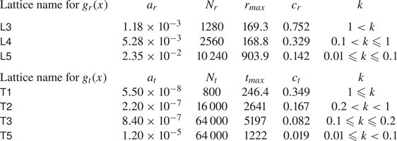
The grid points for  $\theta _\zeta$, $\zeta$ and $\tilde {t}$ are regenerated at every time step in an adaptive manner. We omit details on the grids for these variables.
We have checked the accuracy of our numerical computations in various ways, for instance, by changing the number of grid points, grid parameters, etc. Here, we provide some numerical data to assess the present computations based on the conservation law. As shown in (2.11), the quantity on the left-hand side should be identically zero, while it is not in an actual numerical computation due to numerical errors. Thus, the deviation from zero is a measure of computational accuracy. Let us introduce
 \begin{equation} \mathcal{I}(r,t) = \dfrac{\left|\dfrac{\partial {u}}{\partial {t}}+\dfrac{1}{2r^{3}}\dfrac{\partial {}}{\partial {r}}(r^{3} \tilde{P}_{r\varphi})\right|}{\sqrt{\left(\dfrac{\partial {u}}{\partial {t}}\right)^{2} +\left(\dfrac{1}{2r^{3}}\dfrac{\partial {}}{\partial {r}}(r^{3} \tilde{P}_{r\varphi})\right)^{2}}}, \end{equation}
and
 \begin{equation} \bar{\mathcal{I}} = \frac{1}{t_{max}}\int_0^{t_{max}} \left(\frac{1}{\dfrac{4}{3}{\rm \pi} r_{max}^{3}} \int_{1}^{r_{max}}\mathcal{I}(r_1,t_1) (4{\rm \pi} r_1^{2}) \,\mathrm{d} r_1 \right) \mathrm{d} t_1. \end{equation}
Then, for some typical values of  $k$, we have
 \begin{equation} \bar{\mathcal{I}} \simeq \begin{cases} 1.3 \times 10^{-5} & (k=0.1), \\ 7.6 \times 10^{-6} & (k=0.2), \\ 4.6 \times 10^{-6} & (k=0.6), \\ 5.2 \times 10^{-3} & (k=1), \\ 6.1 \times 10^{-3} & (k=10), \end{cases} \end{equation}
for our numerical results.
We mention that a comparison of the values of  $\mathcal {P}_0$ listed in table 3 with those of Taguchi et al. (Reference Taguchi, Saito and Takata2019) (time-independent problem) gives also a measure of accuracy.


 Open access