


1. Introduction
1.1. Background
Thin-film equations are utilised in fluid dynamics when there exists a direction in which the aspect ratio can be considered small (Oron, Davis & Bankoff Reference Oron, Davis and Bankoff1997; Craster & Matar Reference Craster and Matar2009; Eggers & Fontelos Reference Eggers and Fontelos2015). Examples include bubble caps, tear films, ice sheets and lubrication configurations. In particular, thin-film equations have been used to consider flows influenced by surface tension variations (De Wit, Gallez & Christov Reference De Wit, Gallez and Christov1994; Breward Reference Breward1999; Timmermans & Lister Reference Timmermans and Lister2002; Bowen & Tilley Reference Bowen and Tilley2013; Kitavtsev, Fontelos & Eggers Reference Kitavtsev, Fontelos and Eggers2018). Such Marangoni flows are responsible for many different physical processes across varied lengthscales, such as the calming of surface ocean waves, tears of wine, and the decrease in velocity of a rising bubble (Manikantan & Squires Reference Manikantan and Squires2020).
Recently, Marangoni effects have been suggested as a potential mechanism for rupture of surface bubbles (Poulain, Villermaux & Bourouiba Reference Poulain, Villermaux and Bourouiba2018), which refers to bubbles that rest near a liquid–vapour interface. The caps of such surface bubbles are thin liquid films. It has been noted theoretically (Bowen & Tilley Reference Bowen and Tilley2013; Kitavtsev et al. Reference Kitavtsev, Fontelos and Eggers2018) and experimentally (Néel & Villermaux Reference Néel and Villermaux2018) that a sufficiently large local deposition of surfactants or (heat) onto a liquid film is enough to rupture the film. Surface bubble rupture is of importance in industry, health (Bourouiba Reference Bourouiba2021), volcanic activity (Gonnermann & Manga Reference Gonnermann and Manga2007; Nguyen et al. Reference Nguyen, Gonnermann, Chen, Huber, Maiorano, Gouldstone and Dufek2013) and ocean–atmosphere interaction (Veron Reference Veron2015; Deike Reference Deike2022). Once emitted in the atmosphere, aerosols formed from the rupture of ocean surface bubbles can serve as cloud condensate nuclei and affect the radiative balance of Earth.
In studies of thin films influenced by Marangoni effects, top–bottom symmetry is often assumed (De Wit et al. Reference De Wit, Gallez and Christov1994; Bowen & Tilley Reference Bowen and Tilley2013; Kitavtsev et al. Reference Kitavtsev, Fontelos and Eggers2018). In practice, asymmetric, i.e. top to bottom in the case of a horizontal sheet and side to side in the case of a vertical sheet, distributions of surfactants, or surface tension more generally, are possible. An immediate consequence of assuming symmetry is that the bending of the sheet, i.e. the centreline deformation, is ignored. For a nonlinear surface tension isotherm  $\sigma = \sigma (\varGamma )$, indicating how surface tension $\sigma$ varies with surfactant concentration $\varGamma$, we expect that $\sigma (\varGamma ) \neq 2\sigma (\tfrac {1}{2}\varGamma )$ in general. Thus, modelling an asymmetric set-up, e.g. surfactant concentration $\varGamma$ on the top surface and zero surfactant concentration on the bottom surface, with a symmetric configuration, where the surfactant concentration is $\tfrac {1}{2}\varGamma$ on both the top and bottom surfaces, may potentially lead to inaccurate tangential Marangoni forces, which will be discussed in § 4.6 below.
We consider the extensional flow regime, where the velocity (and pressure) in the direction of the large length scale can be taken to be roughly independent of the small direction. This flow regime is amenable to theoretical analysis but places restrictions (see § 3.2) on the magnitude of the Reynolds number (comparing inertia and viscous forces), Marangoni number (comparing Marangoni and viscous forces) and capillary number (comparing viscous and capillary forces).
The broken symmetry in surface tension means that the bending of the sheet should be considered. Centreline deformation of thin films has been discussed in the literature. For example, a heavy liquid filament sags under the influence of gravity (Teichman & Mahadevan Reference Teichman and Mahadevan2003). Folding liquid sheets are also an example (Ribe Reference Ribe2002, Reference Ribe2003). A well known phenomenon for thin liquid sheets with top–bottom asymmetry is the flapping of a retracting liquid sheet (Lhuissier & Villermaux Reference Lhuissier and Villermaux2009), which has been proposed recently to be relevant for the production of film drops (Jiang et al. Reference Jiang, Rotily, Villermaux and Wang2022).
In the context of surface bubbles, the inside of a bubble and the outside of a bubble can have different distributions of surfactants. Indeed, top–bottom asymmetry of a surface bubble with surfactants can be seen in numerical work by Atasi et al. (Reference Atasi, Legendre, Haut, Zenit and Scheid2020) and in experimental work by Zawala et al. (Reference Zawala, Miguet, Rastogi, Atasi, Borkowski, Scheid and Fuller2023). Theoretically, Shi, Fuller & Shaqfeh (Reference Shi, Fuller and Shaqfeh2022) considered the drainage of a surface bubble with surfactants, where their derivation also considered extensional flow with top–bottom asymmetry (without inertia, similar to Breward Reference Breward1999). In their subsequent analysis and experimental verification of their extensional flow equations, Shi et al. (Reference Shi, Fuller and Shaqfeh2022) assumed top–bottom symmetry in order to focus on important characteristics of non-axisymmetric drainage.
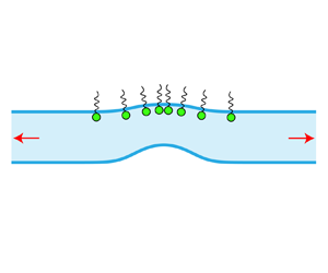
It should be noted that although surface bubbles serve as motivation for this study, flow in the film of a surface bubble cap may not be in the extensional flow regime. When shear stress increases in an otherwise free thin liquid film, e.g. by imposing a stronger surface tension gradient, the flow transitions (Champougny et al. Reference Champougny, Scheid, Restagno, Vermant and Rio2015; Atasi et al. Reference Atasi, Legendre, Haut, Zenit and Scheid2020) from the extensional flow regime, where the flow profile is plug-like, to the shear flow regime, where the flow profile is nearly parabolic (see figure 1). In particular, for surface bubbles, there are cases where the extensional flow regime is considered (Debrégeas, De Gennes & Brochard-Wyart Reference Debrégeas, De Gennes and Brochard-Wyart1998; Howell Reference Howell1999; Shi et al. Reference Shi, Fuller and Shaqfeh2022; Bartlett et al. Reference Bartlett, Oratis, Santin and Bird2023), cases in which the shear flow regime is considered (Lhuissier & Villermaux Reference Lhuissier and Villermaux2012), and cases where both the extensional flow and shear flow regimes are considered (Champougny et al. Reference Champougny, Roché, Drenckhan and Rio2016; Atasi et al. Reference Atasi, Legendre, Haut, Zenit and Scheid2020; Miguet et al. Reference Miguet, Pasquet, Rouyer, Fang and Rio2020). For example, extensional flow is usually only considered for surface bubbles with drainage at low Reynolds number (Debrégeas et al. Reference Debrégeas, De Gennes and Brochard-Wyart1998; Nguyen et al. Reference Nguyen, Gonnermann, Chen, Huber, Maiorano, Gouldstone and Dufek2013); such a regime is of interest in industry and volcanology. Thus, the examples provided in §§ 4 and 5 should be seen as a fundamental study in liquid film dynamics rather than directly representing the film flow of any given surface bubble cap.

Figure 1. Schematic diagram of the (a) extensional flow regime and (b) shear flow regime (non-extensional flow).
1.2. Outline of the paper
The paper is structured as follows. In § 2, the governing Navier–Stokes equations with corresponding boundary conditions are given. Then, in § 3, we give the asymmetric thin-film equations, including Marangoni effects, using an asymptotic expansion strategy from previous works (Howell Reference Howell1996; Breward Reference Breward1999), where the resulting equations extend equations already given by these authors. In §§ 4 and 5, we consider the example of the deposition of insoluble surfactants on one side of a liquid film. Specifically, in § 4, the liquid film is otherwise at rest and in § 5, the liquid film is otherwise uniformly thinning with a constant extension rate. We consider the case of low-Reynolds-number motions,  $ Re \ll 1$; see Appendix C for a brief discussion on including inertia.
1.3. Main results of the paper
The main results of the paper are as follows. First, analytical extensions to prior work is given for the relevant thin-film equations. For the surfactant deposition problem, analytical progress is made via transforming to Lagrangian coordinates, which allows us to (a) describe the evolution of the sheet, (b) discuss the effects of the shape of surfactant isotherms and (c) to discuss the possibility that satellite drops may be formed from pinching via Marangoni effects, such as when the initial surfactant isotherm has a double maximum.
2. Governing equations and boundary conditions
We consider an incompressible, two-dimensional Newtonian film (viscosity  $\mu$, density $\rho$) with the horizontal direction given by the $x$ axis and the vertical direction given by the $z$ axis. The top surface of the film is given by $z=H(x,t)+\tfrac {1}{2}h(x,t)$ and the bottom surface of the film is given by $z=H(x,t)-\tfrac {1}{2}h(x,t)$ (see figure 2). We assume that the fluid of the thin film is not coupled to the surrounding fluid; typically, the thin film is surrounded by air otherwise at rest.

Figure 2. Schematic of a thin film with curved centreline  $H(x,t)$ and thickness $h(x,t)$ (the $x$ axis is in the horizontal direction, the $z$ axis is in the vertical direction and $t$ is time). The top surface of the film is given by $z=H(x,t)+\tfrac {1}{2}h(x,t)$ and the bottom surface of the film is given by $z=H(x,t)-\tfrac {1}{2}h(x,t)$. The outward normal of the top/bottom surface is denoted $\boldsymbol {n}_{\pm }$ and the tangential vector (in the direction of increasing $x$) on the top/bottom surface is denoted $\boldsymbol {t}_{\pm }$. Surface tension at the top/bottom of the sheet is given by $\sigma _{\pm }(x,t)$.
Let  $\epsilon :={\mathcal {H}}/{\mathcal {L}}$ be the aspect ratio between the characteristic vertical scale $\mathcal {H}$, e.g. the film thickness, and horizontal scale $\mathcal {L}$, e.g. a typical wavelength of a perturbation. Assume that $\epsilon \ll 1$, i.e. a thin film. The velocity field is denoted by $(u,w)$ where $u$ is the horizontal velocity and $w$ is the vertical velocity. As we focus on the influence of asymmetries, we consider variable surface tension fields on the top and bottom interfaces, given by $\sigma _+(x,t)$ and $\sigma _-(x,t)$, respectively.
We consider the extensional flow regime  $u(x,z,t) \approx u(x,t)$ and $p(x,z,t) \approx p(x,t)$, where the necessary conditions are given in § 3.2. The extensional flow regime is considered so that a one-dimensional description can be obtained formally, as is common in the thin-film literature (e.g. De Wit et al. Reference De Wit, Gallez and Christov1994; Howell Reference Howell1996; Breward Reference Breward1999; Timmermans & Lister Reference Timmermans and Lister2002; Bowen & Tilley Reference Bowen and Tilley2013; Kitavtsev et al. Reference Kitavtsev, Fontelos and Eggers2018).
In order to close the equations, the surface tension  $\sigma (x,t)$ must be given in terms of other variables in the system. For example (see § 4), the surface tension could be given in terms of a surfactant field $\varGamma (x,t)$, which in turn will have its own transport equation (Stone Reference Stone1990). Another common scenario is when the surface tension is coupled to a temperature field (e.g. Bowen & Tilley Reference Bowen and Tilley2013; Kitavtsev et al. Reference Kitavtsev, Fontelos and Eggers2018).
The two-dimensional continuity and Navier–Stokes equations apply to the fluid between  $H-\tfrac {1}{2}h \leq z \leq H+\tfrac {1}{2}h$,
 $$\begin{gather} \frac{\partial u}{\partial x}+ \frac{\partial w}{\partial z}=0, \end{gather}$$
 $$\begin{gather}\rho \left( \frac{\partial u}{\partial t} +u\frac{\partial u}{\partial x}+w\frac{\partial u}{\partial z} \right) ={-} \frac{\partial p}{\partial x}+\mu \left(\frac{\partial^2 u}{\partial x^2}+\frac{\partial^2 u}{\partial z^2}\right), \end{gather}$$
 $$\begin{gather}\rho \left( \frac{\partial w}{\partial t} +u\frac{\partial w}{\partial x}+w\frac{\partial w}{\partial z} \right) ={-} \frac{\partial p}{\partial z}+\mu \left(\frac{\partial^2 w}{\partial x^2}+\frac{\partial^2 w}{\partial z^2}\right). \end{gather}$$
 The outward normals of the top and bottom surfaces are denoted, respectively, by  $\boldsymbol {n}_{\pm }$ and the corresponding unit tangent vectors (in the direction of increasing $x$) are denoted, respectively, by $\boldsymbol {t}_{\pm }$ (see figure 2). For each of the two surfaces, $z=H(x,t)\pm \tfrac {1}{2}h(x,t)$, we have one kinematic boundary condition and two dynamic boundary conditions. For notational convenience, let $z^{\pm }:=H(x,t)\pm \tfrac {1}{2}h(x,t)$. The kinematic boundary conditions at the top and bottom surfaces, $z=z^{\pm }$, are given by
 \begin{equation} w|_{z=z^{{\pm}}}=\left(\frac{\partial H}{\partial t}\pm\frac{1}{2}\frac{\partial h}{\partial t}\right) + u|_{z=z^{{\pm}}}\left(\frac{\partial H}{\partial x}\pm\frac{1}{2}\frac{\partial h}{\partial x}\right). \end{equation}
 Consider the  $\boldsymbol {n}_{\pm }$ and $\boldsymbol {t}_{\pm }$ directions. Denote the curvatures of the surfaces by $\kappa _{\pm }$. The normal and tangential stress boundary conditions at the top and bottom surfaces, $z=z^{\pm }$ are given, respectively, by the two equations
 \begin{gather}
\sigma_{{\pm}}\kappa_{{\pm}} =
\left(p-\mu\frac{2\left(\dfrac{\partial H}{\partial
x}\pm\dfrac{1}{2}\dfrac{\partial h}{\partial
x}\right)^2}{1+\left(\dfrac{\partial H}{\partial
x}\pm\dfrac{1}{2}\dfrac{\partial h}{\partial
x}\right)^2}\frac{\partial u}{\partial x} +\mu\frac{2\left(\dfrac{\partial H}{\partial
x}\pm\dfrac{1}{2}\dfrac{\partial h}{\partial
x}\right)}{1+\left(\dfrac{\partial H}{\partial
x}\pm\dfrac{1}{2}\dfrac{\partial h}{\partial
x}\right)^2}\left(\frac{\partial u}{\partial
z}+\frac{\partial w}{\partial
x}\right)\right. \nonumber\\
-\left.\left.\mu\frac{2}{1+\left(\dfrac{\partial H}{\partial
x}\pm\dfrac{1}{2}\dfrac{\partial h}{\partial
x}\right)^2}\frac{\partial w}{\partial
z}\right)\right|_{z=z^{{\pm}}},
\end{gather}
\begin{gather}
\sigma_{{\pm}}\kappa_{{\pm}} =
\left(p-\mu\frac{2\left(\dfrac{\partial H}{\partial
x}\pm\dfrac{1}{2}\dfrac{\partial h}{\partial
x}\right)^2}{1+\left(\dfrac{\partial H}{\partial
x}\pm\dfrac{1}{2}\dfrac{\partial h}{\partial
x}\right)^2}\frac{\partial u}{\partial x} +\mu\frac{2\left(\dfrac{\partial H}{\partial
x}\pm\dfrac{1}{2}\dfrac{\partial h}{\partial
x}\right)}{1+\left(\dfrac{\partial H}{\partial
x}\pm\dfrac{1}{2}\dfrac{\partial h}{\partial
x}\right)^2}\left(\frac{\partial u}{\partial
z}+\frac{\partial w}{\partial
x}\right)\right. \nonumber\\
-\left.\left.\mu\frac{2}{1+\left(\dfrac{\partial H}{\partial
x}\pm\dfrac{1}{2}\dfrac{\partial h}{\partial
x}\right)^2}\frac{\partial w}{\partial
z}\right)\right|_{z=z^{{\pm}}},
\end{gather} \begin{gather}\frac{\partial
\sigma_{{\pm}}}{\partial
x}=\left({\pm}\mu\frac{2\left(\dfrac{\partial H}{\partial
x}\pm\dfrac{1}{2}\dfrac{\partial h}{\partial
x}\right)}{\sqrt{1+\left(\dfrac{\partial H}{\partial
x}\pm\dfrac{1}{2}\dfrac{\partial h}{\partial
x}\right)^2}}\left(\frac{\partial w}{\partial
z}-\frac{\partial u}{\partial x}\right) \right.\nonumber\\
\pm\left.\left.\mu\frac{1-\left(\dfrac{\partial
H}{\partial x}\pm\dfrac{1}{2}\dfrac{\partial h}{\partial
x}\right)^2}{\sqrt{1+\left(\dfrac{\partial H}{\partial
x}\pm\dfrac{1}{2}\dfrac{\partial h}{\partial
x}\right)^2}}\left(\frac{\partial u}{\partial
z}+\frac{\partial w}{\partial
x}\right)\right)\right|_{z=z^{{\pm}}},
\end{gather}
\begin{gather}\frac{\partial
\sigma_{{\pm}}}{\partial
x}=\left({\pm}\mu\frac{2\left(\dfrac{\partial H}{\partial
x}\pm\dfrac{1}{2}\dfrac{\partial h}{\partial
x}\right)}{\sqrt{1+\left(\dfrac{\partial H}{\partial
x}\pm\dfrac{1}{2}\dfrac{\partial h}{\partial
x}\right)^2}}\left(\frac{\partial w}{\partial
z}-\frac{\partial u}{\partial x}\right) \right.\nonumber\\
\pm\left.\left.\mu\frac{1-\left(\dfrac{\partial
H}{\partial x}\pm\dfrac{1}{2}\dfrac{\partial h}{\partial
x}\right)^2}{\sqrt{1+\left(\dfrac{\partial H}{\partial
x}\pm\dfrac{1}{2}\dfrac{\partial h}{\partial
x}\right)^2}}\left(\frac{\partial u}{\partial
z}+\frac{\partial w}{\partial
x}\right)\right)\right|_{z=z^{{\pm}}},
\end{gather}
where the curvatures  $\kappa _{\pm }$ of the top and bottom surfaces, $z =z^{\pm }$, are given by
 \begin{equation} \kappa_{{\pm}} = \frac{\mp\dfrac{\partial^2 H}{\partial x^2}-\dfrac{1}{2}\dfrac{\partial^2 h}{\partial x^2}}{\left(1+\left(\dfrac{\partial H}{\partial x}\pm\dfrac{1}{2}\dfrac{\partial h}{\partial x}\right)^2\right)^{{3}/{2}}}.\end{equation}
3. Asymmetric thin-film equations in extensional flow
In this section, we provide a derivation, using an asymptotic expansion in the small aspect ratio  $\epsilon$, to obtain the leading-order non-symmetric thin-film equations for extensional flow. In particular, we allow for top–bottom asymmetry, which leads to a curved centreline. The full details of the derivation are provided in the supplementary material available at https://doi.org/10.1017/jfm.2024.501 for completeness, while here we provide a summary of the key ideas.
The derivation is analogous to that of Howell (Reference Howell1996) and Breward (Reference Breward1999). There are slight differences in the terms considered since Howell (Reference Howell1996) does not consider Marangoni effects and Breward (Reference Breward1999) does not consider inertia (and time evolution of  $H$ and $\bar {w}$). Thus, the resulting equations in this paper are extensions to previous work (see § 3.5). In particular, the inclusion of the inertial and Marangoni effects are important for the examples given in §§ 4 and 5. The shortened derivation has been included for completeness.
3.1. Non-dimensionalisation
We first non-dimensionalise the equations according to
 \begin{equation} \left. \begin{array}{@{}cc@{}} &x = \mathcal{L} \tilde{x},\quad u = \mathcal{U} \tilde{u},\quad H = \epsilon \mathcal{L} \tilde{H},\quad t = \frac{\mathcal{L}}{\mathcal{U}}\tilde{t},\quad y = \epsilon \mathcal{L} \tilde{y},\quad w = \epsilon \mathcal{U} \tilde{w}, \\ &h = \epsilon \mathcal{L} \tilde{h}, \quad p = \frac{\mu \mathcal{U}}{\mathcal{L}}\tilde{p},\quad \sigma = \varSigma +\left (\Delta\varSigma\right ) \tilde{\sigma} , \end{array} \right\} \end{equation}
where  $\mathcal {U}$ is some constant characteristic velocity, $\varSigma$ is some constant characteristic surface tension and $\Delta \varSigma$ is a characteristic surface tension variation of interest in the problem. There are three dimensionless parameters: Reynolds number $ Re = {\rho \mathcal {U} \mathcal {L}}/{\mu }$, Marangoni number $\textit {M} = {\Delta \varSigma }/{\epsilon \mu \mathcal {U}}$ and capillary number $\textit {C} = {\epsilon \mu \mathcal {U}}/{\varSigma }$. The parameter $\epsilon$ is included in the definition of $\textit {M}$ and $\textit {C}$ in a way such that (a) the later discussed thresholds for the extensional flow conditions are $\textit {O}(1)$ (see (3.10) and (3.11)) and (b) the complete equations become independent of $\epsilon$ (see § 3.5). Note that in the non-dimensionalisation (3.1), we are considering timescales ${\mathcal {L}}/{\mathcal {U}}$ (see § 4.7 for a discussion of shorter timescales). Henceforth, the tilde $\widetilde {(\ )}$ will be omitted.
3.1.1. Non-dimensional equations
The bulk equations (2.1), (2.2) and (2.3) in dimensionless form are
 $$\begin{gather} \frac{\partial u}{\partial x}+ \frac{\partial w}{\partial z}=0, \end{gather}$$
 $$\begin{gather} Re \left( \frac{\partial u}{\partial t} +u\frac{\partial u}{\partial x}+w\frac{\partial u}{\partial z} \right) ={-} \frac{\partial p}{\partial x}+ \left(\frac{\partial^2 u}{\partial x^2}+\frac{1}{\epsilon^2}\frac{\partial^2 u}{\partial z^2}\right), \end{gather}$$
 $$\begin{gather} Re \left( \frac{\partial w}{\partial t} +u\frac{\partial w}{\partial x}+w\frac{\partial w}{\partial z} \right) ={-} \frac{1}{\epsilon^2}\frac{\partial p}{\partial z}+ \left(\frac{\partial^2 w}{\partial x^2}+\frac{1}{\epsilon^2}\frac{\partial^2 w}{\partial z^2}\right). \end{gather}$$
Next, the kinematic boundary conditions (2.4) are given by
 \begin{equation} w|_{z=z^{{\pm}}}=\left(\frac{\partial H}{\partial t}\pm\frac{1}{2}\frac{\partial h}{\partial t}\right) + u|_{z=z^{{\pm}}}\left(\frac{\partial H}{\partial x}\pm\frac{1}{2}\frac{\partial h}{\partial x}\right). \end{equation}
With the non-dimensionalisation, the normal and tangential stress boundary conditions (2.5) and (2.6) are given by
 $$\begin{gather}
\frac{\epsilon^2}{C}\left(1+MC\sigma_{{\pm}}\right)\kappa_{{\pm}}
= \left(p-\frac{2\left(\dfrac{\partial H}{\partial
x}\pm\dfrac{1}{2}\dfrac{\partial h}{\partial
x}\right)^2}{1+\epsilon^2\left(\dfrac{\partial H}{\partial
x}\pm\dfrac{1}{2}\dfrac{\partial h}{\partial
x}\right)^2}\epsilon^2\frac{\partial u}{\partial x}
\right.\nonumber\\
+\left.\left.\frac{2\left(\dfrac{\partial H}{\partial
x}\pm\dfrac{1}{2}\dfrac{\partial h}{\partial
x}\right)}{1+\epsilon^2\left(\dfrac{\partial H}{\partial
x}\pm\dfrac{1}{2}\dfrac{\partial h}{\partial
x}\right)^2}\left(\frac{\partial u}{\partial
z}+\epsilon^2\frac{\partial w}{\partial
x}\right)-\frac{2}{1+\epsilon^2\left(\dfrac{\partial
H}{\partial x}\pm\dfrac{1}{2}\dfrac{\partial h}{\partial
x}\right)^2}\frac{\partial w}{\partial
z}\right)\right|_{z=z^{{\pm}}}
\end{gather}$$
$$\begin{gather}
\frac{\epsilon^2}{C}\left(1+MC\sigma_{{\pm}}\right)\kappa_{{\pm}}
= \left(p-\frac{2\left(\dfrac{\partial H}{\partial
x}\pm\dfrac{1}{2}\dfrac{\partial h}{\partial
x}\right)^2}{1+\epsilon^2\left(\dfrac{\partial H}{\partial
x}\pm\dfrac{1}{2}\dfrac{\partial h}{\partial
x}\right)^2}\epsilon^2\frac{\partial u}{\partial x}
\right.\nonumber\\
+\left.\left.\frac{2\left(\dfrac{\partial H}{\partial
x}\pm\dfrac{1}{2}\dfrac{\partial h}{\partial
x}\right)}{1+\epsilon^2\left(\dfrac{\partial H}{\partial
x}\pm\dfrac{1}{2}\dfrac{\partial h}{\partial
x}\right)^2}\left(\frac{\partial u}{\partial
z}+\epsilon^2\frac{\partial w}{\partial
x}\right)-\frac{2}{1+\epsilon^2\left(\dfrac{\partial
H}{\partial x}\pm\dfrac{1}{2}\dfrac{\partial h}{\partial
x}\right)^2}\frac{\partial w}{\partial
z}\right)\right|_{z=z^{{\pm}}}
\end{gather}$$and
 \begin{align} \epsilon^2M \frac{\partial \sigma_{{\pm}}}{\partial x}&=\left({\pm}\frac{2\left(\dfrac{\partial H}{\partial x}\pm\dfrac{1}{2}\dfrac{\partial h}{\partial x}\right)\epsilon^2}{\sqrt{1+\epsilon^2\left(\dfrac{\partial H}{\partial x}\pm\dfrac{1}{2}\dfrac{\partial h}{\partial x}\right)^2}}\left(\frac{\partial w}{\partial z}-\frac{\partial u}{\partial x}\right) \right.\nonumber\\ &\quad \pm\left.\left.\frac{1-\epsilon^2\left(\dfrac{\partial H}{\partial x}\pm\dfrac{1}{2}\dfrac{\partial h}{\partial x}\right)^2}{\sqrt{1+\epsilon^2\left(\dfrac{\partial H}{\partial x}\pm\dfrac{1}{2}\dfrac{\partial h}{\partial x}\right)^2}}\left(\frac{\partial u}{\partial z}+\epsilon^2\frac{\partial w}{\partial x}\right)\right)\right|_{z=z^{{\pm}}}, \end{align}
where the curvatures  $\kappa _{\pm }$ (2.7) are given by
 \begin{equation} \kappa_{{\pm}} = \frac{\mp\dfrac{\partial^2 H}{\partial x^2}-\dfrac{1}{2}\dfrac{\partial^2 h}{\partial x^2}}{\left(1+\epsilon^2\left(\dfrac{\partial H}{\partial x}\pm\dfrac{1}{2}\dfrac{\partial h}{\partial x}\right)^2\right)^{{3}/{2}}}. \end{equation}
These equations involve four non-dimensional parameters,  $\epsilon$, $ Re $, $M$ and $C$.
$C$.
3.2. Conditions for extensional flow
In order to have extensional flow, i.e.  $u(x,z,t) \approx u(x,t)$ and $p(x,z,t) \approx p(x,t)$ to leading order in $\epsilon$, we require three conditions. The first condition is that inertia does not play a dominant role:
 \begin{equation} Re \left( \frac{\partial u}{\partial t} +u\frac{\partial u}{\partial x}+w\frac{\partial u}{\partial z} \right)= \textit{O}(1) \text{ or less}. \end{equation}
Starting with (3.3), this condition yields  ${\partial ^2 u}/{\partial z^2} = 0$ to leading order; see (3.13). The second condition is that the tangential stress is not too large:
 \begin{equation} M \frac{\partial \sigma_{{\pm}}}{\partial x} = \textit{O}(1) \text{ or less}. \end{equation}
This condition yields the horizontal velocity field  $u(x,z,t) \approx u(x,t)$; see (3.14). The third condition is that the capillary pressure due to surface tension is not too large:
 \begin{equation} \frac{1}{C}\left(1+MC\sigma_\pm\right)\kappa_{{\pm}} = \textit{O}(1) \text{ or less}. \end{equation}
This condition yields the pressure field  $p(x,z,t) \approx p(x,t)$; see (3.19).
The first two conditions (3.9) and (3.10) are commonly discussed elsewhere (De Wit et al. Reference De Wit, Gallez and Christov1994; Breward Reference Breward1999; Timmermans & Lister Reference Timmermans and Lister2002; Bowen & Tilley Reference Bowen and Tilley2013; Kitavtsev et al. Reference Kitavtsev, Fontelos and Eggers2018). The third condition (3.11) has also been mentioned (Howell Reference Howell1996; Breward Reference Breward1999). In the case of symmetry ( $\sigma = \sigma _{\pm }$, $\kappa = \kappa _{\pm }$), the right-hand side of (3.11) may be replaced with the phrase ‘ $\textit {O}(\epsilon ^{-2})$ or less’ (see Appendix A). Thus, (3.11) is a condition that becomes more strict due to the asymmetry of interest.
3.3. Leading-order expansion
We expand the horizontal velocity as
 \begin{equation} u(x,z,t) = u_0(x,z,t) + \epsilon^2 u_1(x,z,t) + \cdots \end{equation}
and consider analogous expansions for  $w, H, h,$ and $p$. We consider the leading-order expansion first where we ignore relative errors of order $\textit {O}(\epsilon ^2)$. The horizontal momentum equation (3.3) using the first condition (3.9) gives
 \begin{equation} \frac{\partial^2 u_{0}}{\partial z^2} = 0. \end{equation}
The tangential boundary conditions (3.7), after using the second condition (3.10), give
 \begin{equation} \left.\frac{\partial u_0}{\partial z}\right|_{z=z^{{\pm}}} = 0,\end{equation}
which shows that the leading-order horizontal velocity is independent of  $z$,
$z$,
 \begin{equation} u_0 = u_0(x,t). \end{equation}
Then, continuity (3.2) gives
 \begin{equation} w_0 = \bar{w}(x,t) - (z-H_0)\frac{\partial u_0}{\partial x}, \end{equation}
where  $\bar {w}$ denotes the average of $w$ in the vertical direction $(\,\bar{f}:= ({1}/{h})\int _{z^-}^{z^+} f(x,z,t)\,\textrm {d}z)$.
Next, turning to the vertical momentum equation (3.4) and using (3.9) gives
 \begin{equation} \frac{\partial p_0}{\partial z} = \frac{\partial^2 w_0}{\partial z^2}, \end{equation}
which upon substitution of (3.16) yields
 \begin{equation} p_0 = p_0(x,t). \end{equation}
Then, considering the normal stress boundary conditions (3.6), along with continuity (3.2), gives
 \begin{equation} 0 = p_0 + 2 \frac{\partial u_0}{\partial x}. \end{equation}
 Finally, with the kinematic boundary conditions (3.5), and using (3.16) for  $w_0$, we find
 \begin{equation} \bar{w} \mp \frac{1}{2}h_0 u_0 = \left(\frac{\partial H_0}{\partial t} \pm \frac{1}{2}\frac{\partial h_0}{\partial t}\right) + u_0 \left(\frac{\partial H_0}{\partial x} \pm \frac{1}{2}\frac{\partial h_0}{\partial x}\right), \end{equation}
which can be added and subtracted to find
 \begin{equation} \frac{\partial H_0}{\partial t} + u_0 \frac{\partial H_0}{\partial x} = \bar{w} \end{equation}
and
 \begin{equation} \frac{\partial h_0}{\partial t} + \frac{\partial}{\partial x}\left(u_0h_0\right) = 0.\end{equation}
3.4. Next-order expansion
We can follow the same steps as in § 3.3 for the  $\textit {O}(\epsilon ^2)$ equations. The details are provided in the supplementary material. Explicitly, we consider the horizontal momentum equation and the tangential stress conditions to deduce
 \begin{equation} Re h_0\left(\frac{\partial u_0}{\partial t}+u_0 \frac{\partial u_0}{\partial x}\right) = M\left(\frac{\partial \sigma_+}{\partial x} + \frac{\partial \sigma_-}{\partial x}\right) + 4 \frac{\partial}{\partial x}\left(h_0\frac{\partial u_0}{\partial x} \right).\end{equation}
Similarly, the vertical momentum equation and the normal stress conditions lead to
 $$\begin{gather} Re h_0 \left(\frac{\partial \bar{w}}{\partial t} + u_0\frac{\partial \bar{w}}{\partial x}\right) =\frac{1}{2}M\frac{\partial^2 }{\partial x^2}\left(h_0(\sigma_+{-}\sigma_-)\right)+\frac{\partial}{\partial x}\left(\frac{\partial H_0}{\partial x}\left(\frac{2}{C}+M\left(\sigma_+{+}\sigma_-\right)\right)\right) \nonumber\\ +\, 4 \frac{\partial}{\partial x}\left(h_0 \frac{\partial H_0}{\partial x}\frac{\partial u_0}{\partial x}\right). \end{gather}$$
3.5. Complete equations
In this subsection, the complete non-dimensional equations are given for clarity. From this point onwards, we refer to  $h_0$ as $h$,
$h$,  $H_0$ as $H$ and $u_0$ as $\bar {u}$. Then, the evolution equations for the dimensional counterparts $h$,
$h$,  $H$,
$H$,  $\bar {u}$ and $\bar {w}$ are given by
 $$\begin{gather} \frac{\partial h}{\partial t} + \frac{\partial}{\partial x}\left(\bar{u}h\right) = 0, \end{gather}$$
 $$\begin{gather}\frac{\partial H}{\partial t} + \bar{u} \frac{\partial H}{\partial x} = \bar{w}, \end{gather}$$
 $$\begin{gather} Re h\left(\frac{\partial \bar{u}}{\partial t}+\bar{u} \frac{\partial \bar{u}}{\partial x}\right) = M\left(\frac{\partial \sigma_+}{\partial x} + \frac{\partial \sigma_-}{\partial x}\right) + 4 \frac{\partial}{\partial x}\left(h\frac{\partial \bar{u}}{\partial x} \right), \end{gather}$$
 $$\begin{gather} Re h \left(\frac{\partial \bar{w}}{\partial t} + \bar{u}\frac{\partial \bar{w}}{\partial x}\right) =\frac{1}{2}M\frac{\partial^2 }{\partial x^2}\left(h(\sigma_{+} - \sigma_-)\right)+\frac{\partial}{\partial x}\left(\frac{\partial H}{\partial x}\left(\frac{2}{C}+M\left(\sigma_{+} +\sigma_{-}\right)\right)\right) \nonumber\\ +\, 4 \frac{\partial}{\partial x}\left(h \frac{\partial H}{\partial x}\frac{\partial \bar{u}}{\partial x}\right). \end{gather}$$
In the above equations, the dynamics depend only on  $ Re $, $M$ and $C$. In the symmetric case $H=0$, $\sigma _{\pm } = \sigma$ and $\bar {w} = 0$, we recover equations already familiar in the literature (De Wit et al. Reference De Wit, Gallez and Christov1994). The capillary pressure term $\tfrac {1}{2}({\epsilon ^2}/{C}) h ({\partial ^3 h}/{\partial x^3})$ does not appear in the above equations since we consider $C = \textit {O}(1)$ or greater; see Appendix A.
Equations (3.25) and (3.26) have been given in the literature previously (Howell Reference Howell1996; Breward Reference Breward1999). In addition, (3.27) was given by Breward (Reference Breward1999), though inertia was omitted, and (3.28) with  $\sigma _+ = \sigma _-$ constant was given by Howell (Reference Howell1996). To the best of the authors’ knowledge, the evolution equation (3.28) for $\bar {w}$ with Marangoni effects has not been considered so far in the literature. In the example of surfactant deposition on a sheet, which we consider in §§ 4 and 5, asymmetric surface tension variations are considered in (3.28) in order to solve for the resulting centreline deformation $H$.
$H$.
Before proceeding further, we provide intuition for (3.25)–(3.28). The evolution equation for  $h$ (3.25) expresses conservation of mass. The evolution equation for $H$ (3.26) can be regarded as ${\textrm {D}H}/{\textrm {D}t}= \bar {w}$ where ${\textrm {D}}/{\textrm {D}t}$ is the material derivative. Thus, the evolution equation for $H$ indicates that the centreline moves with the mean vertical flow. For the horizontal momentum equation (3.27), the left-hand side is inertia, the first term of the right-hand side is from the Marangoni force and the second term of the right-hand side is viscous stresses (sometimes referred to as ‘Trouton viscosity’). The vertical momentum equation (3.28) can be discussed in a similar way.
4. Thinning, rupture and bending of a liquid sheet due to an asymmetric deposition of insoluble surfactants
In this section, we consider the localised deposition of insoluble surfactants onto the top,  $z = H + \tfrac {1}{2}h$, of a sheet of initial uniform thickness $h = h_I$ otherwise at rest (the bottom, $z = H - \tfrac {1}{2}h$, remains clean). Without surfactants, we assume that $\sigma _{\pm } = \varSigma = \textrm {constant}$. A gradient of surface tension is created as result of the surfactants and Marangoni-driven flow occurs. Since we consider surface tension variations due to surfactants, we must use a surface tension isotherm (Manikantan & Squires Reference Manikantan and Squires2020) $\sigma = \sigma (\varGamma )$, such as the Langmuir isotherm. We show that due to top–bottom asymmetry, the centreline $H$ will evolve (see (4.8)), i.e. bending will occur. Since the sheet starts at rest, the flow requires some time before reaching the extensional flow regime. For $ Re = \textit {O}(1)$ or less, this short time may be safely ignored (see Appendix B).
We assume that the Péclet number, defined by  ${\mathcal {L} \Delta \varSigma }/{\epsilon \mu D}$ (see § 4.1) is large enough such that diffusion may be ignored. We consider $ Re \ll 1$. In Appendix C, we discuss the effect of including some inertia up to $ Re = \textit {O}(1)$.
A related set-up was considered experimentally (Néel & Villermaux Reference Néel and Villermaux2018), where rupture of a liquid sheet could be achieved due to Marangoni flow arising from the deposition of surfactants. It should, however, be noted that the set-up considered in the experiment yields  $ Re \gg 1$. In contrast, this section considers $ Re \ll 1$. There are also many studies considering numerically and/or analytically the thinning of a symmetric two-dimensional sheet due to Marangoni effects in an extensional flow regime (e.g. De Wit et al. Reference De Wit, Gallez and Christov1994; Bowen & Tilley Reference Bowen and Tilley2013; Kitavtsev et al. Reference Kitavtsev, Fontelos and Eggers2018; Wee, Wagoner & Basaran Reference Wee, Wagoner and Basaran2022).
A physical example where the equations would be valid is as follows. Consider a glycerol film ( $\rho \approx 10^3$ kg m $^{-3}$, $\mu \approx 1$ Pa s, $\varSigma \approx 0.06$ N m $^{-1}$) with $\mathcal {L} = 100\,\mathrm {\mu }\textrm {m}$, $\epsilon = 0.1$ and ${\Delta \varSigma }/{\varSigma } = 0.5$. The values represent, for example, the deposition of a drop of surfactants over a scale of $100\,\mathrm {\mu } \textrm {m}$ onto a sheet of thickness $10\,\mathrm {\mu } \textrm {m}$ and assumes that the drop changes the surface tension by $50\,\%$. Then, $Re = {\rho \mathcal {L} \Delta \varSigma }/{\epsilon \mu ^2} \approx 0.03$ (see § 4.1) so $ Re \ll 1$, $C = \textit {O}(1)$ and the approach given in the following is applicable.
For the figures in this section, we pick a particular choice of the capillary number,  ${C = 0.5}$. Other choices for $C$ with $C = \textit {O}(1)$ or greater would have been valid also. The effect of changing $C$ is only a change in the prefactor of $H$ and $\bar {w}$ (see (4.8) and (4.14)).
4.1. Non-dimensional equations
Since there is no background flow, we note that  $\mathcal {U}$ is set by the tangential Marangoni stress. Thus, we take $\mathcal {U} = {\Delta \varSigma }/{\epsilon \mu }$ (in other words, take $M =1$). Then, $ Re = {\rho \mathcal {L}\Delta \varSigma }/{\epsilon \mu ^2}$, ${C = {\Delta \varSigma }/{\varSigma }}$. We define $\epsilon = {h_I}/{\mathcal {L}}$. In addition, non-dimensionalise the surfactant concentration with a characteristic surfactant concentration $\varGamma _c$. Explicitly,
 \begin{equation} \left. \begin{array}{@{}cc@{}} &x = \mathcal{L} \tilde{x}, \quad u = \dfrac{\Delta \varSigma}{\epsilon \mu}\tilde{u},\quad H = \epsilon \mathcal{L} \tilde{H},\quad t = \dfrac{\epsilon \mu \mathcal{L}}{\Delta \varSigma}\tilde{t},\quad y = \epsilon \mathcal{L} \tilde{y},\quad w = \dfrac{\Delta \varSigma}{\mu} \tilde{w}, \\ &h = \epsilon \mathcal{L} \tilde{h}, \quad \sigma = \varSigma+ \Delta \varSigma \tilde{\sigma}, \quad \varGamma = \varGamma_c \tilde{\varGamma}. \end{array} \right\} \end{equation}
 Note that, by definition,  $\tilde {\sigma }(\varGamma = 0)=0$. Again, the tilde $\widetilde {(\ )}$ is dropped. We consider $C = \textit {O}(1)$ or larger so that we have extensional flow (see § 3.2). The horizontal length scale $\mathcal {L}$ is given by the width of variation of the initial surfactant concentration. For example a Gaussian initial surfactant distribution $\varGamma _I$ is represented as $\varGamma _I \propto \textrm {e}^{-x^2}$.
Equations (3.25) and (3.26) are as before. Since  $ Re \ll 1$, the inertia terms of (3.27) and (3.28) can be neglected to deduce, respectively, quasi-static balances of horizontal momentum and vertical momentum given by
 $$\begin{gather} 0= \left(\frac{\partial \sigma_+}{\partial x} + \frac{\partial \sigma_-}{\partial x}\right) + 4 \frac{\partial}{\partial x}\left(h\frac{\partial \bar{u}}{\partial x} \right), \end{gather}$$
 $$\begin{gather} 0=\frac{1}{2}\frac{\partial^2 }{\partial x^2}\left(h(\sigma_{+}-\sigma_{-})\right)+\frac{\partial}{\partial x}\left(\frac{\partial H}{\partial x}\left(\frac{2}{C}+\left(\sigma_{+}+\sigma_-\right)\right)\right) \nonumber\\+\ 4 \frac{\partial}{\partial x}\left(h \frac{\partial H}{\partial x}\frac{\partial \bar{u}}{\partial x}\right). \end{gather}$$
It should be noted that there is now a single parameter ( $C$) remaining, which as noted at the beginning of the section, only changes the prefactor of $H$ and $\bar {w}$. The quasi-static balance occurs on the dimensional timescale given by $t_{qs}:={\epsilon \mu \mathcal {L}}/{\Delta \varSigma }$. The system adjusts itself from the initial condition to the quasi-static balance on dimensional timescales much shorter than $t_{qs}$ and these details are discussed in § 4.7, where inertia is important. Since diffusion of surfactants is neglected, the equations for surfactant concentration at the top and bottom surfaces, $\varGamma _{\pm }(x,t)$, are given to leading order, correct up to $\textit {O}(\epsilon ^2)$ errors, by
 \begin{equation} \frac{\partial \varGamma_{{\pm}}}{\partial t} + \frac{\partial}{\partial x}\left(\bar{u}\varGamma_{{\pm}}\right)=0.\end{equation}
If diffusion is not ignored, the term  $({\epsilon \mu D}/{ \mathcal {L} \Delta \varSigma }) ({\partial ^2 \varGamma _{\pm }}/{\partial x^2})$ (diffusion coefficient $D$) appears on the right-hand side of (4.4). In neglecting diffusion of surfactants, we are assuming that the Péclet number ${\mathcal {L}\Delta \varSigma }/{\epsilon \mu D}$ is sufficiently large. Neglecting the influence of diffusion is also physically motivated. Upon taking surfactant diffusivity $D = 10^{-10}$ m $^2$ s $^{-1}$, along with the values quoted at the beginning of the section ( $\Delta \varSigma = 0.006$ N m $^{-1}$, $\mathcal {L} = 100\,\mathrm {\mu } \textrm {m}$, $\mu = 1$ Pa s, $\epsilon = 0.1$) and the Péclet number ${\mathcal {L} \Delta \varSigma }/{\epsilon \mu D} \approx 6 \times 10^4 \gg 1$.
4.2. Initial and boundary conditions
For the initial conditions, we consider a uniform sheet otherwise at rest, along with some initial surfactant distribution  $\varGamma _{I\pm }(x)$ where $\varGamma _{I\pm } \rightarrow 0$ as $x \rightarrow \pm \infty$. Far field conditions are taken for the boundary condition. See figure 3 for a particular example where $\varGamma _{I+}=\textrm {e}^{-x^2}$ and $\varGamma _{I-} = 0$, which is considered in § 4.4. Explicitly,
 \begin{equation} h = 1,\ H = 0,\ \bar{u} = 0,\ \bar{w} = 0,\ \varGamma_{{\pm}} = \varGamma_{I\pm} \quad \text{at } t = 0\end{equation}
and
 \begin{equation} h = 1,\ H = 0,\ \frac{\partial \bar{u}}{\partial x}= 0,\ \bar{w} = 0,\ \varGamma_{{\pm}} = 0 \quad \text{at } x ={\pm} \infty. \end{equation}
Figure 3. Initial set-up considered in § 4.4. An initial Gaussian surfactant distribution  $\varGamma _{I+}(x) = \textrm {e}^{-x^2}$, $\varGamma _{I-}(x) = 0$ is deposited onto the top of a uniform sheet at rest $-\tfrac {1}{2} \leq z \leq \tfrac {1}{2}$ at $t = 0$. The horizontal direction is given by the $x$ axis and the vertical direction is given by the $z$ axis. See (4.1) for the non-dimensionalisation.
4.3. Lagrangian coordinates
Lagrangian coordinates are useful in discussing the inertialess evolution of liquid sheets and liquid threads (Eggers & Fontelos Reference Eggers and Fontelos2015). In this problem, using Lagrangian coordinates allows us to deduce physical conclusions for a general surfactant isotherm  $\sigma = \sigma (\varGamma )$.
Before switching to Lagrangian coordinates, we first do some algebra. Integrating the horizontal momentum equation (4.2) with respect to  $x$, and using boundary conditions (4.6), gives
 \begin{equation} \frac{\partial \bar{u}}{\partial x} ={-}\frac{1}{4h(x,t)} \left(\sigma(\varGamma_+(x,t))+\sigma(\varGamma_-(x,t))\right),\end{equation}
which can be substituted into (4.3) and integrated twice with respect to  $x$ to deduce an analytic expression for the centreline $H$ shape given by
 \begin{equation} H(x,t) ={-}\frac{C}{4}h(\sigma(\varGamma_+(x,t))-\sigma(\varGamma_-(x,t))). \end{equation}
 Denote the Lagrangian coordinates by the initial material spatial coordinate  $s$ defined so that $x=x(s,t)$ with $s = x(s,0)$. At initial time $t = 0$, the Eulerian and Lagrangian coordinates therefore agree. Denoting the Lagrangian time derivative by ${\textrm {D}}/{\textrm {D}t}$, (3.25) and (4.4) give
 \begin{equation} \left.\frac{{\rm D}h}{{\rm D}t}\right|_{(s,t)} = \left.- h \frac{\partial \bar{u}}{\partial x} \right|_{(x(s,t),t)}\end{equation}
and
 \begin{equation} \left.\frac{{\rm D} \varGamma_{{\pm}}}{{\rm D}t}\right|_{(s,t)} ={-} \left.\varGamma_{{\pm}}\frac{\partial \bar{u}}{\partial x}\right|_{(x(s,t),t)}, \end{equation}
which gives that
 \begin{equation} \left.\frac{{\rm D}}{{\rm D}t}\left(\frac{\varGamma_{{\pm}}}{h}\right)\right|_{(s,t)} = \left.\frac{1}{h^2}\left(- \varGamma_{{\pm}}h \frac{\partial \bar{u}}{\partial x}+ h \varGamma_{{\pm}} \frac{\partial \bar{u}}{\partial x}\right)\right|_{(x(s,t),t)} = 0.\end{equation}
Thus, in Lagrangian coordinates,
 \begin{equation} \varGamma_{{\pm}}(s,t) = \varGamma_{I\pm}(s)h(s,t);\end{equation}
note that (4.12) would not have been deduced if diffusion was included. The result makes sense physically by considering a material volume of initial width  $\Delta s$. For example, halving $h$ would mean that the width of the volume has doubled, the interfacial area along a surface doubles, and thus in the case of no diffusion, surfactant concentration would be halved. The conservation equation (4.11) has been discussed by Chomaz (Reference Chomaz2001). Finally, (4.7) and (4.12) can be substituted into (4.9) to deduce that
 \begin{equation} \left.\frac{{\rm D}h}{{\rm D}t}\right|_{(s,t)} =\frac{1}{4}\left(\sigma(\varGamma_{I+}(s)h(s,t))+\sigma(\varGamma_{I-}(s)h(s,t))\right) .\end{equation}
Equation (4.13) is a first-order ordinary differential equation (ODE) for  $h$ in Lagrangian coordinates at a given point $s$ with the initial condition $h=1$. An expression for $\bar {w}$ can also be found in terms of $h$ from
 \begin{equation} \bar{w}(s,t) = \left.\frac{{\rm D}H}{{\rm D}t}\right|_{(s,t)} , \end{equation}
which directly follows from (3.26). Thus, given a surfactant isotherm  $\sigma = \sigma (\varGamma )$, one only needs to solve a single ODE, (4.13), to find the evolution of $h$ following a given Lagrangian coordinate $(s,t)$, which in turn can be used to find the evolution of $H, \bar {u}, \bar {w}$, and $\varGamma _{\pm }$ via, respectively, (4.8), (4.7), (4.14) and (4.12). Finally, the Lagrangian and Eulerian coordinates are related via
 \begin{equation} \left.\frac{\partial x}{\partial s}\right|_{(s,t)} = \frac{1}{h(s,t)}, \end{equation}
which can be deduced from standard arguments using conservation of mass (see Appendix D).
4.4. Example: linear isotherm, Gaussian deposition on top
In this subsection, we consider an example where the initial surfactant distribution given by  $\varGamma _{I+}(s) = \textrm {e}^{-s^2}$ and $\varGamma _{I-}(s) = 0$ and the surface tension isotherm is linear ${\sigma (\varGamma ) = - \varGamma}$ (see figure 3 for the set-up). Then, we have
 \begin{equation} \left.\frac{{\rm D}h}{{\rm D}t}\right|_{(s,t)} ={-} K(s) h(s,t), \end{equation}
where  $K(s):= \tfrac {1}{4}\textrm {e}^{-s^2}$. Using the initial condition $h(s,0) = 1$, we have the analytic solution
 \begin{equation} h(s,t) = {\rm e}^{{-}K(s)t}. \end{equation}
Equation (4.17) is the solution for  $h$ given the (3.25), (3.26), (3.27), (3.28), (4.5) and (4.6) with $\sigma (\varGamma ) = - \varGamma$, $\varGamma _{I+}(s)=\textrm {e}^{-s^2}$ and $\varGamma _{I-}(s) = 0$. In turn, the solution for $h$ given by (4.17) can be substituted into (4.8), (4.7), (4.14) and (4.12) to deduce equations for $H$,
$H$,  $\bar {u}$, $\bar {w}$ and $\varGamma _{\pm }$ via
 \begin{gather} H(s,t) = CK(s) {\rm e}^{{-}2K(s)t}, \end{gather}
 \begin{gather} \bar{u}(s,t) = \int_0^{s} K(s'){\rm e}^{K(s')t}\,{\rm d}s', \end{gather}
 \begin{gather} \bar{w}(s,t) ={-}2 C K^2(s) {\rm e}^{{-}2K(s)t}, \end{gather}
 \begin{gather} \varGamma_+(s,t) = 4K(s){\rm e}^{{-}K(s)t}\quad \text{and}\quad \varGamma_-(s,t) =0. \end{gather}
The corresponding transformation into Eulerian coordinates is given by
 \begin{equation} x(s,t) = \int_0^{s}\frac{1}{h(s',t)} \,{\rm d}s', \end{equation}
which follows from (4.15) and the symmetry condition  $x(0,t)=0$.
In particular, we can conclude from (4.13) that  $h$ does not pinch off in finite time. A point of caution is that as the thickness of the sheet tends towards rupture, other forces such as van der Waals forces become important. The rupture of a liquid film with van der Waals forces has been discussed elsewhere, both for the case without surfactants (Vaynblat, Lister & Witelski Reference Vaynblat, Lister and Witelski2001) and with surfactants (Wee et al. Reference Wee, Wagoner and Basaran2022). In comparison, when the initial condition is a uniformly thinning sheet (see § 5.4), there is finite time pinch off even without van der Waals forces.
4.4.1. Description of the solution
Next, we give a description of the solution given by (4.17), (4.18), (4.19), (4.20) and (4.21a,b) in Eulerian coordinates to help gain intuition for the thinning and rupture of the sheet. For the figures in this section, we pick a particular choice of the capillary number,  $C = 0.5$. Other choices for $C$ with $C = \textit {O}(1)$ or greater would have been valid also. The effect of changing $C$ is only a change in the prefactor of $H$ and $\bar {w}$ (see (4.8) and (4.14)).
An example with  $C = 0.5$ is given in figure 4. In particular, figure 4(a) shows the bottom of the sheet $H-\tfrac {1}{2}h$, the centreline $H$, the top of the sheet $H+ \tfrac {1}{2}h$ and the surfactant distribution $\varGamma _{+}$ at the initial time. By initial time, we mean $t = 0$ where a quasi-static balance has already been achieved and so, in particular, the centreline is bent (see §§ 4.1 and 4.7). Figure 4(b) shows the velocity profiles $\bar {u}$ and $\bar {w}$ at the initial time. Similarly, figure 4(c,d) report the variables at $t = 1$ and figure 4(e, f) report the variables at $t = 10$. The times $t = 1$ and $10$ were chosen to represent mid and late times, respectively, for the thinning problem.

Figure 4. Plots of the space and time evolution of the thin-film dynamics, as given by (4.17), (4.22), (4.18), (4.19), (4.20) and (4.21a,b) for  $C=0.5$. The spatial variable $x$ is in Eulerian coordinates. The three curves from bottom to top in (a) are $H - \tfrac {1}{2}h$ (black), $H$ (blue) and $H + \tfrac {1}{2}h$ (coloured with surfactant concentration $\varGamma$) at the initial time and (b) shows the velocity profiles $\bar {u}$ (blue) and $\bar {w}$ (red) at the initial time. Similarly, (c,d) report the variables at $t = 1$ and (e, f) report the variables at $t = 10$. For the non-dimensionalisation, see (4.1).
The non-uniform surfactant distribution means that there are Marangoni effects, where surfactants spread from a region of high concentration to low concentration (see figure 4a,c,e), since low concentration regions have higher surface tension. As result of the horizontal velocity  $\bar {u}$ induced by the spreading of surfactants, $h$ decreases and the sheet thins as seen in figure 4(a,c,e).
Since asymmetry has been accounted for, it is also possible to discuss the evolution of the centreline  $H$ and the vertical velocity $\bar {w}$. There is only non-uniform surface tension on the top of the sheet. Initially, the centreline $H$ bends towards the top surface, which makes sense physically since the surface tension on the top surface is lower (the same fact can be seen from (4.8)). For the example shown in figure 4, the top of the sheet is pulled away from $x = 0$. As result, there is a region of negative $\bar {w}$ around $x = 0$. Then, as time progresses, $H$ reverts back towards the straight configuration at $z = 0$.
4.5. Example with a satellite drop: linear isotherm, double maximum
The example shown in § 4.4 considered a single maximum in the initial surfactant distribution. Another important example would be to consider multiple maxima. Continuing from § 4.4, we consider an example where the initial surfactant distribution is given by  $\varGamma _{I+}(s) = \textrm {e}^{-(s-l)^2}+\textrm {e}^{-(s+l)^2}$ for some $l>0$ and $\varGamma _{I-}(s) = 0$, which for $l\gtrsim 0.71$ has two maxima at $\pm s_m$ with $s_m >0$ and so we expect pinching to occur at two points $s_r = \pm s_m$ (see § 4.6.1), with the consequence being that ‘satellite drops’ are formed. The parameter $l$ is thus a geometric variable that controls how far apart the maxima are located. Upon replacing the definition of $K(s)$ with $K(s):=\tfrac {1}{4}(\textrm {e}^{-(s-l)^2}+\textrm {e}^{-(s+l)^2})$, expressions for $h, H, \bar {u}, \bar {w},$ and $\varGamma _{\pm }$ are still given, respectively, by (4.17), (4.18), (4.19), (4.20) and (4.21a,b) along with conversion into Eulerian coordinates via (4.22). In order to discuss a real drop, one should consider the axisymmetric case rather than the two-dimensional set-up that is considered in this paper. As mentioned in the introduction, the formation of satellite drops due to rupture via Marangoni effects is an interesting avenue of research.
An example with parameters  $C = 0.5$ and $l = 2$ is shown in figure 5. In particular, figure 5(a) shows the initial surfactant concentration $\varGamma _{I+}(s) = \textrm {e}^{-(s-2)^2}+\textrm {e}^{-(s+2)^2}$. From (4.17), we have that the point of minimum thickness (pinch off) rupture occurs near $s_m \approx \pm 2$. For example, figure 5(b) shows the sheet profile $H \pm \tfrac {1}{2}h$ (black curves) at $t = 10$, with a satellite drop around $x = 0$.

Figure 5. A deposition problem with initial surfactant concentration given by  $\varGamma _{I+}(x) = \textrm {e}^{-(x-2)^2}+\textrm {e}^{-(x+2)^2}$, $\varGamma _{I-}(x) = 0$. (a) The initial surfactant concentration at the top surface $\varGamma _{I+}$. (b) The sheet profile $H \pm \tfrac {1}{2}h$ at $t = 20$, where the inset shows the sheet profile $H\pm \tfrac {1}{2}h$ near the satellite drop (included to illustrate the drop shape). In (b), the inset and the main figure have the same axes. The spatial variable $x$ is in Eulerian coordinates. The isotherm chosen is $\sigma (\varGamma ) = - \varGamma$ and the capillary parameter $C = 0.5$. For the non-dimensionalisation, see (4.1). A ‘satellite drop’ is formed around $x = 0$.
A point of physical interest in areas such as aerosol production at the ocean–air interface is the volume of the satellite droplet that is formed. In our framework, the volume (since we have a two-dimensional set-up, really, a surface area) of the droplet produced,  $V$, can be written as
 \begin{equation} V = \int_{x({-}s_m,t_r)}^{x(s_m,t_r)} h(x,t_r)\, {{\rm d}\kern6em x} = \int_{{-}s_m}^{s_m} \,{\rm d}s = 2s_m. \end{equation}
For  $l\gg 1$, $s_m \approx l$ and then $V \approx 2l$ and the volume of the satellite drop produced is just given by the spacing between the maxima (in fact, $l$ does not need to be much greater than $1$, e.g. $l=1.4$ already gives $s_m = 1.399$ to 3 decimal places). In general, the same argument gives that if pinching occurs at two locations with Lagrangian coordinates $s_L< s_R$, then the volume of satellite drop produced is $V = s_R - s_L$.
4.6. Comparison between symmetry and asymmetry
In this section, we investigate the differences and similarities of a top–bottom asymmetric configuration and a top–bottom symmetric configuration for general surface tension isotherms  $\sigma = \sigma (\varGamma )$. More explicitly, we compare the thinning and rupture of two cases given by the purely asymmetric case (PA),
 \begin{equation} \varGamma_{I+}^{PA}(s) = f(s) \quad\text{and}\quad \varGamma_{I-}^{PA}(s)=0, \end{equation}
and the ‘corresponding’ symmetric case (S),
 \begin{equation} \varGamma_{I+}^S(s) = \frac{1}{2}f(s)\quad\text{and}\quad \varGamma_{I-}^S(s)=\frac{1}{2}f(s). \end{equation}
 A function  $F(x)$ is said to be strictly monotonically decreasing if $a>b \Rightarrow F(a) < F(b)$. In this section, we only consider surfactant isotherms $\sigma = \sigma (\varGamma )$ that are strictly monotonically decreasing. In other words, the addition of any amount of surfactant strictly decreases the surface tension. In § 4.6.1, we show that the rupture occurs at the Lagrangian point where $f$ is maximal for both the purely asymmetric case (PA) and the symmetric case (S). In § 4.6.2, we show that the purely asymmetric case (PA) thins slower/faster than the symmetric case (S) when $\sigma = \sigma (\varGamma )$ is convex/concave (see figure 6). For comments about cases where there are surfactants on each side but not necessarily deposited symmetrically, see Appendix E, where it is found that the conclusions about the rate of thinning and convexity/concavity still hold. Experimentally, convexity and concavity can be observed for various surface tension isotherms (Prosser & Franses Reference Prosser and Franses2001; Liu & Duncan Reference Liu and Duncan2003; Erinin et al. Reference Erinin, Liu, Liu, Mostert, Deike and Duncan2023).

Figure 6. Schematic diagram of an isotherm  $\sigma = \sigma (\varGamma )$ that is (a) convex or (b) concave. In general, we consider $\sigma = \sigma (\varGamma )$ strictly monotonically decreasing.
4.6.1. Location of minimum thickness
Here, we analyse the location of minimum thickness of the sheet  $h$ at a given time. In particular, this will give the location at which there is pinching. From (4.13), we have
 \begin{equation} \left.\frac{{\rm D}h^{PA}}{Dt}\right|_{(s,t)} = \frac{1}{4}\sigma(f(s)h^{PA}(s,t)) \end{equation}
and
 \begin{equation} \left.\frac{{\rm D}h^S}{{\rm D}t}\right|_{(s,t)} = \frac{1}{2}\sigma\left(\frac{1}{2}f(s)h^S(s,t)\right). \end{equation}
We first analyse the purely asymmetric case (PA). Consider two Lagrangian points denoted by  $s_1$ and $s_2$ with $f(s_1)>f(s_2)$. Suppose that at some $t = t_e$, the thickness is equal at the two Lagrangian points $h^{PA}(s_1,t_e) = h^{PA}(s_2,t_e)$. Then, it follows from (4.26) that
 $$\begin{gather} \frac{{\rm D}}{{\rm D}t}\left.\left(h^{PA}(s_1,t)-h^{PA}(s_2,t)\right)\right|_{t = t_e} = \frac{1}{4}\left(\sigma\left(f(s_1)h^{PA}(s_1,t_e)\right) - \sigma\left(f(s_2)h^{PA}(s_2,t_e)\right)\right)\nonumber\\ < 0, \end{gather}$$
where the inequality follows since  $\sigma$ is strictly monotonically decreasing and $f(s_1)>f(s_2)$. At $t = 0$, we have $h(s,t)=1$ for all $s$. Thus, for $f(s_1)>f(s_2)$, we have
 \begin{equation} h^{PA}(s_1,t) < h^{PA}(s_2,t),\quad \forall t > 0 \end{equation}
and an analogous argument using (4.27) gives that
 \begin{equation} h^{S}(s_1,t) < h^{S}(s_2,t),\quad \forall t > 0. \end{equation}
 Then, we deduce that the location of minimum thickness for both  $h^{PA}$ and $h^{S}$ at any time $t>0$ is given by the Lagrangian point $s_m$ with maximum value for $f$ (explicitly, $s_m:=\arg \max _{s_0} f(s_0)$). In particular, the point of minimum thickness for the purely asymmetric case (PA) and symmetric case (S) will both be at the Lagrangian point $s_0 = s_m$. It should be noted that although the rupture point of the purely asymmetric case (PA) and symmetric case (S) is the same in Lagrangian coordinates, they need not be the same in Eulerian coordinates.
4.6.2. Rate of thinning
Another natural question to ask would be whether the purely asymmetric case (PA) thins faster/slower and, hence, pinches off earlier/later than the symmetric case (S). In order to analyse this problem, we consider two cases where (i)  $\sigma = \sigma (\varGamma )$ is convex and (ii) $\sigma = \sigma (\varGamma )$ is concave (see figure 6). From (4.26) and (4.27), we have
 \begin{equation} \left.\frac{{\rm D}\left(h^{PA}-h^S\right)}{{\rm D}t}\right|_{(s,t)} = \frac{1}{4}\left(\sigma(f(s)h^{PA}(s,t)) - 2\sigma\left(\frac{1}{2}f(s)h^S(s,t)\right) \right),\end{equation}
which we now analyse. From the definition of convexity and concavity, if  $\sigma = \sigma (\varGamma )$ is convex, then for $a \in \mathbb {R}$,
 \begin{equation} \frac{\sigma(a)+\sigma(0)}{2}\geq \sigma\left(\frac{1}{2}a\right) \end{equation}
and if  $\sigma = \sigma (\varGamma )$ is concave, then
 \begin{equation} \frac{\sigma(a)+\sigma(0)}{2}\leq \sigma\left(\frac{1}{2}a\right). \end{equation}
Furthermore, since  $\sigma (\varGamma )$ is monotonically decreasing and $\sigma (0)=0$, we have that if $\sigma = \sigma (\varGamma )$ is convex and $h^{PA}(s,t)\geq h^S(s,t)$, then
 \begin{equation} \sigma(f(s)h^{PA}(s,t)) \geq 2\sigma\left(\frac{1}{2}f(s)h^{PA}(s,t)\right) \geq 2\sigma\left(\frac{1}{2}f(s)h^{S}(s,t)\right) \end{equation}
and if  $\sigma = \sigma (\varGamma )$ is concave and $h^{PA}(s,t) \leq h^S(s,t)$, then
 \begin{equation} \sigma(f(s)h^{PA}(s,t)) \leq 2\sigma\left(\frac{1}{2}f(s)h^{PA}(s,t)\right) \leq 2\sigma\left(\frac{1}{2}f(s)h^{S}(s,t)\right).\end{equation}
 At that initial time,  $h^{PA}(s,0)=h^S(s,0)=1$. Thus, from (4.31), (4.34) and (4.35), we deduce that
 \begin{equation} h^{PA}(s,t)\geq h^S(s,t)\quad \forall t \text{ if } \sigma = \sigma(\varGamma) \text{ is convex } \end{equation}
and
 \begin{equation} h^{PA}(s,t) \leq h^S(s,t)\quad \forall t \text{ if } \sigma = \sigma(\varGamma) \text{ is concave},\end{equation}
which, in other words, says that the purely asymmetric case (PA) thins slower/faster than the symmetric case (S) if  $\sigma = \sigma (\varGamma )$ is convex/concave. The conclusion also holds when considering a general asymmetric case (see Appendix E). The conclusion makes sense physically, because a convex/concave $\sigma = \sigma (\varGamma )$ means that the decrease of surface tension is smaller/greater with a larger concentration of surfactant. The purely asymmetric case (PA) would correspondingly have smaller/larger total Marangoni stress than the symmetric case (S).
In figure 7, for  $C = 0.5$. we compare the symmetric case (S) (black curves) and the purely asymmetric case (PA) (red curves) with results reported for (a) $\sigma (\varGamma ) = \varGamma (\varGamma -2)$ for $\varGamma \in [0,1]$ at $t = 10$ and (b) $\sigma (\varGamma )= \log (1-{\varGamma }/{2})$ at $t = 20$. In both cases, the initial surfactant concentration is given by $\varGamma _{I+}(x) = \textrm {e}^{-x^2}$ and $\varGamma _{I-}(x) = 0$. The curves plotted are the sheet profile $H\pm \tfrac {1}{2}h$. The isotherm $\sigma = \varGamma (\varGamma -2)$ is chosen to represent some convex isotherm (strictly monotonically decreasing for $\varGamma \in [0,1]$). The isotherm $\sigma (\varGamma )= \log (1-{\varGamma }/{2})$ is chosen to represent an example of a concave isotherm with motivation from the Langmuir isotherm. As expected from (4.36), we see that in figure 7(a) the symmetric case pinches faster than the purely asymmetric case. Similarly, as expected from (4.37), we see in figure 7(b) that the symmetric case pinches more slowly than the asymmetric case. A small point to note is that figure 7 is given in Eulerian coordinates (whereas (4.36) and (4.37) are results in Lagrangian coordinates).

Figure 7. The symmetric case (S) (black curves) and the purely asymmetric case (PA) (red curves) are plotted for (a)  $\sigma (\varGamma ) = \varGamma (\varGamma -2)$ at $t = 10$ and (b) $\sigma (\varGamma )= \log (1-{\varGamma }/{2})$ at $t = 20$. The curves plotted are the sheet profile $H\pm \tfrac {1}{2}h$. The spatial variable $x$ is in Eulerian coordinates. In both cases, the initial surfactant concentration is given by $\varGamma _{I+}(x) = \textrm {e}^{-x^2}$ and $\varGamma _{I-}(x) = 0$. $C = 0.5$. For the non-dimensionalisation, see (4.1).
4.7. Early time behaviour
In this subsection, we discuss the early time behaviour for the initial conditions (4.5) and boundary conditions (4.6). It is common in low-Reynolds-number flow analyses to consider inertia at early times in order to analyse how the quasi-static (inertialess) balance is obtained. For the case of liquid sheets and threads, see Buckmaster, Nachman & Ting (Reference Buckmaster, Nachman and Ting1975) and Howell (Reference Howell1996). For many problems, the exact details of the shorter timescale is not as interesting as the later time thinning and pinching as described in §§ 4.1–4.6. Thus, we keep discussions in this section brief. In particular, we only consider  $\epsilon ^2 \ll Re \ll 1$. For even smaller $ Re $, analogous approaches can be considered, but the exact equations are different (see Howell Reference Howell1996). In this subsection, we work in Eulerian coordinates.
The main timescale (dimensional) for thinning as described in prior sections is  $t_{qs}= {\epsilon \mu \mathcal {L}}/{\Delta \varSigma }$. There are two shorter timescales. The first is the timescale (dimensional) $ Re t_{qs}$, which evolves the horizontal velocity $\bar {u}$, and the second is the timescale (dimensional) $\sqrt { Re }t_{qs}$, which evolves the centreline $H$. Note that since $ Re \ll 1$, we have separation of three timescales $ Re t_{qs} \ll \sqrt { Re }t_{qs} \ll t_{qs}$, which is a familiar concept in asymptotics (Hinch Reference Hinch1991). It will be shown in §§ 4.7.1 and 4.7.2 that on the timescale $ Re t_{qs}$, the horizontal velocity $\bar {u}$ evolves as a diffusion equation and on the timescale $\sqrt { Re } t_{qs}$ the centreline $H$ evolves as a wave equation. For a summary of the timescales, see figure 8. The evolution of $\bar {u}$ on the timescale $ Re t_{qs}$ is an inner solution for the centreline evolution $H$ on the timescale $\sqrt { Re } t_{qs}$, which, in turn, is an inner solution for the quasi-static evolution as considered in §§ 4.1–4.6.

Figure 8. Summary of timescales in § 4. For  $t \ll \textit {O}( Re t_{qs})$, the flow is not extensional (red) (see Appendix B). For $t = \textit {O}( Re t_{qs})$ or greater, the flow is extensional (green) (see Appendix B). Three timescales are discussed in § 4: $t = \textit {O}( Re t_{qs})$ (§ 4.7.1), $t = \textit {O}(\sqrt { Re }t_{qs})$ (§ 4.7.2) and $t = \textit {O}(t_{qs})$ (§§ 4.1–4.6).
4.7.1. Diffusion equation for horizontal velocity  $\bar {u}$

On the dimensional timescale  $ Re t_{qs}$, the non-dimensionalisation is now given by
 \begin{align} \left. \begin{array}{@{}c@{}} x = \mathcal{L} \tilde{x}, \quad u = \dfrac{\Delta \varSigma}{\epsilon \mu} \tilde{u}, \quad H = \epsilon \mathcal{L} \tilde{H}, \quad t = Re \dfrac{\epsilon \mu\mathcal{L}}{\Delta \varSigma}\tilde{T}_1, \quad y = \epsilon \mathcal{L} \tilde{y}, \quad w = \dfrac{1}{ Re }\dfrac{\Delta \varSigma}{\mu} \tilde{W}_1,\\ h = \epsilon \mathcal{L} \tilde{h}, \quad p = \dfrac{\Delta \varSigma}{\epsilon \mathcal{L}} \tilde{p} ,\quad \sigma = \varSigma +\Delta\varSigma \tilde{\sigma}, \end{array} \right\} \end{align}
and we may apply the same expansion techniques as shown in § 3. Then (again dropping the tildes), the analogues to (3.25), (3.26), (3.27), (3.28) and (4.4) are given, respectively, by
 $$\begin{gather} \frac{\partial h}{\partial T_1} = 0, \end{gather}$$
 $$\begin{gather}\frac{\partial H}{\partial T_1} = \bar{W}_1, \end{gather}$$
 $$\begin{gather}h\frac{\partial \bar{u}}{\partial T_1} = \left(\frac{\partial \sigma_+}{\partial x} + \frac{\partial \sigma_-}{\partial x}\right) + 4 \frac{\partial}{\partial x}\left(h\frac{\partial \bar{u}}{\partial x} \right), \end{gather}$$
 $$\begin{gather}h \frac{\partial \bar{W}_1}{\partial T_1} =0, \end{gather}$$
 $$\begin{gather}\frac{\partial \varGamma_{{\pm}}}{\partial T_1} = 0. \end{gather}$$
We can immediately deduce from the initial conditions (4.5) that
 \begin{equation} h = 1, H = 0, \bar{W}_1 = 0,\varGamma_{{\pm}} = \varGamma_{I\pm}, \end{equation}
which then gives that
 \begin{equation} \frac{\partial \bar{u}}{\partial T_1} - 4 \frac{\partial^2 \bar{u}}{\partial x^2}= \frac{\partial}{\partial x}\left(\sigma(\varGamma_{I+})+\sigma(\varGamma_{I-})\right).\end{equation}
Thus, we see that the evolution equation for  $\bar {u}$ is a diffusion equation with diffusion coefficient $4$ and forcing given by the right-hand side of (4.45). From standard considerations of the diffusion equation (see Appendix F), it can then be deduced that
 \begin{equation} \lim_{T_1 \rightarrow \infty}\frac{\partial \bar{u}}{\partial x} ={-} \frac{1}{4}\left(\sigma(\varGamma_{I+})+\sigma(\varGamma_{I-})\right), \end{equation}
which satisfies the quasi-static balance (4.2) as expected. A subtle point to be made here is that the initial condition (4.5) is compatible with the boundary condition (4.6) because the early time dynamics discussed here respects the far-field condition  ${\partial \bar {u}}/{\partial x}= 0$ (explicitly, $\lim _{x \rightarrow \pm \infty } \lim _{T_1 \rightarrow \infty }({\partial \bar {u}}/{\partial x}) = 0$).
4.7.2. Wave equation for centreline H
On the dimensional timescale  $\sqrt { Re } t_{qs}$, the non-dimensionalisation is now given by
 \begin{equation} \left. \begin{array}{@{}c@{}} x = \mathcal{L} \tilde{x}, \quad u = \dfrac{\Delta \varSigma}{\epsilon \mu} \tilde{u}, \quad H = \epsilon \mathcal{L} \tilde{H}, \quad t = \sqrt{ Re } \dfrac{\epsilon \mu \mathcal{L}}{\Delta \varSigma}\tilde{T}_2, \quad y = \epsilon \mathcal{L} \tilde{y},\\ w = \dfrac{1}{\sqrt{ Re }}\dfrac{\Delta \varSigma}{\mu} \tilde{W}_2,\quad h = \epsilon \mathcal{L} \tilde{h}, \quad p = \dfrac{\Delta \varSigma}{\epsilon \mathcal{L}}\tilde{p} ,\quad \sigma = \varSigma +\Delta\varSigma \tilde{\sigma}, \end{array} \right\} \end{equation}
and we may apply the same expansion techniques as shown in § 3. Then, the analogues to (3.25), (3.26), (3.27), (3.28) and (4.4) are given, respectively, by
 $$\begin{gather} \frac{\partial h}{\partial T_2} = 0, \end{gather}$$
 $$\begin{gather}\frac{\partial H}{\partial T_2} = \bar{W}_2, \end{gather}$$
 $$\begin{gather}0 = \left(\frac{\partial \sigma_+}{\partial x} + \frac{\partial \sigma_-}{\partial x}\right) + 4 \frac{\partial}{\partial x}\left(h\frac{\partial \bar{u}}{\partial x} \right), \end{gather}$$
 $$\begin{gather} \frac{\partial
\bar{W}_2}{\partial T_2} =\frac{1}{2}\frac{\partial^2 }{\partial
x^2}\left(h(\sigma_{+}-\sigma_-)\right)+\frac{\partial}{\partial
x}\left(\frac{\partial H}{\partial
x}\left(\frac{2}{C}+\left(\sigma_{+}+\sigma_-\right)\right)\right) \nonumber\\
+\ 4 \frac{\partial}{\partial x}\left(h
\frac{\partial H}{\partial x}\frac{\partial
\bar{u}}{\partial x}\right),
\end{gather}$$
$$\begin{gather} \frac{\partial
\bar{W}_2}{\partial T_2} =\frac{1}{2}\frac{\partial^2 }{\partial
x^2}\left(h(\sigma_{+}-\sigma_-)\right)+\frac{\partial}{\partial
x}\left(\frac{\partial H}{\partial
x}\left(\frac{2}{C}+\left(\sigma_{+}+\sigma_-\right)\right)\right) \nonumber\\
+\ 4 \frac{\partial}{\partial x}\left(h
\frac{\partial H}{\partial x}\frac{\partial
\bar{u}}{\partial x}\right),
\end{gather}$$ $$\begin{gather}\frac{\partial \varGamma_{{\pm}}}{\partial T_2} = 0. \end{gather}$$
 Regarding the shorter timescale  $T_1$ (in dimensional variables, $ Re t_{qs}$) of the evolution for $\bar {u}$ described in § 4.7.1 as the inner solution, we deduce from (4.46) that on the timescale $T_2$ of centreline evolution,
 \begin{equation} \frac{\partial \bar{u}}{\partial x} ={-} \frac{1}{4}\left(\sigma(\varGamma_{I+})+\sigma(\varGamma_{I-})\right), \end{equation}
along with
 \begin{equation} h = 1\quad\text{and}\quad \varGamma_{{\pm}} = \varGamma_{I\pm}, \end{equation}
which can be substituted into (4.49) and (4.51) to get
 \begin{equation} \frac{\partial^2 H}{\partial T_2^2} - \frac{2}{C}\frac{\partial^2 H}{\partial x^2} = \frac{1}{2}\frac{\partial^2}{\partial x^2}\left(\sigma(\varGamma_{I+})-\sigma(\varGamma_{I-})\right). \end{equation}
 Equation (4.55) is a wave equation with wavespeed  $c = \sqrt {{2}/{C}}$ and forcing term independent of $T_2$ given by the right-hand side of (4.55). In dimensional variables, the wavespeed is $({\Delta \varSigma }/{\epsilon \mu }) Re ^{-{1}/{2}}\sqrt {{2}/{C}}$. Thus, the solution can be written as
 \begin{equation} H ={-} \frac{1}{4c^2}\left(2g(x)-g(x-cT_2)-g(x+cT_2)\right),\end{equation}
where  $g(x):=\sigma (\varGamma _{I+}(x))-\sigma (\varGamma _{I-}(x))$. Equation (4.56) is the famous d'Alembert's solution for the wave equation and can be interpreted as having two travelling waves, one travelling to the left with wavespeed $c$ and one travelling to the right with wavespeed $c$. In particular, we may deduce that
 \begin{equation} \lim_{T_2 \rightarrow \infty} H ={-} \frac{C}{4}\left(\sigma(\varGamma_{I+})- \sigma(\varGamma_{I-})\right), \end{equation}
which satisfies the quasi-static balance (4.3) as expected. Again, it should be noted that the initial condition (4.5) is, thus, compatible with the boundary condition (4.6) since the early time dynamics discussed here respects the far field condition  $H = 0$.
5. Asymmetric deposition of insoluble surfactants onto a uniformly thinning sheet
In this section, we consider the localised deposition of insoluble surfactants onto the top,  $z = H + \tfrac {1}{2}h$, of a uniformly extending sheet of initial uniform thickness $h = h_I$ (the bottom, $z = H - \tfrac {1}{2}h$, remains clean) with initial horizontal velocity $u = \alpha x$ for $\alpha$ constant. Without surfactants, we assume that $\sigma _{\pm } = \varSigma =$ constant. We assume that the Péclet number, defined by ${\mathcal {L}^2 \alpha }/{D}$ is large enough such that diffusion may be ignored. We consider $ Re \ll 1$. For the configuration considered in this section, there is a non-zero extensional flow at the initial time. Thus, unlike for the configuration considered in § 4, where the sheet is otherwise at rest (see Appendix B), the flow is extensional at all times.
Much of the analysis is similar to the example considered in § 4 and details are therefore omitted. In particular, we omit the discussion of the evolution starting with an initial surfactant concentration with a double maximum, which leads to satellite drops, since this is equivalent to § 4.5.
Similarly, we omit the discussion of the effect of convexity/concavity of surface tension isotherms, which would be equivalent to § 4.6. The two conclusions still hold, that is: (a) the location of minimum thickness for  $h^{PA}$ and $h^{S}$ is given by $s_m:=\arg \max _{s_0} f(s_0)$ and (b) $h^{PA}$ thins faster/slower than $h^{S}$ if $\sigma = \sigma (\varGamma )$ is convex/concave.
The choice of the initial condition  $h = h_I$ and $u = \alpha x$ is physically and mathematically motivated. Large bare viscous surface bubbles have films that thin exponentially with respect to time (Debrégeas et al. Reference Debrégeas, De Gennes and Brochard-Wyart1998). The evolution of a uniform sheet with constant extension rate is, by definition, given by $h = h_I\textrm {e}^{-\alpha t}$ and $u = \alpha x$. Thus, the initial condition corresponds mathematically to a sheet that would otherwise be exponentially thinning uniformly. This initial condition is also the simplest case of extensional flow with nonzero velocity gradient ${\partial u}/{\partial x}$. In addition, the profile of a uniformly thinning sheet with constant extension, $h = h_I\textrm {e}^{-\alpha t}$ and $u = \alpha x$, is considered when discussing the thin-film region in foams (Breward & Howell Reference Breward and Howell2002). However, for a large bare viscous surface bubble, Bartlett et al. (Reference Bartlett, Oratis, Santin and Bird2023) has recently shown that the thickness is, in fact, not uniform.
We compare the physical relevance of the example in this section to the surface bubble drainage experiment given by Debrégeas et al. (Reference Debrégeas, De Gennes and Brochard-Wyart1998). Consider physical values when a viscous surface bubble of radius  ${\approx }\ 6\,\textrm {mm}$ starts to exponentially thin (e.g. $t \approx 200$ s in figure 1 of Debrégeas et al. Reference Debrégeas, De Gennes and Brochard-Wyart1998). Here, the characteristic thickness ${\approx }\ 20\,\mathrm {\mu }\textrm {m}$, horizontal length $\mathcal {L} \approx 6$ mm, viscosity $\mu \approx 10^3$ Pa s, density $\rho \approx 10^3$ kg m $^{-3}$, surface tension $\varSigma \approx 2 \times 10^{-2}$ N m $^{-1}$ and inverse timescale $\alpha \approx 10^{-2}$ s $^{-1}$. Then, $\epsilon \approx 3 \times 10^{-3}$ and upon identifying $\mathcal {U} = \mathcal {L}\alpha$, we have $ Re = {\rho \mathcal {L}^2\alpha }/{\mu } \approx 4 \times 10^{-7}$ and $C = {\epsilon \mu \mathcal {L}\alpha }/{\varSigma } \approx 0.01$. As shown in § 3.2, we require $ Re = \textit {O}(1)$ or less and $C = \textit {O}(1)$ or greater in order for the extensional flow approximation to be valid, along with $M = \textit {O}(1)$ or less.
The flow field  $h = h_I\textrm {e}^{-\alpha t}$ and $u = \alpha x$ satisfies conservation of mass (3.25) but only satisfies conservation of horizontal momentum (3.27) in the case where inertia can be ignored to leading order, since $ Re \bar {u} ({\partial \bar {u}}/{\partial x})$ is not zero. Thus, it only makes sense to discuss the example when $ Re \ll 1$. However, once again, inertia is important at early times.
5.1. Non-dimensional equations
Non-dimensionalise the equations according to (3.1) with  $\mathcal {U}=\mathcal {L}\alpha$ (in other words, consider the timescale of the background exponentially thinning flow), where $\epsilon = {h_I}/{\mathcal {L}}$. In addition, non-dimensionalise the surfactant concentration with a characteristic surfactant concentration $\varGamma _c$. Explicitly,
 \begin{equation} \left. \begin{array}{@{}c@{}} x = \mathcal{L} \tilde{x}, \quad u = \mathcal{L} \alpha \tilde{u}, \quad H = \epsilon \mathcal{L} \tilde{H}, \quad t = \dfrac{1}{\alpha}\tilde{t}, \quad y = \epsilon \mathcal{L} \tilde{y}, \quad w = \epsilon \alpha \mathcal{L} \tilde{w}, \\ h = \epsilon \mathcal{L} \tilde{h}, \quad \sigma = \varSigma+ \Delta \varSigma \tilde{\sigma}, \quad \varGamma = \varGamma_c \tilde{\varGamma}, \end{array} \right\} \end{equation}
 We then have parameters  $\textit {M}={\Delta \varSigma }/{\epsilon \mu \mathcal {L}\alpha }$, $ Re ={\rho \mathcal {L}^2\alpha }/{\mu }$ and $C={\epsilon \mu \mathcal {L} \alpha }/{\varSigma }$. Again, the tilde $\widetilde {(\ )}$ is dropped. We consider $M = \textit {O}(1)$ or less and $C = \textit {O}(1)$ or more so that we have extensional flow (see § 3.2). The horizontal length scale $\mathcal {L}$ is once again given by the width of variation of the initial surfactant concentration.
Equations for  $h$ and $H$ are given by (3.25) and (3.26). The equations for $\bar {u}$ and $\bar {w}$ are given by (3.27) and (3.28) with the inertia term neglected (note that unlike § 4, the constant $M$ is not necessarily $1$). Diffusion is ignored once again by assuming a large enough Péclet number ${\mathcal {L}^2 \alpha }/{D }$ (diffusion coefficient $D$). Thus, $\varGamma$ is given by (4.4).
5.2. Initial and boundary conditions
For the initial conditions, we consider a uniform sheet with constant extension, along with some initial surfactant distribution  $\varGamma _{I\pm }(x)$ where $\varGamma _{\pm } \rightarrow 0$ as $x \rightarrow \pm \infty$. Far-field conditions are taken for the boundary condition. See figure 9 for a particular example where $\varGamma _{I+}=\textrm {e}^{-x^2}$ and $\varGamma _{I-} = 0$, which is considered in § 5.4. Explicitly,
 \begin{equation} h = 1,\quad H = 0,\quad \bar{u} = x,\quad \bar{w} = 0,\quad \varGamma_{{\pm}} = \varGamma_{I\pm} \quad \text{at } t = 0\end{equation}
and
 \begin{equation} h = {\rm e}^{{-}t},\quad H = 0,\quad \frac{\partial \bar{u}}{\partial x}= 1,\quad \bar{w} = 0, \quad \varGamma_{{\pm}} = 0\quad \text{at } x ={\pm} \infty, \end{equation}
where it should be noted here that  $x = \pm \infty$ more rigorously means some $1 \ll x \ll Re ^{-1}$ (in order for the inertia terms to be neglected, $ Re \bar {u} ({\partial \bar {u}}/{\partial x}) = Re x \ll 1$).

Figure 9. Initial set-up considered in § 5.4. An initial Gaussian surfactant distribution  $\varGamma _{I+}(x) = \textrm {e}^{-x^2}$, $\varGamma _{I-}(x) = 0$ is deposited on top of a uniform sheet $-\tfrac {1}{2} \leq z \leq \tfrac {1}{2}$ at $t = 0$ with initial condition for horizontal velocity given by $\bar {u}_I(x) = x$. The horizontal direction is given by the $x$ axis and the vertical direction is given by the $z$ axis. The red arrows denote the direction of horizontal flow. See (5.1) for the non-dimensionalisation.
5.3. Lagrangian coordinates
We may proceed with the same technique as in § 4.3 to deduce the equivalent equations to (4.7), (4.8), (4.12), (4.13), (4.14) and (4.15):
 $$\begin{gather} \frac{\partial \bar{u}}{\partial x} ={-}\frac{M}{4h(x,t)} \left(\sigma(\varGamma_+(x,t))+\sigma(\varGamma_-(x,t))\right) +\frac{{\rm e}^{{-}t}}{h(x,t)}, \end{gather}$$
 $$\begin{gather}H(x,t) ={-}\frac{M}{2}\frac{h(\sigma(\varGamma_+(x,t))-\sigma(\varGamma_-(x,t)))}{\left(\dfrac{2}{C}+4{\rm e}^{{-}t}\right)}, \end{gather}$$
 $$\begin{gather}\varGamma_{{\pm}}(s,t) = \varGamma_{I\pm}(s)h(s,t), \end{gather}$$
 $$\begin{gather}\left.\frac{{\rm D}h}{{\rm D}t}\right|_{(s,t)} =\frac{M}{4}\left(\sigma(\varGamma_{I+}(s)h(s,t))+\sigma(\varGamma_{I-}(s)h(s,t))\right) - {\rm e}^{{-}t}, \end{gather}$$
 $$\begin{gather}\bar{w}(s,t) = \left.\frac{{\rm D}H}{{\rm D}t}\right|_{(s,t)} , \end{gather}$$
 $$\begin{gather}\left.\frac{\partial x}{\partial s}\right|_{(s,t)} = \frac{1}{h(s,t)}. \end{gather}$$
5.4. Example: linear isotherm, Gaussian deposition on top
In this subsection, we consider the example where the initial surfactant distribution given by  $\varGamma _{I+}(s) = \textrm {e}^{-s^2}$ and $\varGamma _{I-}(s) = 0$ and the surface tension isotherm is linear $\sigma (\varGamma ) = - \varGamma$ (see figure 9 for the set-up). Then, we have
 \begin{equation} \left.\frac{{\rm D}h}{{\rm D}t}\right|_{(s,t)} ={-} K(s) h(s,t) - {\rm e}^{{-}t}, \end{equation}
where  $K(s):= ({M}/{4})\textrm {e}^{-s^2}$. Using the initial condition $h(s,0) = 1$, we have the analytic solution
 \begin{equation} h(s,t) = \left\{ \begin{array}{@{}ll} \dfrac{{\rm e}^{{-}t}}{1-K(s)}-\dfrac{K(s)}{1-K(s)}{\rm e}^{{-}K(s)t}, & K(s) \neq 1, \\ (1-t){\rm e}^{{-}t}, & K(s) = 1, \end{array} \right. \end{equation}
where we note that the point  $K(s)=1$ is not a discontinuity since
 \begin{equation} \lim_{k \rightarrow 1} \left( \frac{{\rm e}^{{-}t}}{1-k}-\frac{k}{1-k}{\rm e}^{{-}kt}\right) = (1-t){\rm e}^{{-}t}. \end{equation}
Noting that  $x(0,t)=0$ by symmetry, we have from (5.9) that
 \begin{equation} x(s,t) = \int_0^{s}\frac{1}{h(s',t)} \,{\rm d}s'.\end{equation}
The equations for  $H$,
$H$,  $\bar {u}$, $\bar {w}$ and $\varGamma _{\pm }$ are given by
 \begin{gather} H(s,t) = \frac{2K(s) h(s,t)^2}{\left(\dfrac{2}{C}+ 4 {\rm e}^{{-}t}\right)}, \end{gather}
 \begin{gather} \bar{u}(s,t) = \int_0^{s} \frac{K(s')}{h(s',t)} + \frac{{\rm e}^{{-}t}}{h^2(s',t)} \,{\rm d}s', \end{gather}
 \begin{gather} \bar{w}(s,t) ={-}\frac{4K(s) h(s,t)}{\left(\dfrac{2}{C}+ 4 {\rm e}^{{-}t}\right)}\left(K(s )h(s,t) +{\rm e}^{{-}t}\right) + \frac{8{\rm e}^{{-}t}K(s) h(s,t)^2}{\left(\dfrac{2}{C}+ 4 {\rm e}^{{-}t}\right)^2}, \end{gather}
 \begin{gather} \varGamma_+(s,t) = \frac{4}{M}K(s)h(s,t),\quad \varGamma_-(s,t) =0. \end{gather}
5.4.1. Description of the solution
First, we note from (5.11) that  $h(s,t)=0$ when $t = ({1}/({K(s)-1}))\log (K(s))$ for $K(s)\neq 1$ or when $t = 1$ for $K(s)=1$. Thus, rupture occurs at time $t = t_r$ and location $s = s_r$ where
 \begin{equation} t_r = \min_{s} \left\{ \begin{array}{@{}ll@{}} \dfrac{1}{K(s)-1}\log(K(s)), & K(s) \neq 1, \\ 1, & K(s) = 1,\end{array} \right. \end{equation}
and
 \begin{equation} s_r = \arg \min_{s} \left\{ \begin{array}{@{}ll@{}} \dfrac{1}{K(s)-1}\log(K(s)), & K(s) \neq 1, \\ 1, & K(s) = 1, \end{array} \right. \end{equation}
which, by noting that the function  $f(k) :=\log (k)/(k-1)$ is a strictly decreasing function of $x>0$, can be evaluated as
 \begin{equation} t_r = \left\{ \begin{array}{@{}ll@{}} \dfrac{1}{\dfrac{M}{4}-1}\log\left(\dfrac{M}{4}\right), & M \neq 4, \\ 1, & M = 4, \end{array} \right. \end{equation}
and
 \begin{equation} s_r = 0. \end{equation}
There is no discontinuity once again since  $\lim _{M \rightarrow 4} ({1}/({{M}/{4}-1}))\log ({M}/{4}) = 1$.
It is interesting to note that for any  $M>0$, finite time rupture now occurs (in contrast to the case without surfactants where the sheet is exponentially thinning $h = \textrm {e}^{-t}$). The fact that $s_r = 0$ follows once again from the more general notion that rupture occurs at the Lagrangian point of maximum $\varGamma$.
Previously, we analysed where and when the sheet ruptures. We may also analyse how the sheet ruptures. Again, a point of caution is that this paper does not include van der Waals forces. As shown in Appendix G, we have for  $s \ll 1$ and $0< t^*:=t_r-t \ll 1$ that
 \begin{equation} h(s,t^*) = c_1 t^* + c_2 s^2\end{equation}
and
 \begin{equation} x(s,t^*) = \frac{1}{\sqrt{c_1c_2 t^*}}\arctan\left(\frac{s}{\sqrt{\dfrac{c_1}{c_2}t^*}}\right), \end{equation}
where  $c_1$, $c_2$ are explicit functions of $M$, given by (G2). Equations (5.22) and (5.23) can be rewritten as self-similar solutions
 \begin{equation} h(\eta,t^*) = c_1t^*\left(1+\eta^2\right) \end{equation}
and
 \begin{equation} x(\eta,t^*)= \frac{1}{\sqrt{c_1c_2t^*}}\arctan(\eta), \end{equation}
where  $\eta :=s(({c_1}/{c_2})t^*)^{-{1}/{2}}$ is the self-similarity variable. Inverting (5.23) and substituting into (5.22) gives that near the pinch ( $s \ll 1$, $t^* \ll 1$), $h$ is given in Eulerian coordinates by
 \begin{equation} h(x,t^*) = c_1 t^*\left(1+ \tan^2 \left(x\sqrt{c_1c_2t^*}\right)\right). \end{equation}
 An example with  $M = 4$ and $C = 0.5$ (representative of parameter values with $M = \textit {O}(1)$ and $C =\textit {O}(1)$) is given in figure 10. The value $M =4$ has the nice property from (5.20) that the sheet ruptures at $t = 1$. Figure 10(a) shows the bottom of the sheet $H-\tfrac {1}{2}h$, the centreline $H$, the top of the sheet $H+ \tfrac {1}{2}h$, and the surfactant distribution $\varGamma _{+}$ at the initial time. Again, by initial time, we mean $t = 0$ where a quasi-static balance has been achieved and so, in particular, the centreline is bent (see §§ 5.1 and 5.5). Figure 10(b) shows the velocity profiles $\bar {u}-x$ and $\bar {w}$ at the initial time. The value $\bar {u}-x$ is plotted rather than $\bar {u}$ for better visualisation. Similarly, figure 10(c,d) report the variables at $t = 0.5$ and figure 10(e, f) report the variables at $t = 0.9$ (which is close to the rupture time $t_r = 1$). The times $t = 0.5$ and $0.9$ were chosen to represent mid and late times, respectively, for the thinning problem.

Figure 10. Time evolution with an imposed extensional flow. Plots of (5.11), (5.14), (5.15), (5.16), (5.17) and (5.13) for  $M=4$ and $C=0.5$. The spatial variable $x$ is in Eulerian coordinates. The three curves from bottom to top in (a) are $H - \tfrac {1}{2}h$ (black), $H$ (blue), $H + \tfrac {1}{2}h$ (coloured with surfactant concentration $\varGamma$) at the initial time and (b) shows the velocity profiled $\bar {u}-x$ (blue) and $\bar {w}$ (red) at the initial time. Similarly, (c,d) report the variables at $t = 0.5$ and (e, f) report the variables at $t = 0.9$. For the non-dimensionalisation, see (4.1).
The non-uniform surfactant distribution means that there are Marangoni effects, where surfactants spread from a region of high concentration to low concentration (see figure 10a,c,e), since low-concentration regions have higher surface tension. As result of the horizontal velocity  $\bar {u}$ induced by the spreading of surfactants, $h$ decreases and the sheet thins, in addition to the background exponentially thinning given by $\textrm {e}^{-t}$; see figure 10(a,c,e).
5.5. Early time behaviour
Again, we only consider  $\epsilon ^2 \ll Re \ll 1$. There are three timescales once again, given by $ Re \alpha ^{-1} \ll \sqrt { Re }\alpha ^{-1} \ll \alpha ^{-1}$. On the timescale $ Re \alpha ^{-1}$, the horizontal velocity $\bar {u}$ evolves as a diffusion equation. Proceeding as in § 4.7.1, we deduce that
 \begin{equation} \frac{\partial \bar{u}}{\partial T_1} - 4 \frac{\partial^2 \bar{u}}{\partial x^2}= M \frac{\partial}{\partial x}\left(\sigma(\varGamma_{I+})+\sigma(\varGamma_{I-})\right)\end{equation}
with the limit  $T_1 \rightarrow \infty$ given by
 \begin{equation} \lim_{T_1 \rightarrow \infty}\frac{\partial \bar{u}}{\partial x} = 1 - \frac{M}{4}\left(\sigma(\varGamma_{I+})+\sigma(\varGamma_{I-})\right). \end{equation}
 On the timescale  $\sqrt { Re }\alpha ^{-1}$ the centreline $H$ evolves as a wave equation. Proceeding as in § 4.7.2, we deduce that
 \begin{equation} \frac{\partial^2 H}{\partial T_2^2} - \left(4 + \frac{2}{C}\right)\frac{\partial^2 H}{\partial x^2} = \frac{M}{2}\frac{\partial^2}{\partial x^2}\left(\sigma(\varGamma_{I+})-\sigma(\varGamma_{I-})\right),\end{equation}
which is the wave equation with wavespeed  $c = \sqrt {(4 + {2}/{C})}$ and forcing term independent of $T_2$ given by the right-hand side of (5.29). In dimensional variables, the wavespeed is $\alpha \mathcal {L} Re ^{-{1}/{2}}\sqrt {(4 + {2}/{C})}$. Thus, the solution can be written as
 \begin{equation} H ={-} \frac{M}{4c^2}\left(2g(x)-g(x-cT_2)-g(x+cT_2)\right), \end{equation}
where  $g(x):=\sigma (\varGamma _{I+}(x))-\sigma (\varGamma _{I-}(x))$. In particular, we may deduce that
 \begin{equation} \lim_{T_2 \rightarrow \infty} H ={-} \frac{M}{2\left(4 + \dfrac{2}{C}\right)}\left(\sigma(\varGamma_{I+})- \sigma(\varGamma_{I-})\right). \end{equation}
6. Discussion
In § 3, an asymptotic expansion was used to derive the leading-order thin-film equations in an extensional flow regime with Marangoni effects, where three conditions (3.9), (3.10) and (3.11) were identified to give extensional flow, i.e.  $u \approx u(x,t)$, $p \approx p(x,t)$. In particular, the (3.26) and (3.28) allow for the inclusion of Marangoni effects into the evolution of the centreline $H$ and the vertical velocity $\bar {w}$.
With the thin-film equations derived in § 4, the example of surfactant deposition on one side of a sheet (otherwise at rest) was considered. Then, in § 4.4, we presented an analysis of the film evolution following a Gaussian deposition of surfactant on top, for the case of a linear isotherm; a related example was treated in § 4.4. In particular, we considered three aspects of top–bottom asymmetry. The first was the centreline, given by a quasi-static solution (4.8) with early time evolution given by a wave equation as in § 4.7.2. Second, it was shown that the rupture location was the same in Lagrangian coordinates for both the purely asymmetric case (PA) and symmetric case (S). Then, the differences in thinning rates between the purely asymmetric case (PA) and symmetric case (S) were discussed with details depending on whether  $\sigma = \sigma (\varGamma )$ was convex or concave. Finally, in § 5 we considered the surfactant deposition on one side of an otherwise uniformly thinning sheet. The analysis was similar to § 4. For a summary of the results, see table 1.
Table 1. Summary of the results for the surfactant deposition problem.

As part of our analyses, we considered the thinning and pinching of a liquid sheet due to Marangoni effects. A related experimental set-up, similar to that by Néel & Villermaux (Reference Néel and Villermaux2018), would be the deposition of insoluble surfactants on the top of a viscous planar film and subsequent measurement of the resulting centreline deformation. It would be interesting to see what happens after pinching has occurred, for example, by using ideas of ‘continuation’ that have been developed elsewhere (Eggers Reference Eggers2014; Eggers & Fontelos Reference Eggers and Fontelos2015). In addition, it may be beneficial to explore further the production of satellite drops from pinching due to Marangoni effects (see § 4.5), which, if relevant to a surface bubble, would be an additional aerosol production mechanism in addition to the usual jet drops and film drops.
As mentioned in the introduction, asymmetric Marangoni flow configurations should occur in many physical systems, such as on the inside of a bubble and the outside of a bubble. In order to relate this study to naturally important setups such as air–water interfaces, it would be interesting to consider the case  $ Re \gg 1$.
Although the thin-film equations are commonly used in the literature to study thin-film Marangoni flows, a comparison to the full Navier–Stokes equations with Marangoni forces (see § 2) may be needed. We are currently considering the deposition of surfactants onto a liquid film using direct numerical simulation approaches for Marangoni flow with the numerical package developed by Farsoiya et al. (Reference Farsoiya, Popinet, Stone and Deike2024) in Basilisk (Popinet & Collaborators Reference Popinet2013).
Finally, it should be noted that the thinning and rupture of a liquid film is complex with many other different processes potentially involved such as evaporation (Poulain et al. Reference Poulain, Villermaux and Bourouiba2018), salt concentration (Poulain et al. Reference Poulain, Villermaux and Bourouiba2018; Dubitsky et al. Reference Dubitsky, Stokes, Deane and Bird2023), marginal regeneration (Mysels, Shinoda & Frankel Reference Mysels, Shinoda and Frankel1959; Lhuissier & Villermaux Reference Lhuissier and Villermaux2012; Gros et al. Reference Gros, Bussonnière, Nath and Cantat2021; Miguet et al. Reference Miguet, Pasquet, Rouyer, Fang and Rio2021) and van der Waals forces (Erneux & Davis Reference Erneux and Davis1993). Consequently, it may be beneficial to also consider top–bottom asymmetry of liquid sheets for other physical mechanisms.
Supplementary material
Supplementary material is available at https://doi.org/10.1017/jfm.2024.501.
Acknowledgements
We thank P.K. Farsoiya for help with setting up the partial differential equations solver in Appendix C. We also thank the anonymous reviewers whose feedback helped to improve the manuscript.
Funding
This work was supported by NSF grant 1844932 to L.D., NSF grant 2127563 to H.A.S. and the Guggenheim Second Year Fellowship in the Department of Mechanical and Aerospace Engineering, Princeton University, to J.E.
Declaration of interests
The authors report no conflict of interest.
Appendix A. Condition (3.11) for the case of symmetry
In the case of symmetry ( $\sigma = \sigma _{\pm }$, $\kappa = \kappa _{\pm }$), the right-hand side of (3.11) can be replaced with the phrase ‘ $\textit {O}(\epsilon ^{-2})$ or less’. This can be explained when (3.19) is derived in § 3.3.
Consider the case  $({\epsilon ^2}/{C})(1+MC\sigma _\pm )\kappa _{\pm } =\textit {O}(1)$. In addition, consider $M = \textit {O}(1)$ or less; see (3.10). Then, $({\epsilon ^2}/{C})(1+MC\sigma _\pm )\kappa _{\pm } \approx ({\epsilon ^2}/{C})\kappa _{\pm }$ to leading order in $\epsilon ^2$ and (3.19) becomes two equations,
 \begin{equation} \frac{\epsilon^2}{C}\kappa_{{\pm}} = p_0 + 2 \frac{\partial u_0}{\partial x}, \end{equation}
which implies that  $\kappa _+=\kappa _-$. Then, we must have $\kappa _+=\kappa _-$ and consequently that ${\partial ^2 H}/{\partial x^2} = 0$ (Howell Reference Howell1996), which gives a straight centreline, so there are no top–bottom asymmetries.
In the case that we have symmetry ( $\sigma = \sigma _{\pm }$, $\kappa = \kappa _{\pm }$), the two equations become a single equation,
 \begin{equation} \frac{\epsilon^2}{C}\kappa = p_0 + 2 \frac{\partial u_0}{\partial x}, \end{equation}
and the rest of the derivation in § 3 can be followed while keeping the left-hand side of (A2). Then, the term  $\tfrac {1}{2}({\epsilon ^2}/{C}) h ({\partial ^3 h}/{\partial x^3})$ appears on the right-hand side of (3.27), which is already familiar in the literature (De Wit et al. Reference De Wit, Gallez and Christov1994). Thus, in the case of symmetry, the right-hand side of (3.11) can be replaced with the phrase ‘ $\textit {O}(\epsilon ^2)$ or less’. In other words, (3.11) is a condition that becomes more strict due to the asymmetry of interest.
Appendix B. Justification of extensional flow in § 4
Here, we give justification for only considering extensional flow in § 4. In this appendix, all variables are dimensional for clarity. Since the sheet starts at rest, there is a timescale  $t_a$ required for the horizontal velocity of the sheet to accelerate to the extensional flow scaling $\mathcal {U}_E := {\Delta \varSigma }/{\epsilon \mu }$. The scaling $\mathcal {U}_E = {\Delta \varSigma }/{\epsilon \mu }$ can be seen from balancing extensional stress with the Marangoni stress ( $\mu ({\partial }/{\partial x})(h ({\partial u}/{\partial x})) \sim {\partial \sigma _{\pm }}/{\partial x}$). We can give an estimate for the timescale (dimensional) $t_a$ required for the horizontal velocity to reach $\mathcal {U}_E = {\Delta \varSigma }/{\epsilon \mu }$. From the horizontal force balance ( $\rho h ({\partial u}/{\partial t}) \sim {\partial \sigma _{\pm }}/{\partial x}$), we have
 \begin{equation} \rho \frac{\epsilon \mathcal{L} \mathcal{U}_E}{t_a} = \frac{\Delta \varSigma}{\mathcal{L}}, \end{equation}
which rearranges to
 \begin{equation} t_a = \frac{\rho \mathcal{L}^2}{\mu}. \end{equation}
As expected, the acceleration timescale  $t_a$ for the horizontal velocity is the same timescale as discussed in § 4.7.1, since $t_a = Re t_{qs}$ where $t_{qs} = {\epsilon \mu \mathcal {L}}/{\Delta \varSigma }$, $ Re = {\rho \mathcal {L}\Delta \varSigma }/{\epsilon \mu ^2}$. In conclusion, the flow is extensional for $t =\textit {O}(t_a)$ or greater and not extensional for $t \ll \textit {O}(t_a)$.
We now show that the details of the time  $t \ll \textit {O}(t_a)$, when the flow is not extensional, can be safely ignored for $ Re = \textit {O}(1)$ or less. Consider times $t \ll \textit {O}(t_a)$. From the horizontal force balance ( $\rho h ({\partial u}/{\partial t}) \sim {\partial \sigma _{\pm }}/{\partial x}$),
 \begin{equation} \frac{|u|}{\mathcal{U}_E} \ll 1. \end{equation}
From conservation of mass ( ${\partial h}/{\partial t} \sim - h ({\partial u}/{\partial x})$), we have that
 \begin{equation} \frac{|h-h_I|}{h_I} \sim \frac{t|u|}{\mathcal{L}} \ll \frac{t_a\mathcal{U}_E}{\mathcal{L}} = Re \end{equation}
and similarly from continuity ( ${\partial w}/{\partial z} \sim -({\partial u}/{\partial x})$), the kinematic condition ( ${\partial H}/{\partial t} \sim w$) and conservation of surfactant ( ${\partial \varGamma _{\pm }}/{\partial t} \sim - \varGamma _{\pm } ({\partial u}/{\partial x})$), we deduce that (using $\epsilon = {h_I}/{\mathcal {L}}$)
 \begin{equation} \frac{|w|}{\epsilon \mathcal{U}_E} \ll 1 \quad \text{and}\quad \frac{|H|}{h_I}, \quad \frac{|\varGamma_{{\pm}}- \varGamma_{I\pm}|}{\varGamma_{I\pm}} \ll Re . \end{equation}
Then, for  $ Re = \textit {O}(1)$ or less, we have that
 \begin{equation} \frac{|h-h_I|}{h_I},\quad \frac{|H|}{h_I},\quad \frac{|u|}{\mathcal{U}_E},\quad \frac{|w|}{\epsilon \mathcal{U}_E},\quad \frac{|\varGamma_{{\pm}}- \varGamma_{I\pm}|}{\varGamma_{I\pm}} \ll 1. \end{equation}
Thus, the values for  $h$,
$h$,  $H$,
$H$,  $u$,
$u$,  $w$ and $\varGamma _{\pm }$ do not vary appreciably from the initial condition in the timescale $t \ll \textit {O}(t_a)$ and the details of the timescale $t \ll \textit {O}(t_a)$ can be safely ignored. In other words, we only need to consider the extensional flow regime for § 4.
Appendix C. The inclusion of inertia
We may compare the solutions of (3.27) and (3.28) with the inertialess solutions of (4.2) and (4.3). For the numerical solution, we use the one-dimensional PDE solver routine (src/grid/cartesian1D.h) on Basilisk (Popinet & Collaborators Reference Popinet2013). Note that for both cases, the evolution equations for  $h$ and $H$ are given by (3.25) and (3.26). Solutions for (3.27) and (3.28) are obtained numerically subject to the initial conditions given by (4.5) and boundary conditions (4.6). The initial surfactant concentration is given by $\varGamma _{I+} = \textrm {e}^{-s^2}$ and $\varGamma _{I-}=0$. We choose $C = 0.5$ and $M=1$, which is the same set-up as in figure 4.
Figure 11(a) shows the sheet profile  $H\pm \tfrac {1}{2}h$ at $t = 1$, where we compare the inertialess result (dashed black line), $ Re = 10$ (solid blue line), $ Re = 1$ (solid green line) and ${ Re = 0.001}$ (solid red line). Figure 11(b) shows the same case as figure 11(a) but at $t = 10$ instead. The times $t = 1$ and $t = 10$ are chosen to represent mid and late times of the thinning problem (also chosen for figure 4). The horizontal direction $x$ is Eulerian. As expected, the agreement between the inertialess solution (dashed black line) and the $ Re = 0.001$ solution (solid red line) is good at both $t = 1$ and $t = 10$. As $ Re $ increases, we can see from figure 11(b) that the influence of inertia slows down the pinching at $x = 0$. The bumps on the sheet profile $H\pm \tfrac {1}{2}h$ for the $ Re = 1$ curve (solid green line) at $x = \pm 20$ are the right and left travelling waves of the centreline deformation as described in § 4.7.2 (although it is not a direct comparison since § 4.7.2 considered $ Re \ll 1$).

Figure 11. Effect of including inertia on the evolution of the liquid sheet. The curves are the solutions for the deposition problem with initial surfactant concentration given by  $\varGamma _{I+}(s)=\textrm {e}^{-s^2}$ and $\varGamma _{I-}(s) = 0$ with parameters $C = 0.5$. (a) Sheet profile $H\pm \frac {1}{2}h$ at $t = 1$, where we compare the inertialess result (dashed black line), $ Re = 10$, (solid blue line), $ Re = 1$ (solid green line) and $ Re = 0.001$ (solid red line). The horizontal direction $x$ is Eulerian. (b) Same as (a) but at $t = 10$. The horizontal direction $x$ is Eulerian.
Appendix D. Derivation of the relationship between Eulerian and Lagrangian coordinates
Although the following approach is standard (Eggers & Fontelos Reference Eggers and Fontelos2015), the derivation of (4.15) is included below for completeness. Consider some fixed Lagrangian point  $s_f$ and a variable Lagrangian point $s$. Then, by global conservation of mass
 \begin{equation} s - s_f = \int_{x(s_f,t)}^{x(s,t)} h(x',t) \,{{\rm d}\kern0.06em x}' = \int_{s_f}^{s} \left.h(s',t) \frac{\partial x}{\partial s}\right|_{(s',t)} \,{\rm d}s', \end{equation}
which upon taking the derivative with respect to  $s$ gives
 \begin{equation} 1 = \left.h(s,t)\frac{\partial x}{\partial s}\right|_{(s,t)} \end{equation}
as required.
Appendix E. General asymmetric setups
Consider the general asymmetric case (A), where there are surfactants on each side but not necessarily symmetrically deposited. Explicitly, the surfactant concentrations are given by
 \begin{equation} \varGamma^A_{I+}(s) = f(s), \varGamma^A_{I-}(s) = g(s), \end{equation}
for some  $f(s)$, $g(s)$. The ‘corresponding’ symmetric case (S) is given by
 \begin{equation} \varGamma^S_{I\pm}(s) = \frac{1}{2}\left(f(s)+g(s)\right). \end{equation}
Then, we may proceed as in § 4.6.2, to deduce that
 \begin{align} \left.\frac{{\rm
D}\left(h^A-h^S\right)}{{\rm D}t}\right|_{(s,t)} &=
\frac{1}{4}\left(\vphantom{\left(\frac{1}{2}\left(f(s)+g(s)\right)h^S(s,t)\right)}\sigma\left(f(s)h^A(s,t)\right)+\sigma\left(g(s)h^A(s,t)\right) \right.
\nonumber\\ &\quad
\left.-2\sigma\left(\frac{1}{2}\left(f(s)+g(s)\right)h^S(s,t)\right)\right),
\end{align}
\begin{align} \left.\frac{{\rm
D}\left(h^A-h^S\right)}{{\rm D}t}\right|_{(s,t)} &=
\frac{1}{4}\left(\vphantom{\left(\frac{1}{2}\left(f(s)+g(s)\right)h^S(s,t)\right)}\sigma\left(f(s)h^A(s,t)\right)+\sigma\left(g(s)h^A(s,t)\right) \right.
\nonumber\\ &\quad
\left.-2\sigma\left(\frac{1}{2}\left(f(s)+g(s)\right)h^S(s,t)\right)\right),
\end{align}
which we will now analyse. From the definition of convexity and concavity, if  $\sigma = \sigma (\varGamma )$ is convex, then for $a,b \in \mathbb {R}$,
 \begin{equation} \frac{1}{2}\left(\sigma(a)+\sigma(b)\right)\geq \sigma \left(\frac{1}{2}\left(a+b\right)\right) \end{equation}
and if  $\sigma = \sigma (\varGamma )$ is concave, then
 \begin{equation} \frac{1}{2}\left(\sigma(a)+\sigma(b)\right)\leq \sigma \left(\frac{1}{2}\left(a+b\right)\right). \end{equation}
Furthermore, since  $\sigma (\varGamma )$ is monotonically decreasing, we have that if $\sigma = \sigma (\varGamma )$ is convex and $h^A \geq h^S$, then
 \begin{align} \sigma\left(f(s)h^A(s,t)\right)+\sigma\left(g(s)h^A(s,t)\right)&\geq 2 \sigma\left(\frac{1}{2}\left(f(s)+g(s)\right)h^A(s,t)\right)\nonumber\\ &\geq 2 \sigma\left(\frac{1}{2}\left(f(s)+g(s)\right)h^S(s,t)\right) \end{align}
and if  $\sigma = \sigma (\varGamma )$ is concave and $h^A \leq h^S$, then
 \begin{align} \sigma\left(f(s)h^A(s,t)\right)+\sigma\left(g(s)h^A(s,t)\right)&\leq 2 \sigma\left(\frac{1}{2}\left(f(s)+g(s)\right)h^A(s,t)\right) \nonumber\\ &\leq 2 \sigma\left(\frac{1}{2}\left(f(s)+g(s)\right)h^S(s,t)\right). \end{align}
 At initial time,  $h^A(s,0) = h^S(s,0) = 1$. Thus, from (E3), (E6), (E7), we deduce that
 \begin{equation} h^{A}(s,t)\geq h^S (s,t)\quad \forall t \text{ if } \sigma = \sigma(\varGamma) \text{ is convex } \end{equation}
and
 \begin{equation} h^{A}(s,t) \leq h^S(s,t)\quad \forall t \text{ if } \sigma = \sigma(\varGamma) \text{ is concave}. \end{equation}
 The location of the rupture is more complicated. With the same argument as in § 4.6.1, we deduce that for the particular case where both  $f(s_1)>f(s_2)$ and $g(s_1)>g(s_2)$, then
 \begin{equation} h^A(s_1,t) < h^A(s_2,t),\quad \forall t >0. \end{equation}
Appendix F. The limit $T_1 \rightarrow \infty$ of the diffusion equation

From (4.45), by letting  $u = u'-F(x)$ with
 \begin{equation} F(x):=\int_0^x \frac{1}{4}\left(\sigma(\varGamma_{I+}(y))+\sigma(\varGamma_{I-}(y))\right) \,{{\rm d} y}, \end{equation}
we have
 \begin{equation} \frac{\partial u'}{\partial T_1}- 4 \frac{\partial^2 u'}{\partial x^2}=0 \end{equation}
with initial condition  $u'(x,0)=F(x)$. Throughout this paper, we only consider examples where $F(-\infty )$ and $F(\infty )$ are finite. Then, as is usual for a diffusion equation, the solution is given by
 \begin{equation} u'(x,T_1) = \frac{1}{\sqrt{16{\rm \pi} T_1}}\int_{-\infty}^{\infty}F(y) \exp\left({\frac{-(x-y)^2}{16 T_1}}\right)\, {{\rm d} y}, \end{equation}
which upon a change of variables gives
 \begin{equation} u'(x,T_1) = \frac{1}{\sqrt{\rm \pi}}\int_{-\infty}^{\infty}F(x+4 \sqrt{T_1}v) {\rm e}^{{-}v^2} \,{\rm d}v. \end{equation}
Hence,
 \begin{align} \lim_{T_1 \rightarrow \infty} u'(x,T_1) = \frac{1}{\sqrt{\rm \pi}}\int_{-\infty}^{\infty} \lim_{T_1\rightarrow \infty} F(x+4 \sqrt{T_1}v) {\rm e}^{{-}v^2} \,{\rm d}v = \frac{1}{2}\left(F(\infty)+F(-\infty)\right), \end{align}
where upon noting that  $F$ is bounded everywhere: $F(-\infty )\leq F(y)\leq F(\infty )$, the limit was passed under the integral sign using the dominated convergence theorem (Billingsley Reference Billingsley2017). Thus, in total, we have
 \begin{equation} \lim_{T_1 \rightarrow \infty} u(x,T_1) ={-}F(x) + \frac{1}{2}\left(F(\infty)+F(-\infty)\right). \end{equation}
In particular, we obtain (4.46):
 \begin{equation} \lim_{T_1 \rightarrow \infty}\frac{\partial \bar{u}}{\partial x} ={-} \frac{1}{4}\left(\sigma(\varGamma_{I+})+\sigma(\varGamma_{I-})\right). \end{equation}
Appendix G. Derivation of the shape of the pinch in § 5
Upon expanding (5.11) for  $s \ll 1$ and $t^* \ll 1$, we have with errors at $\textit {O}(s^4, s^2t^*, (t^*)^2)$:
 \begin{equation} h(s,t^*) = c_1t^*+c_2 s^2, \end{equation}
where
 \begin{equation} c_1 = {\rm e}^{{-}t_r}, \quad c_2 = \frac{1-\dfrac{M}{4}+\dfrac{M}{4}\log\left(\dfrac{M}{4}\right)}{\left(1-\dfrac{M}{4}\right)^2} {\rm e}^{{-}t_r},\end{equation}
and  $t_r$ is given by (5.20). Then, we may use (5.13) to deduce that
 \begin{equation} x(s,t^*) = \int_0^{s} \frac{1}{h(s',t^*)}\,{\rm d}s' =\frac{1}{\sqrt{c_1 c_2 t^*}}\arctan\left(\frac{s}{\sqrt{\dfrac{c_1}{c_2}t^*}}\right).\end{equation}


 Open access