


1. Introduction
This paper is motivated by experimental observations of flows that occur when a rigid sphere moves near a plate coated with a viscous film of depth  $h$ with the sphere immersed in the film to a depth $h(1-h_0)$. Such flows have been reported in Bico et al. (Reference Bico, Ashmore-Chakrabarty, McKinley and Stone2009) and references therein and similar flows have been modelled theoretically for two-dimensional blocks and circular cylinders levitating on vertical walls by Mullin, Ockendon & Ockendon (Reference Mullin, Ockendon and Ockendon2020) and Dalwadi et al. (Reference Dalwadi, Cimpeanu, Ockendon, Ockendon and Mullin2021).
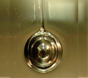
For spheres, a lateral sketch of the symmetry plane is comparable to two-dimensional flow between a circular cylinder and a moving flat plate, as shown in figure 1. However, a perpendicular view through a transparent wall as shown in figures 2(a) and 2(b), reveals a new phenomenon, namely the generation of one or more ‘tracks’ that are shed behind the sphere. In the experiments that led to these figures the plate was replaced by a coated cylinder of large radius rotating about a horizontal axis and the centre of the sphere was stationary inside the cylinder. We can see from figure 2 that the tracks are thin but their depth is greater than that of the incoming film.
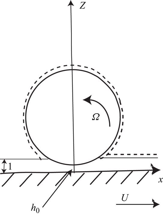
Figure 1. Sketch of the central plane of the sphere showing the non-dimensional parameters; tracks over and behind the sphere are indicated by the dashed lines. The  $x$-axis is vertical.

Figure 2. Two types of steady motion for 14 mm diameter steel spheres on a 0.3 mm layer of silicone oil coating a cylinder of radius 250 mm. (a) A single-track state which only occurs when the sphere is located on the mid-plane of the cylinder. (b) A double-track state, which always occurs when the sphere is located below the mid-plane. The Reynolds number is the same in each case.
In our modelling, we will largely focus on the configuration in figure 2(a), which suggests that the contact region between the sphere and the film is circular. We will see that this can only happen when the sphere is at the point where the cylinder wall is vertical, so that, by symmetry, the net lubrication force normal to the plate is zero. However, when the flow is as in figure 2(b), the shape of the contact region would need to be determined as the solution of a complicated free-boundary problem.
As far as the modelling is concerned, the cylinder will be replaced by a flat plate for most of this paper and the dominant hydrodynamic forces will mostly be assumed to be the lubrication forces calculated from the two-dimensional Reynolds equation that holds within the circle of contact, together with the assumption of atmospheric pressure around this circle. However, we will find that capillary effects are important in some regions. Moreover, as has been discussed briefly in the two-dimensional cases (Mullin et al. Reference Mullin, Ockendon and Ockendon2020; Dalwadi et al. Reference Dalwadi, Cimpeanu, Ockendon, Ockendon and Mullin2021), there exists the possibility of ‘tongues’ of liquid that can exist upstream of the lubricated region and thereby affect the upstream pressure. There are no such tongues in figure 2 but, instead, these images reveal that thin ‘tubes’ of liquid of depth greater than the incoming film inevitably occur around the circle of contact. In figure 2(a), which is typical for small cylinder velocities, the tubes coalesce at the downstream end of the circle, where they give birth to one track returning over the top of the sphere and another continuing upwards on the cylinder. However, as the angular velocity of the cylinder is increased the tubes can detach from the circle before they meet behind the sphere, thereby generating a pair of downstream tracks and corresponding return tracks on the sphere, as in figure 2(b).
We will begin § 2 by considering the purely theoretical problem in which the sphere rotation is to be determined when both the plate velocity and the penetration depth of the sphere are prescribed; such configurations have been considered by Schade & Marshall (Reference Schade and Marshall2011). Then, we will consider what happens when the sphere is free to rotate about its stationary centre, whose position is to be determined, which is the configuration for which figure 2 is relevant. The experiments will be described in more detail in §§ 3 and 4 together with comparisons with the theory for the configuration in figure 2(a).
2. Modelling single-track flows
2.1. Flows with prescribed plate velocity and penetration depth
The simplest configuration is sketched in figure 1 which is a sideways view of the sphere in figure 2(a). The  $x$-axis is taken along the direction of motion of the plate, the $z$-axis is along the normal to the plate through the centre of the sphere and the $y$-axis lies in the plate. The dimensionless film thickness away from the sphere is taken to be $1$ and the sphere rotates about a fixed axis parallel to the $y$-axis. The radius of the sphere is $a$, which is assumed to be large compared with the film thickness $h$. Lengths in the $x, y$ and $z$ directions are non-dimensionalised with respect to $\sqrt {ah}, \sqrt {ah}$ and $h$, respectively, and the velocities in these directions are non-dimensionalised with $U_0, U_0$ and $U_0\sqrt {h/a}$, respectively, where $U_0$ is a typical velocity of the plate along the $x$-axis. The velocity of the plate is $U_0 U$, where the non-dimensional quantity $U$ is prescribed for a particular experiment, and the angular velocity of the sphere is denoted by $U_0\varOmega /a$, where $\varOmega$ is to be determined.
We assume a lubrication flow between the plate and the sphere and non-dimensionalise the pressure deviation from atmospheric with  $\mu U_0 \sqrt {a/h^{3/2}}$, where $\mu$ is the dynamic viscosity of the fluid. Henceforth, $x,y,z$ are non-dimensional variables, $u,v,w$ are the corresponding non-dimensional velocities and $p$ is the non-dimensional pressure.
In these variables, the thickness of the lubrication layer is
 \begin{equation} H=h_0 +\tfrac{1}{2} r^2, \end{equation}
where  $r^2=x^2+y^2$, and the pressure in this region satisfies Reynolds equation
 \begin{equation} \frac{\partial}{\partial x}\left(H^3\frac{\partial p}{\partial x}\right)+\frac{\partial}{\partial y}\left(H^3\frac{\partial p}{\partial y}\right) = 6(U+\varOmega)x.\end{equation}
We now make the a priori assumption that the boundary of the lubrication region is circular with radius  $r_0$, which is suggested by figure 2(a). Also we make the assumption based on the observation in figure 2(a) that the tubes near $r=r_0$ have a thickness of $O(h)$, and hence, from the data in § 3, that the surface tension forces are of $O(10^{-1})$ compared with the lubrication pressure variations. Hence we apply the boundary conditions
 \begin{equation} p=0 \quad \text{on} \ r=r_0=\sqrt{2(1-h_0)}. \end{equation}
The corresponding velocity in the  $x,y$ plane is
 $$\begin{gather} u= \frac{1}{2}z(z-H)\frac{\partial p}{\partial x} + \frac{(\varOmega-U)}{H}z + U, \end{gather}$$
 $$\begin{gather}v= \frac{1}{2}z(z-H)\frac{\partial p}{\partial y}. \end{gather}$$
Separation of the variables in (2.2a) reveals that
 \begin{equation} p=(U+\varOmega)F(r) cos\theta,\end{equation}
where  $\theta$ is a polar angle in the $x,y$ plane measured from the $x$-axis, and Reynolds equation (2.2a) then reduces to
 \begin{equation} r^2\left(h_0+\frac{r^2}{2}\right)\frac{{\rm d}^2{F}}{{\rm d}r^2} + r\left(h_0+\frac{7}{2}r^2\right) \frac{{\rm d}{F}}{{\rm d} r}- \left(h_0 + \frac{r^2}{2}\right){F} = \frac{6r^3}{\left(h_0+\dfrac{r^2}{2}\right)^2},\end{equation}
subject to
 \begin{equation} F(0) = 0 \quad\text{and}\quad {F}(r_0) = 0. \end{equation}
We note that a particular integral of (2.4b) is  $F = -{6r}/{5H^2}$.
The angular velocity  $\varOmega$ and the penetration depth $(1-h_0)$ are related by the condition that there is no moment on the sphere about the axis through its centre, so that
 \begin{equation} \iint_{r < r_0 } \left.\frac{\partial u}{\partial z}\right|_{z=H} \,{{\rm d}\kern 0.06em x} \,{{\rm d}y} = 0.\end{equation}
Equations (2.3a) and (2.4a) imply that that
 \begin{equation} \left.\frac{\partial u}{\partial z}\right|_{z=H} = \frac{H(\varOmega+U)}{2}\left(\frac{{\rm d}F}{{\rm d}r}\cos^2 \theta + \frac{F}{r}\sin^2 \theta \right) +\frac{\varOmega - U}{H}, \end{equation}
and so, after one integration, we see that  $\varOmega$ and $U$ are related by
 \begin{equation} \varOmega\left(\int_{0}^{r_0} r^2F\,{\rm d}r+2\log{h_0}\right) = U\left(-\int_{0}^{r_0} r^2F\,{\rm d}r+2\log{h_0}\right).\end{equation}
 We also note that forces in both the  $x$ and $y$ directions need to be applied at the centre of the sphere in order to maintain equilibrium.
2.2. Tube modelling
We are now in a position to model the flow in the tube of liquid that is observed to flow tangentially around the boundary of the lubricated region. We assume that the pressure in this tube is always small compared with the lubrication pressure variations. We make the further assumption that, in agreement with observation, the lateral dimensions of the tube are greater than, but comparable to, the thickness of the incoming film.
We begin by carrying out a local analysis near the point  $(r_0,\theta )$ for ${\rm \pi} /2<\theta <{\rm \pi}$. From (2.3), the fluid velocity in $r< r_0$ averaged over the depth of the layer is
 $$\begin{gather} \bar{u} = (U+\varOmega)\left(\frac{1}{2}-\frac{1}{12}\left(\frac{{\rm d}F}{{\rm d}r} \cos^2 \theta + \frac{F}{r}\sin^2 \theta \right)\right), \end{gather}$$
 $$\begin{gather}\bar{v} ={-}\frac{(U+\varOmega)}{12}\left(\frac{{\rm d}F}{{\rm d}r} - \frac{F}{r}\right) \sin{\theta} \cos{\theta}. \end{gather}$$
Hence, the averaged velocity components on  $r=r_0$ are equivalent to $(U+\varOmega )/2$ in the $x$-direction in addition to $\frac {1}{12}(U+\varOmega )({{\rm d}F(r_0)}/{{\rm d}r})\cos \theta$ along the radius towards the centre of the sphere. We now let $Q$ be the flux in the tube made non-dimensional with $U_0 h^2$, and perform a mass balance over a small angular change $-\delta \theta$. As shown in figure 3, this leads to
 \begin{equation} \delta Q = U\delta y - \frac{(U+\varOmega)}{2}\delta y+ \frac{(U+\varOmega)}{12}F'(r_0) r_0 \cos{\theta} \delta \theta, \end{equation}
for  ${\rm \pi} /2<\theta <{\rm \pi}$. Thus
 \begin{equation} \frac{{\rm d}Q}{{\rm d}\theta}= \frac{U-\varOmega}{2} r_0 \cos{\theta} + \frac{U+\varOmega}{12}F'(r_0) r_0 \cos{\theta}, \end{equation}
and hence
 \begin{equation} Q=\frac{U-\varOmega}{2} r_0 \sin{\theta} + \frac{U+ \varOmega}{12} F'(r_0) r_0 \sin{\theta} + q_0,\end{equation}
where  $2 q_0$ is the total flux in the track carried over the top of the sphere from the region near $\theta =0$. The quantity $q_0$ can only be determined from an analysis of the three-dimensional Stokes flow in a region near this point. An analogous situation arises in the two-dimensional problem for a cylinder as described in Dalwadi et al. (Reference Dalwadi, Cimpeanu, Ockendon, Ockendon and Mullin2021), in which case the return flow over the cylinder depends on a power of $U$.
$U$.

Figure 3. The flux balance in the tube for  ${\rm \pi} /2<\theta <{\rm \pi}$.
For the region  $0<\theta <{\rm \pi} /2$, we assume that the flux in the tube remains fixed at the value $\frac {1}{2}(U-\varOmega )r_0 + \frac {1}{12}(U+\varOmega )F'(r_0)r_0 + q_0$. Thus, the flux from this tube and its twin in the region ${\rm \pi} <\theta < 2{\rm \pi}$ will create a single track behind the sphere with mass flux $(U-\varOmega )r_0 + \frac {1}{6}(U+\varOmega )F'(r_0)r_0$ together with a single track over the sphere with mass flux $2q_0$.
Although the incoming film ensures that the tube remains close to the sphere for  ${\rm \pi} /2 < \theta < {\rm \pi}$, the only force in the region $0<\theta <{\rm \pi} /2$ that can keep the tube close to the sphere is the radial component of the surface tension force acting on the surface of the tube. As described by Marshall (Reference Marshall2014) for a slightly different thin-film configuration, the dominant surface tension force is that acting on the curved meniscus of length $s$ sketched in figure 4. The $z$-component of this force serves to hold the sphere onto the plate while the other component provides a force along the radius in the $x,y$ plane which acts to keep the tube close to the sphere. It is also shown in Marshall (Reference Marshall2014) that the assumption of a circular meniscus gives an estimate for the force that retains the sphere on the plate which agrees with experiment. Thus we too will assume that the radial force acting on an element of the tube to keep it in place is of order
 \begin{equation} O(Tsr_0\sqrt{a/h}\delta\theta),\end{equation}
where  $T$ is the surface tension.

Figure 4. A cross-section of the tube in a radial plane for  $0<\theta <{\rm \pi} /2$; $s$ and $w$ are dimensional lengths.
If the tube is to remain attached to the sphere for  $0<\theta <{\rm \pi} /2$, the capillary force (2.12) must resist the shear exerted on the tube by the fluid exiting the lubrication region below the tube. Assuming that the amount of fluid entrained into the tube from below is negligible and that the shear force is at most that due to a Couette flow, the outward radial shear force on an element of the tube will be of order
 \begin{equation} O\left(\frac{\mu U_0}{h}(U-\varOmega)\cos{\theta}w\sqrt{ah}r_0 \delta\theta\right) ,\end{equation}
in dimensional terms, where  $w$ is the length indicated in figure 4. Thus, making a comparison with the dominant surface tension force, we see that we need (2.13) to be less than (2.12) when $\theta =0$ to ensure that the tube stays attached to the sphere with a circular wetted region and a single track behind the sphere. If we further assume that both $s$ and $w$ are of $O(h)$, this requires the dimensionless inequality
 \begin{equation} U-\varOmega < O\left(\frac{1}{Ca}\right) , \end{equation}
to hold where the capillary number  $Ca = \mu U_0/T$. We will see in § 2.3 that the relationship between $U$ and $\varOmega$ is approximately linear for the values given in § 4. Hence, from (2.14), we conjecture that a single track will only be possible when $U$ is less than a certain value.
We also note from (2.11) that the amount of fluid in the track behind the sphere will decrease in magnitude as  $U$ decreases, as is observed in the experiments discussed in § 4. We remark further that the tracks generated over and behind the sphere can be considered as free tubes carried along on a rigid base. Their cross-section will still be governed by surface tension forces and visual observation suggests they have a single maximum depth and no vertical tangents.
Experimental evidence concerning the relationship between  $U, \varOmega$ and $h_0$ is only at all easy to obtain when $h_0$ and $\varOmega$ are both selected by the flow and in the next section we will study such a configuration.
2.3. More general steady-state flows
Motivated by the levitation experiments to be discussed in the next section, we now consider the equilibrium configuration for a sphere of mass  $m$ placed inside a rotating coated horizontal cylinder (see figure 5). Assuming the radius of the cylinder is large compared with the radius of the sphere, the flow near the sphere is, to lowest order, the same as that of a sphere near a moving coated flat plate. However, the position of the sphere on the cylinder and the penetration depth are no longer prescribed but depend on the velocity $U$ of the cylinder, which is the control variable. Moreover, the symmetry of the pressure given by (2.4a) ensures that in the single-track configuration there is no force on the sphere normal to the wall and hence the centre of the sphere must lie on the mid-plane of the cylinder.

Figure 5. A schematic diagram of an end view of the apparatus; the variables are all dimensional.
In these circumstances, (2.7) still holds and it is convenient to write it as
 \begin{equation} \left(\varOmega-U\right)\log{h_o} ={-}\frac{(\varOmega + U)}{4}\int_{0}^{r_o} r^2 F(r)\,{\rm d}r, \end{equation}
but it now needs to be coupled to a vertical linear momentum balance. Writing  $M={m g}/{\mu U_0 a}$ where g is the acceleration due to gravity, and remembering that (2.5) holds, we find that
 \begin{align} M ={-}\iint\limits_{r< r_0} x p \,{\rm d}\kern 0.06em x\,{\rm d}y ={-}(U+\varOmega) \iint\limits_{r< r_0} r^2\cos^2\theta F(r) \,{\rm d}r\,{\rm d}\theta ={-}{\rm \pi} (\varOmega+U) \int_{0}^{r_0} r^2 F(r) \,{\rm d}r. \end{align}
When this result is combined with (2.15) we find that
 \begin{equation} M= 4{\rm \pi} (\varOmega- U)\log{h_0} , \end{equation}
and  $\varOmega /U$ can now be considered as a function of $U/M$ by eliminating $h_0$ between (2.15) and (2.17). In order to analyse this problem, it is convenient to introduce a new variable $\lambda$ by writing
 \begin{equation} h_0 = \frac{1}{1+\dfrac{1}{2}{\lambda}^2},\quad F={h_0}^{-{3}/{2}}\hat{F}\quad \text{and} \quad r={h_0}^{1/2}\hat{r} \end{equation}
in (2.4b) so that
 \begin{equation} \hat{r}^2\left(1+\frac{\hat{r}^2}{2}\right)\frac{{\rm d}^2{\hat{F}}}{{\rm d}\hat{r}^2} + \hat{r}\left(1+\frac{7}{2}\hat{r}^2\right)\frac{{\rm d}{\hat{F}}}{{\rm d}\hat{r}}- \left(1 + \frac{\hat{r}^2}{2}\right){\hat{F}} = \frac{6\hat{r}^3}{\left(1+\dfrac{\hat{r}^2}{2}\right)^2}, \end{equation}
subject to
 \begin{equation} {\hat{F}}(0) = 0 \quad \text{and}\quad\hat{F}(\lambda) = 0 . \end{equation}
Then, if we set  $\int _{0}^{r_0} r^2 F(r) \,{\rm d}r= \int _{0}^{\lambda } \hat {r}^2 \hat {F}(\hat {r}) \,{\rm d}\hat {r} = - I(\lambda )$, (2.15) and (2.17) can be rewritten as
 \begin{equation} \frac{\varOmega}{U} = \frac{4\log\left(1+\dfrac{1}{2}{\lambda}^2\right) - I(\lambda)}{4\log\left(1+\dfrac{1}{2}{\lambda}^2\right) + I(\lambda)} \quad \text{and} \quad \frac{2{\rm \pi} U}{M} = \frac{1}{4\log\left(1+\dfrac{1}{2}{\lambda}^2\right)} + \frac{1}{I(\lambda)}. \end{equation}
Thus  $\varOmega /U$ can be found as a function of $U/M$ by eliminating $\lambda$ between these two parametric expressions. This relationship will be compared with the experimental evidence in § 4, but first we will consider it asymptotically for small and large values of $\lambda$.
(i) $\lambda \rightarrow 0$. In this case $\hat {r}$ is $O(\lambda )$ and so, writing $\hat {r}= \lambda R$ and $\hat {F}= \lambda ^3 \bar{F}$, (2.19a) becomes, to lowest order in $\lambda$,
(2.21)with\begin{equation} R^2 \frac{{\rm d}^2 \bar{F}}{{\rm d}R^2}+R\frac{{\rm d}\bar{F}}{{\rm d}R}-\bar{F} = 6R^3 \end{equation}$\bar{F} = 0$ at $R = 0, 1$. Hence
(2.22a,b)and so\begin{equation} \bar{F}= \frac{3}{4}R(R^2 - 1)\quad \text{and} \quad I(\lambda) = \frac{{\lambda}^6}{16} \end{equation}$\varOmega /U \rightarrow 1$ as $U/M \rightarrow \infty$. This is to be expected since the penetration depth is small.
$\lambda \rightarrow 0$. In this case $\hat {r}$ is $O(\lambda )$ and so, writing $\hat {r}= \lambda R$ and $\hat {F}= \lambda ^3 \bar{F}$, (2.19a) becomes, to lowest order in $\lambda$,
(2.21)with\begin{equation} R^2 \frac{{\rm d}^2 \bar{F}}{{\rm d}R^2}+R\frac{{\rm d}\bar{F}}{{\rm d}R}-\bar{F} = 6R^3 \end{equation}$\bar{F} = 0$ at $R = 0, 1$. Hence
(2.22a,b)and so\begin{equation} \bar{F}= \frac{3}{4}R(R^2 - 1)\quad \text{and} \quad I(\lambda) = \frac{{\lambda}^6}{16} \end{equation}$\varOmega /U \rightarrow 1$ as $U/M \rightarrow \infty$. This is to be expected since the penetration depth is small.(ii)
$\lambda \rightarrow \infty$. When we again scale $\hat {r}$ with $\lambda$ and put $\hat {F}= {\lambda }^{-3} \tilde{F}$, (2.19a) now becomes, to the lowest order in $1/\lambda$,
(2.23)with\begin{equation} R^2\frac{{\rm d}^2\tilde{F}}{{\rm d}R^2} + 7R\frac{{\rm d}\tilde{F}}{{\rm d}R} - \tilde{F} = \frac{48}{ R^3}, \end{equation}$\tilde{F}(1) = 0$. Hence
(2.24)which implies that there is a boundary layer when\begin{equation} \tilde{F}={-}\frac{24}{5R^3} + \frac{24}{5}R^{\sqrt{10}-3}, \end{equation}$\hat {r}=O(1)$ such that $\hat {F} \sim -{24}/{5{\hat {r}^3}}$ as $\hat {r} \rightarrow \infty$. Surprisingly, we can find the relevant solution to (2.19a) which is
(2.25)and hence we deduce that\begin{equation} \hat{F}={-}\frac{6\hat{r}}{5\left(1+\dfrac{1}{2}\hat{r}^2\right)^2}, \end{equation}$I(\lambda ) \sim \frac {24}{5}\log {\lambda } + O(1)$. Thus we find that as $\lambda \rightarrow \infty$,
(2.26)This result is also to be expected as\begin{equation} \frac{\varOmega}{U} \sim \frac{1}{4} \quad \text{as} \ \frac{U}{2{\rm \pi} M} \rightarrow 0. \end{equation}$\lambda \rightarrow \infty$ is equivalent to $h_0\rightarrow 0$ and, to the lowest order, the angular velocity of the sphere is the same as if it were fully immersed in liquid.


Numerical solutions for  $\varOmega /U$ as a function of $U/M$ as calculated from (2.20a,b) confirm these observations and will be shown in comparison with experimental results in figure 7(b).
Although our modelling has been confined to configurations with circular wetted regions and a single track, the experiments to be described in the next Section will reveal that twin-track configurations are the norm when the sphere is not on the mid-plane of the cylinder. We also note that, when the small curvature  $K$ of the rotating cylinder is introduced into the model as a regular perturbation, the scenario described above is only changed by $O((Ka)^2)$, with the wetted region becoming slightly elliptical in the vertical direction.
3. The experiment
The experiments were performed in an air-conditioned laboratory where the air temperature was maintained at  $19.0\pm 0.5\,^{\circ }{\rm C}$. The apparatus comprised a precision-machined Plexiglas cylinder with inner diameter $118\pm 0.05$ mm and wall thickness 2 mm. A schematic diagram showing the essential features of the apparatus is given in figure 5. The cylinder was 250 mm long and was held mounted on a pair of precision bearings held in two 50 mm square 70 mm high aluminium posts. The apparatus was mounted on a 10 mm thick machined aluminium base which could be levelled using three adjustable feet. A volume of 25 ml of viscous silicone fluid with measured kinematic viscosity of 13 740 cSt was placed in the cylinder. The cylinder was spun round at 1 Hz for 24 h so that it spread to create a layer of ${\approx }$0.27 mm deep on the inner wall. The experimental conditions were checked in a subsequent investigation using a separate cylinder where a puddle of fluid and an internal scraper was used to set the layer thickness at predetermined values. The results of this investigation are currently being prepared for publication by the third author.
The cylinder was driven using a powerful DC motor which was attached to a pulley on the bearing by a gearbox. The speed of rotation was monitored using a calibrated shaft encoder which produced 400 pulses per revolution. A Nikon  $400$S camera mounted on a tripod was used to capture images and processing was carried out primarily using the software package ImageJ. This was used to measure the position and angular velocity of the spheres. Detailed experiments were performed with precision steel spheres although a wide range of glass and polypropylene spheres were also used to confirm that the general features observed were the same.
4. Overview of observations
The results presented in figure 6 will be used to provide an overview of the main features of the experimental results.

Figure 6. A response diagram for the angular location of equilibrium points for a 19 mm diameter sphere on a 0.3 mm layer of oil.
At small rotation rates of the cylinder, the sphere remains at a fixed location on the rising wall. A graph of the measured angular position plotted as a function of the Reynolds number of the cylinder is presented in figure 6, where  $90^{\circ }$ corresponds to the mid-plane of the cylinder. The equilibrium position of the sphere moves upwards as the speed of the cylinder is increased and the sphere always leaves two tracks behind it as in figure 2(b). The path of equilibrium points is labelled $AB$ in figure 6.
At the point  $B$, the sphere begins to oscillate vertically above and below $90^{\circ }$. When the speed of the cylinder is then reduced, the amplitude of the oscillation decreases until a new steady state is achieved at the point corresponding to the point $C$. At this new steady state the sphere leaves a single track behind it which came as a surprise since, in all experiments on a moving vertical belt, single-track configurations have never been observed. The sphere remains at $90^{\circ }$ as the cylinder speed is reduced, and the track on the cylinder is observed to decrease in size. This continues until the cylinder reaches a speed corresponding to the point $D$. At this point the track behind the sphere disappears and the sphere rolls down the wall back to a lower angle and rapidly adopts a two-track state. Hence both the single- and double-track steady states coexist over the speed range corresponding to $C$ to $D$ in figure 6.
As mentioned above, the sphere rotates steadily at equilibrium locations. The thin lubrication layer is formed between the surface of the sphere and the cylinder wall and a slip speed  ${\omega _b a}/{U_w}=\varOmega /U$ can be measured and compared with the theory in § 2.2. Here, $\omega _b$ is the dimensional angular velocity of the sphere and $U_w$ is the dimensional speed of the wall. A plot of slip speed as a function of the Reynolds number, $Re ={UU_0 h}/{\nu }$, where $\nu$ is kinematic viscosity of the fluid, is given in figure 7(a). Hence, $\varOmega /U$ varies between ${\sim }0.64$ and ${\sim }0.62$ when the sphere is rising up the wall in the two-track state. It then reduces to roughly $0.5$ in the single-track state when the sphere is located at $90^{\circ }$. The apparent gap in the data between $B$ and $C$ corresponds to the range where the motion is oscillatory.

The results between  $C$ and $D$ correspond to the configuration modelled in § 2 and the predictions of (2.20a,b) are shown in comparison with the experimental results in figure 7(b). The experimental results are plotted against $Re$ whereas the dependent variable in (2.20a,b) is $2{\rm \pi} U/M = kRe$ where $k = {2{\rm \pi} \rho {\nu }^2 a}/{mgh}$ and $m$ is 28 g and $\rho$ is the density of the fluid.
Given the number of ad hoc assumptions made during the modelling, the authors believe that the comparison in figure 7(b) is highly satisfactory.
5. Conclusion
A model has been derived for a sphere rotating close to a moving vertical wall coated with a thin viscous fluid layer. This model predicts results for the angular velocity of the sphere which are in good agreement with the single-track observations in figure 7. The model also predicts the flux in the track behind the sphere but experimental confirmation of this quantity is not available.
A more complicated free-boundary problem for the two-track configuration would be needed to describe what happens between the points  $B$ and $C$ in figure 7. Oscillations are observed before the double-track solution collapses into a single-track solution at $C$. Our conjecture is that, once the sphere is on the vertical section of the cylinder wall, the condition (2.14) may hold once the cylinder velocity has decreased sufficiently so that the single-track configuration becomes possible. Although we can only say that the two sides of the inequality (2.14) are of the same order of magnitude between the points $C$ and $D$, it is reassuring that the inequality becomes easier to satisfy as $U$ is decreased.
We also remark that, as the velocity is decreased from  $C$ to $D$, the minimum gap width between the sphere and the cylinder decreases until the theory predicts it is of the order of microns. Thus the boundary conditions for the lubrication model which provides the levitating forces may become invalid.
Single-track configurations have never been observed when the cylinder is replaced by a moving vertical planar belt, and this leads us to conjecture that this is because the curvature of the cylinder allows the sphere to approach its  $90^{\circ }$ equilibrium position very gradually.
Funding
The authors are grateful to Professor P.D. Howell for helpful discussions and to Dr J. Roberts for carrying out the calculations needed for figure 7(b).
Declaration of interests
The authors report no conflict of interest.


 Open access