


1. Introduction
Thermal convections result from the action of a gravity on a fluid endorsing a temperature variation. The natural convection due to the Earth's gravity acting on a stratification of the fluid density, which is temperature-dependent, is a straightforward expression of that statement (see e.g. Schmidt & Milverton Reference Schmidt and Milverton1935; Elder Reference Elder1965; de Vahl Davis & Thomas Reference de Vahl Davis and Thomas1969). However, other mechanisms can be viewed as thermal convection. For instance, the centrifugal acceleration can also act on the stratification of the fluid density to produce the centrifugal buoyancy in a cylindrical annulus (see Walowit, Tsao & DiPrima Reference Walowit, Tsao and DiPrima1964; Busse Reference Busse1970; Meyer, Mutabazi & Yoshikawa Reference Meyer, Mutabazi and Yoshikawa2021). A centrifugal Rayleigh number can be introduced, and its critical value for a rigidly rotating cylindrical annulus is close to that of the classical Rayleigh–Bénard problem (Rayleigh Reference Rayleigh1916), especially for systems with small curvature (see Auer, Busse & Clever Reference Auer, Busse and Clever1995; Kang et al. Reference Kang, Meyer, Yoshikawa and Mutabazi2019). The two previous examples of thermal convection are based on the dependence of the fluid density on the temperature, but other fluid properties that vary with the temperature might lead to a flow that can be characterised as thermal convection. An interesting example is when a non-homogeneous magnetic field is applied to a ferrofluid. As the magnetisation of ferrofluid particles depends on the temperature, the external magnetic field will act on the stratification of magnetic induction (Finlayson Reference Finlayson1970). The Kelvin force then leads to a non-conservative term that is analogue to the Archimedean buoyancy. This can be highlighted by introducing an artificial gravity based on the magnetic properties of the system that would act on the density stratification (see Bozhko & Suslov Reference Bozhko and Suslov2018; Meyer, Hiremath & Mutabazi Reference Meyer, Hiremath and Mutabazi2022). A magnetic Rayleigh number using the magnetic gravity is then introduced in order to characterise the system while keeping in mind the mechanism that brings about the thermal convection of the fluid.
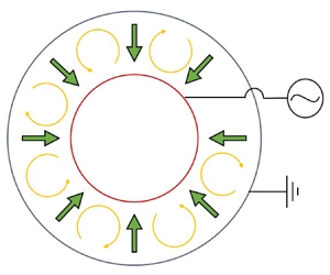
In the present work, a fourth method is used to induce the so-called thermo-electric convection. An external electric field is applied to a dielectric fluid with a stratification of the electric permittivity due to a temperature difference. The restoring force applied to a fluid particle with differential polarisation includes a term that can be seen as the action of a gravity on the density stratification. The thermo-electric convection is investigated in a cylindrical annulus where the inner cylinder is heated and connected to the phase of the electric tension, while the outer cylinder is cooled and electrically grounded (see figure 1). The thermo-electric mechanism can be linked to geophysical or atmospheric flows. Indeed, in a curved channel, the electric gravity provides a central force field that allows for the experimental investigation of planet-like systems (see Chandra & Smylie Reference Chandra and Smylie1972; Yavorskaya, Fomina & Belyaev Reference Yavorskaya, Fomina and Belyaev1984; Zaussinger et al. Reference Zaussinger, Canfield, Froitzheim, Travnikov, Haun, Meier, Meyer, Heintzmann, Driebe and Egbers2019; Travnikov & Egbers Reference Travnikov and Egbers2021). Another application concerns the possibility to enhance the heat transfer between two surfaces (see Turnbull & Melcher Reference Turnbull and Melcher1969; Fogaing et al. Reference Fogaing, Yoshikawa, Crumeyrolle and Mutabazi2014; Jawichian, Siedel & Davoust Reference Jawichian, Siedel and Davoust2023). Dedicated heat exchangers could be based on thermo-electric convection and used in space technologies, where energy saving and apparatus lifetimes are important issues. In both cases, weightlessness is preferred since it eliminates the contribution of non-central force fields and allows the electric gravity to be the only source of convective flows.

Figure 1. Schematic drawing of the cylindrical annulus with applied temperature difference and applied radial electric field, resulting in the central electric gravity field.
When an electric field is applied to a dielectric fluid, the latter undergoes an electro-hydrodynamic force (Landau et al. Reference Landau, Bell, Kearsley, Pitaevskii, Lifshitz and Sykes2013):
 \begin{equation} \boldsymbol{F}_{EHD} = \rho_{e} \boldsymbol{E} - \frac{1}{2}\,\boldsymbol{E}^{2}\,\boldsymbol{\nabla} \varepsilon + \frac{1}{2}\,\boldsymbol{\nabla} \left( \rho\,\frac{\partial \varepsilon}{\partial \rho}\,\boldsymbol{E}^2 \right) . \end{equation}
This force consists of the sum of three terms: the first term on the right-hand side of (1.1) is the electrophoretic force acting on volumes with non-vanishing electric charge density  $\rho _e$; the second term is the dielectrophoretic (DEP) force due to the differential polarisation of dielectric fluid particles; and the last term is the conservative electrostrictive force. The electrophoretic force can be neglected if the applied electric field is alternating with a frequency significantly larger than the inverse of the electric relaxation time $\tau _e = \varepsilon / \sigma _e$ (Jones Reference Jones1979), where $\varepsilon$ is the electric permittivity, and $\sigma _e$ is the electric conductivity of the fluid. As silicone oils with $\tau _e > 200$ s are used as dielectric fluids in the present experiments, a frequency 200 Hz is sufficient to prevent the fluid from building up free charges in its bulk. Additionally, the high frequency of the electric field compared to the inverse of the viscous and thermal dissipation time, both typically 5–400 s for silicone oils (see table 1), allows for the periodic nature of the electric field to be neglected, so its root-mean-square value is considered instead of its periodic value (Turnbull & Melcher Reference Turnbull and Melcher1969). As the electrostrictive force contributes only to the pressure of the confined fluid with static boundaries, the DEP force $\boldsymbol {F}_{DEP}$ is the main contributor to the dynamics of the fluid.
Table 1. Properties and characteristic numbers for silicone oils B3 and B5.

The density  $\rho$ and the electric permittivity $\varepsilon$ are assumed to be linearly dependent on the temperature, i.e. $\rho = \rho _{ref} ( 1 - \alpha \theta )$ and $\varepsilon = \varepsilon _{ref} ( 1 - e \theta )$, where $\alpha$ and $e$ are the thermal expansion coefficient and the coefficient of thermal variation of the permittivity, respectively. The temperature deviation from the reference temperature, $\theta = T - T_{ref}$, is introduced, and the quantities with the subscript ‘ $ref$’ denote the quantity measured at the reference temperature. Under that linear approximation, which is valid as long as the temperature difference applied between the two cylinders is small, the DEP force can be recast as (Yoshikawa, Crumeyrolle & Mutabazi Reference Yoshikawa, Crumeyrolle and Mutabazi2013)
 \begin{equation} \boldsymbol{F}_{DEP} = \boldsymbol{\nabla} \left( \frac{e\,\varepsilon_{ref}\,\theta \boldsymbol{E}^2 }{2} \right) - \rho_{ref}\,\alpha \theta \boldsymbol{g}_e . \end{equation}
The first term on the right-hand side contributes to the pressure balance, and the second term is seen as a thermal buoyancy driven by the electric gravity  $\boldsymbol {g}_e$, written as
 \begin{equation} \boldsymbol{g}_{e} = \frac{e\,\varepsilon_{ref}}{\alpha\,\rho_{ref}}\,\boldsymbol{\nabla} \left( \frac{\boldsymbol{E}^2}{2} \right) . \end{equation}
The direction of the electric gravity depends on the temperature gradient and on the curvature of the annulus. Considering only the case where the inner cylinder is hotter than the outer one, the electric gravity is always centripetal. Analogously to the classical Rayleigh–Bénard problem, as the electric gravity and the temperature gradients are co-directed, there exists a critical temperature difference above which the thermo-electric instability occurs.
The problem of thermo-electric convection in a cylindrical annulus, as presented in figure 1, has attracted attention since the late 1960s, when Smylie (Reference Smylie1966) proposed the idea to use the DEP force to model geophysical fluid dynamics. That idea gave birth six years later to an experimental investigation combined with a linear stability analysis (LSA) by Chandra & Smylie (Reference Chandra and Smylie1972). The critical threshold for the occurrence of thermo-electric convection for a large radius ratio ( $R_1 / R_2 = 0.9$) was calculated, and it was found that the increase of the electric Rayleigh number enhanced the heat transfer rate at the inner cylinder. The thermo-electric coupling through the resolution of the Gauss equation was introduced in the LSA proposed by Takashima (Reference Takashima1980) a few years later. That investigation for axisymmetric modes of instability in a narrow gap has then been extended to the case of non-axisymmetric modes in a gap of arbitrary size by Malik et al. (Reference Malik, Yoshikawa, Crumeyrolle and Mutabazi2012) and by Yoshikawa et al. (Reference Yoshikawa, Crumeyrolle and Mutabazi2013). These investigations highlighted the effect of the curvature on the critical value of the electric Rayleigh number, defined at the mid-gap of the cylinder by
 \begin{equation} L = \frac{\alpha\,\Delta T\,g_e(\bar{r})\,d^3}{\nu\kappa} , \quad \text{with} \ \bar{r} = \frac{R_1 + R_2}{2} , \end{equation}
where  $g_e$ is defined as positive for centripetal electric gravity field $\boldsymbol {g}_{e} = -g_e \boldsymbol {e}_r$ in the cylindrical coordinates $(\boldsymbol {e}_r,\boldsymbol {e}_{\varphi },\boldsymbol {e}_z)$. In particular, it was found that the thermo-electric coupling has a non-negligible effect on the flow stability when the gap between the two cylinders becomes narrow.
Recently, experiments have been carried out under the microgravity ( $\mathrm {\mu }{\rm g}$) condition provided during parabolic flight campaigns (see Meyer et al. Reference Meyer, Jongmanns, Meier, Egbers and Mutabazi2017; Meier et al. Reference Meier, Jongmanns, Meyer, Seelig, Egbers and Mutabazi2018). Visualisations of the flow and of the temperature variation led to the determination of the flow stability after the 22 s of a weightless environment (Szabo et al. Reference Szabo, Meier, Meyer, Barry, Motuz, Mutabazi and Egbers2021). Although the growth of perturbations could be observed, a stationary flow could not be reached, and it was found that the experimental threshold for the destabilisation of the flow was at higher values than the value calculated from a linear stability theory (Yoshikawa et al. Reference Yoshikawa, Crumeyrolle and Mutabazi2013). That difference is mostly attributed to the short duration of $\mathrm {\mu }{\rm g}$ phases provided by the parabolic flight of the ZeroG aeroplane. The result motivated the use of a sounding rocket flight (TEXUS-57). The 6 min of $\mathrm {\mu }{\rm g}$ conditions would then allow the visualisation of the flow destabilisation at parameters close to the theoretical critical value. The analysis of the growth of convection and of the established flow structure can provide fundamental characteristics of the instability that can serve to validate the previously derived linear stability theory, as well as the numerical models. In addition, the destabilisation of the flow at low control parameters would indicate the possibility to produce an optimised thermal system that would be able to transfer heat at lower energy costs.
In the following, the experimental set-up is introduced in § 2, and the applied measurement techniques are described. The linear stability theory is derived in § 3 to provide basic information about the growth of convection close to the onset of instability. The results are shown in § 4. A discussion is given in § 5, and § 6 provides a general conclusion to the work.
2. Experimental set-up
A dielectric fluid is confined between two cylindrical electrodes maintained at different temperatures. The inner cylinder, whose outer surface radius is  $R_1 = 5$ mm, is made of aluminum with a black nickel oxide coating on the outer surface. The inner surface of the outer cylinder has radius $R_2 = 10$ mm. It is made of boron silicate glass, and the inner surface is coated with a transparent conducting oxide, so that the gap is optically free for visualisation techniques through the outer cylindrical surface. Both electrodes have height $H = 100$ mm, which gives aspect ratio $\varGamma = H / (R_2 - R_1) = 20$. The top and bottom lids are made of acrylic glass so the axial direction is optically free. The inner electrode is maintained at temperature $T_1$, and the outer electrode is maintained at temperature $T_2$, so a temperature difference $\Delta T = T_1 - T_2$ between the two surfaces is achieved. In addition, a high alternative electric field is applied with frequency 200 Hz within the dielectric fluid by connecting the inner electrode to the phase of a high-voltage amplifier and by grounding the outer electrode.
As working fluids, silicone oils B3 and B5 are used due to their satisfying dielectric properties (see table 1). In particular, their dielectric constant varies slowly with the applied frequency of the electric field, and internal heating can be neglected since the dissipation factor is low (Yoshikawa et al. Reference Yoshikawa, Kang, Mutabazi, Zaussinger, Haun and Egbers2020). Another advantage is that the silicone oils have a refractive index close to that of acrylic glass, so the reflections and refraction between the transparent materials are limited. Additionally, it was shown that these silicone oils can be used together with a suspension of hollow glass spheres (HGS) to perform particle image velocimetry (PIV) measurements (Adrian & Westerweel Reference Adrian and Westerweel2011). The hollow glass spheres have average radius  $5\ \mathrm {\mu }{\rm m}$ and density $1100\ {\rm kg}\ {\rm m}^{-3}$. They are slightly denser than the silicone oils, so the Earth gravity and the centrifugal acceleration occurring during the acceleration phase of the rocket should lead to the sedimentation of the particles. However, it was shown by Seelig et al. (Reference Seelig, Meyer, Gerstner, Meier, Jongmanns, Baumann, Heuveline and Egbers2019) that the sedimentation velocity of the Potter hollow glass spheres due to the Earth gravity in silicone oil AK5 (with the same properties as B5) was of the order of $10^{-6} {\rm m}\ {\rm s}^{-1}$. During the flight, the gap filling pumps in the mixing loop (see figure 2) are activated just at the beginning of the $\mathrm {\mu }{\rm g}$ phase, which ensures the homogeneous distribution of particles inside the system. Once the system is under weightlessness, no external forces act on the density mismatch between the particles and the fluid. However, the application of the electric field induces the DEP force on the particles, which can result in an electric sedimentation. Indeed, the relative permittivity of the hollow glass spheres is 4.6, which is different from that of the silicone oils. The particles have a larger permittivity than the fluid, and will then tend to be attracted to areas with larger strength in the electric field, i.e. to the inner cylinder. That mechanism is known in biological science since it can be used to separate cells by their permittivity (Pohl & Kaler Reference Pohl and Kaler1979; Zhu, Tzeng & Xuan Reference Zhu, Tzeng and Xuan2010), and one can derive the electric sedimentation of the particle from the DEP force applied to them. Seelig et al. (Reference Seelig, Meyer, Gerstner, Meier, Jongmanns, Baumann, Heuveline and Egbers2019) have estimated that for temperature difference 7 K and peak voltage 7 kV, the electric sedimentation velocity measured at the inner cylinder is $6.3\times 10^{-6}\ {\rm mm}\ {\rm s}^{-1}$. Considering the relatively short duration of the $\mathrm {\mu }{\rm g}$ condition (6 min) and the thermo-electric convective fluid velocity being of the order of $0.1\unicode{x2013}1\ {\rm mm}\ {\rm s}^{-1}$ (see Meier et al. Reference Meier, Jongmanns, Meyer, Seelig, Egbers and Mutabazi2018; Meyer et al. Reference Meyer, Meier, Jongmanns, Seelig, Egbers and Mutabazi2019; Szabo et al. Reference Szabo, Meier, Meyer, Barry, Motuz, Mutabazi and Egbers2021), it is assumed that the sedimentation of the particles can be neglected.

Figure 2. Schematic drawing of the fluid loops for the temperature control and gap mixing.
Two independent fluid loops are used to maintain the temperature difference  $\Delta T$ (see figure 2). The heating fluid flows through the inner cylinder, whereas the cooling fluid flows through a cylindrical tank situated around the outer cylinder. The cooling tank is made of boron silicate glass and is coated with an anti-reflective surface for the use of light-based measurement techniques. The loops have flows of heating and cooling fluids in opposite directions in order to keep the temperature difference constant along the axial direction. The temperature is measured by a set of thermosensors positioned at the inlet and outlet of the experiment cell. Each of the fluid loops is composed of a small fluid reservoir, a pump and a Peltier element that allows for the temperature at the inlet of the cell to be controlled. The chosen fluid in these loops is silicone oil in order to avoid flash-overs that can occur if a leakage allows the cooling or heating fluid to enter inside the gap where the strong electric field is applied.
Additionally to the temperature control, a volumetric flux sensor was placed in the heating loop of the system. Coupling this measurement with those of the temperature at the inlet and at the outlet of the inner cylinder would lead to the rate of heat transfer at the inner cylindrical surface per unit area. The determination of the Nusselt number could then be done by scaling that heat flux with that of the purely conductive one. Unfortunately, an important uncertainty in the temperature measurement combined with a slight increase of the loops’ temperature during the experimental run attributed to a slight drop of pumping efficiency that did not allow the estimation of the Nusselt number to be reliable.
To perform the PIV techniques, the gap is illuminated with a continuous blue (450 nm) laser light sheet in a radial axial plane (see figure 3a). A camera records the motion of the particles inside that plane at 10 frames per second. The radial and axial components of the velocity field  $\boldsymbol {u} = V_r\boldsymbol {e}_r + V_z\boldsymbol {e}_z$ can be measured in the illuminated $(r , z)$ plane. Two mirrors are used in order to achieve a compact system, suitable for fitting in the sounding rocket. Simultaneously, the shadowgraph technique is used to visualise density variations along the azimuthal direction. The gap is lightened along the axial direction with a telecentric homogeneous light illumination of green (520 nm) colour (see figure 3a). Passing through the height of the gap, the light beams are refracted due to temperature variations. The local brightness then changes compared to the original light intensity and is measured at the other side of the cell with a camera equipped with a telecentric objective. The camera is recording the fluid at 5 frames per second. The obtained two-dimensional shadowgraph results from the three-dimensional temperature profile and is used to identify breaking of intensity axial symmetry within the gap. Due to reflections of the light on the hollow glass spheres or on other surfaces, the laser light sheet might be visible on the shadowgraphs, despite the telecentric objective that discriminates most of the rays incoming with a certain incident angle. To limit that cross-contamination of the two visualisation techniques, the illumination by the telecentric system is chosen to be sufficiently large so that the laser light sheet is not visible in the shadowgraphs. In counterpart, a blue filter is equipped on the PIV cameras so only the motion of particles occurring in the laser plane is visible.

Figure 3. Mechanical drawings of (a) an experimental cell with the optics for the measurement techniques, and (b) the TEKUS module equipped with four experimental set-ups as shown in (a) (illustrations courtesy of Airbus Defense and Space).
The complete experiment consists of four identical cylindrical annuli. Each of them has its own fluid loops for control of the temperature differences, and is connected to separated high-voltage amplifiers (see figure 3b). The experimental parameters were chosen so the electric Rayleigh numbers, as defined in (1.4), are higher than the theoretical threshold for the onset of thermo-electric convection, but relatively close to it. In that manner, the growth of the instability is expected to be small, yet positive, for all phases of applied voltage. An overview of the experiment parameters is given in table 2, where the fluid, the applied temperature difference and the applied peak voltage are indicated for each of the cells in their dimensional and dimensionless forms. For each parameter, the duration of the phase of the applied electric field is specified. The value of the electric gravity measured at the mid-gap,  $g_e(\bar {R})$, and that of $L$ are also given. In the cylindrical annulus with radius ratio $\eta = 0.5$, the curvature of the electrodes is the main source of non-homogeneity of the electric field, leading to an electric gravity that is strongly dependent on the applied electric potential, and weakly coupled with the temperature difference between the two surfaces.
Table 2. Experimental parameters in their dimensional and dimensionless forms used during the TEXUS-57 flight, together with the duration  $\Delta t$ of the applied force during the $\mathrm {\mu }{\rm g}$ phase, the intensity of the electric gravity at the mid-gap, and the corresponding value of the electric Rayleigh number.

Before the application of the high voltage, a certain period of time is dedicated to the stabilisation of the conductive state of the flow. During that period, the pump of the filling loop was activated to homogenise the temperature profile within the gap, as well as to distribute uniformly the concentration of particles. After that mixing phase, approximately 30 s is needed for the fluid flow to dissipate and for its temperature profile to establish. Considering the low value of the thermal diffusivity of silicone oils, the temperature is not expected to reach a steady state, but it was shown by Meyer et al. (Reference Meyer, Meier, Jongmanns, Seelig, Egbers and Mutabazi2019) that the growth rate of perturbation is increased when the initial conditions at which the electric field is applied are closer to the conductive state. The first set of high-voltage application lasts for 200 s. The next phase of applied high voltage is performed with higher values of the electric tension. Since it is expected that the growth rate of convective flow gets higher, the duration of the second phase is 80 s shorter than the previous one. With this experimental set-up and the chosen parameters, over the 360 s of available  $\mathrm {\mu }{\rm g}$ conditions, 320 s are used effectively to investigate the dynamic of the dielectric fluids for 8 different values of the electric Rayleigh number.
3. Linear stability theory
Before the results section, the linear stability theory is presented to identify some basic features of the thermo-electric instability and to introduce some predictions from that analysis. The method for the LSA of the problem in a cylindrical annulus has been performed numerous times in different configurations, i.e. in  $\mathrm {\mu }{\rm g}$ conditions (see Malik et al. Reference Malik, Yoshikawa, Crumeyrolle and Mutabazi2012; Yoshikawa et al. Reference Yoshikawa, Crumeyrolle and Mutabazi2013), under Earth gravity conditions (see Meyer et al. Reference Meyer, Jongmanns, Meier, Egbers and Mutabazi2017, Reference Meyer, Crumeyrolle, Mutabazi, Meier, Jongmanns, Renoult, Seelig and Egbers2018), or with the rotation of one or both cylinders (see Yoshikawa et al. Reference Yoshikawa, Meyer, Crumeyrolle and Mutabazi2015; Kang et al. Reference Kang, Meyer, Yoshikawa and Mutabazi2019). We now introduce briefly the main information about linear stability theory, and we refer to the above-mentioned literature for the exhaustive description of the method, and for their tests of validity.
The velocity field  $\boldsymbol {v} = u\boldsymbol {e}_r + v\boldsymbol {e}_{\varphi } + w\boldsymbol {e}_z$ , the temperature deviation from the reference temperature $\theta$, the generalised pressure ${\rm \pi}$, and the electric potential $\phi$ satisfy the continuity equation, the momentum equation, the energy equation and the Gauss law, written as
 $$\begin{gather} \boldsymbol{\nabla} \boldsymbol{\cdot} \boldsymbol{v} = 0 , \end{gather}$$
 $$\begin{gather}\frac{\partial \boldsymbol{v}}{\partial t} + \boldsymbol{v} \boldsymbol{\cdot} \boldsymbol{\nabla} \boldsymbol{v} ={-} \boldsymbol{\nabla} {\rm \pi}+ \nu\,\varDelta \boldsymbol{v} - \alpha \theta \boldsymbol{g}_e , \end{gather}$$
 $$\begin{gather}\frac{\partial \theta}{\partial t} + \boldsymbol{v} \boldsymbol{\cdot} \boldsymbol{\nabla} \theta = \kappa\,\varDelta \theta , \end{gather}$$
 $$\begin{gather}\boldsymbol{\nabla} \boldsymbol{\cdot} \left( \varepsilon\,\boldsymbol{\nabla} \phi \right) = 0 . \end{gather}$$
No-slip boundary conditions are adopted at both cylindrical surfaces, and the temperatures of the inner and outer cylinders are set to  $T_1$ and $T_2$, respectively. Neglecting the periodic nature of the electric tension, the root-mean-square electric potential $V_0 = \sqrt {2}\,V_p / 2$ is applied at the inner cylinder while the outer cylinder is grounded ( $\phi = 0$). The cylindrical annulus is considered to be of infinite length. The set of equations (3.1) and the boundary conditions are non-dimensionalised by scaling the lengths, time, temperature and electric potential by the gap size $d$, the characteristic time of viscous dissipation $d^2 / \nu$, the temperature difference between the two cylinders $\Delta T$, and the effective electric potential $V_0$, respectively. The stability of the flow is studied in the vicinity of the base flow, which is defined as the stationary, axisymmetric and axially invariant solution of the problem. The dimensionless base state is given by
 \begin{equation} \boldsymbol{v}_b = \boldsymbol{0}, \quad \theta_b = \frac{\log \left[r \left(1 - \eta\right) \right]}{\log \eta}, \quad \phi_b = \frac{\log \left(1 - \gamma_e \theta_b \right)}{\log \left( 1 - \gamma_e \right)} . \end{equation}
An infinitesimal perturbation  $( \tilde {u},\tilde {v},\tilde {w},\tilde {{\rm \pi} },\tilde {\theta },\tilde {\phi } )^{\rm T}$ is added to the base state, where the exponent ${\rm T}$ refers to the transpose. The perturbation is then developed into normal modes $\exp [s t + {\rm i} (n \varphi + kz ) ]$ with a complex amplitude $( \hat {u},\hat {v},\hat {w},\hat {{\rm \pi} },\hat {\theta },\hat {\phi } )^{\rm T}$. The parameter $s$ can be complex: $s = \sigma ^* - {\rm i} \omega ^*$, where $\sigma ^*$ is the growth rate of perturbations, and $\omega ^*$ is the propagation frequency. Here, $\sigma ^*$ and $\omega ^*$ are dimensionless, but their dimensional forms $\sigma = \sigma ^*/\tau _{\nu }$ and $\omega = \omega ^*/\tau _{\nu }$ are used later for a direct connection to the experiment. The orientation and size of the mode is determined by the azimuthal mode number $n$ and the axial wavenumber $k$. The dimensionless set of equations for the amplitude of perturbations reads
 $$\begin{gather} 0 = \left( \frac{{\rm d}}{{\rm d} r} + \frac{1}{r} \right) \hat{u} + \frac{{\rm i}n}{r}\,\hat{v} + {\rm i}k\hat{w} , \end{gather}$$
 $$\begin{gather}s\hat{u} = \varDelta \hat{u} - \frac{{\rm d} \hat{\rm \pi}}{{\rm d} r} - \frac{\hat{u}}{r^{2}} - \frac{2 {\rm i} n}{r^{2}}\,\hat{v} - \frac{\gamma_e V_E^2}{Pr} \left( g_{e,b} \hat{\theta} + \hat{g}_{e,r} \theta_b \right) , \end{gather}$$
 $$\begin{gather}s \hat{v} = \varDelta \hat{v} - \frac{{\rm i} n}{r}\,\hat{\rm \pi} - \frac{\hat{v}}{r^2} + \frac{2 {\rm i} n}{r^2} \hat{u} - \frac{\gamma_e V_E^2}{Pr}\,\theta_b \hat{g}_{e,\varphi} , \end{gather}$$
 $$\begin{gather}s \hat{w} = \varDelta \hat{w} - {\rm i} k \hat{\rm \pi} - \frac{\gamma_e V_E^2}{Pr}\,\theta_b \hat{g}_{e,z} , \end{gather}$$
 $$\begin{gather}s \hat{\theta} = \frac{1}{Pr}\,\varDelta \hat{\theta} - \frac{{\rm d} \theta_b}{{\rm d} r}\,\hat{u} , \end{gather}$$
 $$\begin{gather}0 = \left(1 - \gamma_e \theta_b \right) \varDelta \hat{\phi} - \gamma_e\,\frac{{\rm d} \theta_b}{{\rm d} r}\, \frac{{\rm d} \hat{\phi}}{{\rm d} r} - \gamma_e\,\frac{{\rm d} \phi_b}{{\rm d} r} \left( \frac{{\rm d}}{{\rm d} r} + \frac{1}{r} \right) \hat{\theta} - \gamma_e\,\frac{{\rm d}^2 \phi_b}{{\rm d} r^2}\,\hat{\theta} , \end{gather}$$
where the Laplacian operator  $\varDelta$ reads
 \begin{equation} \varDelta = \frac{1}{r}\,\frac{{\rm d}}{{\rm d} r} \left( r\,\frac{{\rm d}}{{\rm d} r} \right) - \frac{n^2}{r^2} - k^2 . \end{equation}
The dimensionless electric potential  $V_E = V_p / \sqrt {2}\,V_{f}$ and the thermo-electric parameter $\gamma _e = e\,\Delta T$ have been introduced, where $V_f = ( \rho _{ref}\,\kappa \nu / \varepsilon _{ref} )^{1/2}$ is the characteristic voltage for a given fluid. The base electric gravity is given by $g_{e,b}= \boldsymbol {\nabla } ( \boldsymbol {\nabla } \phi _b )^2$. The amplitude of all perturbations vanishes at the cylindrical surfaces $\hat {u} = \hat {v} = \hat {w} = \hat {\theta } = \hat {\phi } = 0$. The momentum equations (3.3b)–(3.3d) include the perturbation of the electric gravity along the three spatial components:
 \begin{equation} \hat{g}_{e,r} = \frac{{\rm d} \phi_b}{{\rm d} r}\,\frac{{\rm d}^2 \hat{\phi}}{{\rm d} r^2} + \frac{{\rm d}^2 \hat{\phi}_b}{{\rm d}r^2}\,\frac{{\rm d} \hat{\phi}}{d r}, \quad \hat{g}_{e,\varphi} = \frac{{\rm i}n}{r}\,\frac{{\rm d} \phi_b}{{\rm d} r}\, \frac{{\rm d}\hat{\phi}}{{\rm d} r}, \quad \hat{g}_{e,z} = {\rm i}k\,\frac{{\rm d} \phi_b}{{\rm d} r}\, \frac{{\rm d} \hat{\phi}}{{\rm d}r} . \end{equation}
The system of (3.3) is solved using a spectral collocation method as described in Yoshikawa et al. (Reference Yoshikawa, Crumeyrolle and Mutabazi2013), with the order of the Chebyshev polynomial as 30 to ensure the convergence of calculations.
The growth rate is determined for fixed values of the control parameters  $(\eta, Pr , \zeta, \gamma _e , V_E )$, and for various values of $k$ and $n$. The global maximum of the growth rate determines the most critical modes for the given set of parameters, and the state for which the maximum value coincides with $\sigma ^* = 0$ corresponds to the critical state $(V_{E,c}, k_c, n_c, \omega ^*_c)$. Figure 4 shows the evolution of the growth rate in dimensional form as a function of the axial wavenumber $k$ for various control parameters. For $\gamma _e = 0.0053$, the critical state is obtained for $V_{E,c} = 673$, $k_c = 1.528$ and $n_c = 4$. The growth rate of the most critical state is also shown for the different control parameters applied to the silicone oil B5 during the TEXUS-57 flight. The growth rate increases with increasing $V_E$ and $\gamma _e$, i.e. with increasing $L$. The number of modes in the azimuthal direction increases with $L$, from $n=4$ at the critical state, to $n=6$ for the highest value of $L$ applied to the liquid. All the determined modes are stationary ( $\omega ^* = 0$) and helical ( $n \neq 0$ and $k \neq 0$). In Yoshikawa et al. (Reference Yoshikawa, Crumeyrolle and Mutabazi2013), it is demonstrated that the critical state of the flow is independent of the Prandtl number. Another important result is that when the radius ratio is not too large, the critical values of $L_c$, $k_c$ and $n_c$ are independent of the temperature difference between the two cylinders. In the special case $\eta = 0.5$, the critical Rayleigh number is $L=1498$.

Figure 4. Dimensional growth rate  $\sigma$ of the most critical mode as a function of the axial wave number for silicone oil B5 and for various control parameters.
4. Experimental results
As seen in table 2, the electric Rayleigh number takes values from  $L = 2774$ to $L = 9227$ in the present experiment. It corresponds to 1.85 and 6.17 times the critical value $L_c = 1498$ determined by Yoshikawa et al. (Reference Yoshikawa, Crumeyrolle and Mutabazi2013). For silicone oil B5 in the cylindrical annulus with the same dimension as for the present experiment, the minimum value of $L$ for which an instability has been observed during the weightless environment of a parabolic flight was $L = 3995$. Under the Earth gravity, Seelig et al. (Reference Seelig, Meyer, Gerstner, Meier, Jongmanns, Baumann, Heuveline and Egbers2019) conducted an experiment for a vertical cylindrical annulus with the same dimensions and with the same dielectric liquid (silicone oil AK5). For temperature differences 5 and 10 K, thermo-electric instabilities were detected for $V_E \approx 1020$ at the lowest. During the $\mathrm {\mu }{\rm g}$ condition of the TEXUS flight, the PIV and the shadowgraph techniques highlighted the growth of a thermo-electric instability for all investigated values of $L$.
$L$.
The results from the PIV techniques are shown in figure 5 for all investigated values of  $L$ at the end of their respective phase of active high voltage. The plots indicate the velocity field and the isosurface of the azimuthal component of the vorticity $\omega _{\varphi } = \partial V_z / \partial r - \partial V_r / \partial z$ measured in the $(r,z)$ plane where the laser light sheet is illuminating the particles. The velocity field clearly indicates the occurrence of thermo-electric convection for all values of $L$. For $L = 2774$, counter-rotating pairs of vortices are observed only in the vicinity of the lids. Between $z = 10$ mm and $z = 70$ mm, the flow is mainly radially outwards, indicating a sheet-like convective flow, therefore $V_z$ and $\omega _{\varphi }$ are small in that area. For higher values of $L$, the counter-rotating vortices are more pronounced and extend along the whole height of the gap. For all values of $L$, the flow intensity seems to be increasing continuously with the increase of $L$. Numerical simulations were performed by Kang & Mutabazi (Reference Kang and Mutabazi2021) for $L = 6246$ in the case of weightlessness. They predicted helical modes with 5–6 pairs of vortices along the axial direction, and amplitude of the azimuthal vorticity approximately $\omega _{\varphi } = 0.2\ {\rm s}^{-1}$. Their results are in good qualitative agreement with the present experimental ones. The number of modes along the axial direction seems higher in the experiments, which could explain why the numerical result slightly underestimates the amplitude of the $\omega _{\varphi }$.

Figure 5. Velocity field and surface of isovalues of the azimuthal component of the vorticity at the end of the phase of high-voltage application for (a)  $L = 2774$, (b) $L = 2933$, (c) $L = 3995$, (d) $L = 4583$, (e) $L = 5586$, ( f) $L = 5905$, (g) $L = 8044$ and (h) $L = 9227$.
The shadowgraphs corresponding to the different values of  $L$ are shown in figure 6. To obtain those shadowgraphs, the grey level of a given image is normalised with that of a reference image. That reference corresponds to the case when no temperature difference and no electric tension are applied. The value of the local light intensity $I$ is $I = 1$ when the local grey level is equal to that of the reference case. For all values of $L$, the light intensity profiles overcome a break of symmetry along the azimuthal direction, indicating the occurrence of the thermo-electric instability. For values up to $L = 3995$ of the electric Rayleigh number, the light intensity is slightly larger around the mid-gap. This higher intensity has a certain extension along the azimuthal direction where the non-homogeneity of the light intensity is slightly visible. For larger values of $L$, the non-axisymmetric behaviour of the light intensity profile is clearly visible. The light intensity measured by shadowgraphy highlights the formation of hot and cold jets at different azimuthal positions that, combined with the previous results of PIV along the axial direction, indicates that the thermo-electric instability tends to have a helical structure, as predicted by Malik et al. (Reference Malik, Yoshikawa, Crumeyrolle and Mutabazi2012). For all parameters, the pattern observed in the shadowgraph is stationary. At least for a given fluid, the light intensity variations increase with increasing $L$; however, it seems that the silicone oil B3 is more sensitive to the shadowgraph technique than the silicone oil B5, so that the light intensities seem globally higher for B3 at equivalent values of $L$. Small differences in refractive index, or its variation rate with respect to the density, might explain such an observation. Although the shadowgraphs indicate the break of symmetry of the flow along the azimuthal direction, the technique does not allow a clear determination of the mode number. The main difficulty comes from the fact that the measurement is performed along a large fluid distance, which prevents the proper tracking of the jets along the axial direction.

Figure 6. Shadowgraphs at the end of the phase of high-voltage application for (a)  $L = 2774$, (b) $L = 2933$, (c) $L = 3995$, (d) $L = 4583$, (e) $L = 5586$, ( f) $L = 5905$, (g) $L = 8044$ and (h) $L = 9227$.
The time evolution of the velocity field and of the light intensity profiles can be analysed through the use of space–time diagrams. The radial velocity is measured at the mid-gap along the axial direction, and the light intensity is measured at the mid-gap along the azimuthal direction. The time variations of those measurements are shown in figure 7 for two values of  $L$. The temporal evolution of the radial velocity highlights the growth of the convective pattern starting from the lids of the cylindrical annulus for electric Rayleigh numbers up to $L = 3995$ (see figures 7a,c). This perturbation then brings about the convection at the mid-height of the cylinders. This mechanism seems to be in good agreement with the numerical simulation conducted by Gerstner (Reference Gerstner2020), who described the growth of toroidal vortices close to the boundaries. The growth of these axisymmetric modes then propagates progressively towards the mid-height of the cell, at which point the modes become non-axisymmetric. For larger values of $L$, the thermo-electric convection grows from the lids as well as from the bulk of the cells. The space–time diagrams for both the radial velocity and the light intensity show that the general amplitude of the perturbations reaches saturation, and that the instability is stationary. However, the modes seem to be still slowly evolving at the end of the phase of applied high voltage for some values of $L$. For instance, for $L = 9227$ (see figures 7b,d) the space–time diagram of $V_r$ indicates that some outward jets (positive radial velocity) are being split in two whilst some inward jets (negative radial velocity) are merging. The space–time diagram for the light intensity at the same value of $L$ is also indicating a certain modification of the shape of the modes. This behaviour is observed for different values of $L$ and seems to indicate that the three-dimensional convective cells are taking a long time to adapt to their available space and to reach a steady state, or that they might not be able to do so.

Figure 7. Space–time diagrams of (a,b) the radial component of the velocity along the axial direction and (c,d) the light intensity along the azimuthal direction. Both quantities are measured at the mid-gap for (a,c)  $L = 2933$ and (b,d) $L = 9227$. The origin of the time is taken at the instant when the high voltage is applied.
In an analogous problem, Odenbach (Reference Odenbach1995) used the amplitude of the perturbation of temperature to determine the critical value of the magnetic Rayleigh number. For his investigation, a magnetic field was applied to a ferrofluid during the  $\mathrm {\mu }{\rm g}$ phase of a sounding rocket flight. The extrapolation method used to evaluate the critical control parameter relies on the dynamic of the formation of coherent structures in media. The nonlinear Ginzburg–Landau equation describes weakly nonlinear spatio-temporal phenomena in the vicinity of the primary bifurcation. For a stationary and periodic instability, as is the case here, the equation can be written as (Cross & Hohenberg Reference Cross and Hohenberg1993; Manneville Reference Manneville2005)
 \begin{equation} \tau_0\,\frac{\partial A}{\partial t} = \delta A + \xi_0^2\,\frac{\partial^2 A}{\partial z^2} - l\,|A|^2\,A , \end{equation}
where  $A$ is the amplitude of a perturbation mode, and $\tau _0$ and $\xi _0$ are the characteristic time and the coherent length of a perturbation, respectively. These quantities that correspond to linear mechanisms are scales for the variation of a perturbation in time and in space. The Landau constant $l$ originates from a nonlinear mechanism that leads to the saturation of the mode amplitude when it is positive (super-critical bifurcation). The reduced control parameter $\delta = ( L - L_c ) / L_c$ indicates the proximity to the critical threshold and should not be too high, so that (4.1) is valid.
During the TEXUS-57 flight, all the studied control parameters are above the critical values, and an unstable regime was observed systematically. Indeed, it was a choice not to investigate parameters that would allegedly result in a purely conductive state. The distinction between the conductive base state when  $L < L_c$ and the unstable regime when $L > L_c$ was, however, determined experimentally by Seelig et al. (Reference Seelig, Meyer, Gerstner, Meier, Jongmanns, Baumann, Heuveline and Egbers2019) under the influence of a vertical gravity field, and it was also investigated through numerical simulations and LSA when considering $\mathrm {\mu }{\rm g}$ conditions. We therefore assume the supercriticality of the bifurcation and admit that conveniently, (4.1) describes the dynamics of the amplitude of the modes of instability.
The norm of the radial component of the velocity at a given radial position is averaged over the height of the cavity and used to evaluate the amplitude of the modes, so that
 \begin{equation} A = \frac{1}{H}\int_0^H |V_r| \,{\rm d}z. \end{equation}
By making this choice, the variation of the amplitude close to a solid boundary is hidden and the second term on the right-hand side of (4.1) should be cancelled. Indeed, the mode structure is three-dimensional, so it is not relevant to evaluate the local amplitude envelope at a single azimuthal angle, since it was shown that the modes also have a certain periodicity in the azimuthal direction. The amplitude  $A$ measured at the mig-gap is plotted over time in figure 8 for various values of the electric Rayleigh number during the first 120 s of the phase of applied voltage. For each of the values of $L$, the amplitude of the modes initially increases exponentially with a constant growth. After a sufficiently long time, the amplitude saturates to a constant value $A_s$, which depends on $L$. For sufficiently large values of $L$, at the transition from constant growth to saturation, the amplitude overshoots its saturation value and may start to oscillate around the value $A_s$. One can see that the higher the electric Rayleigh number, the higher the growth rate of the mode during the linear growth of the perturbation amplitude.

Figure 8. Evolution of the amplitude of perturbation  $A$ at the mig-gap as defined in (4.2) as a function of time for different values of $L$. The initial time is synchronised with the beginning of the high-voltage application phase.
When a perturbation mode saturates, its amplitude becomes stationary and (4.1) reduces to  $|A|^2 = \delta / l$, which indicates a proportionality between the square of the amplitude and the electric Rayleigh number. That mechanism is observed in numerous problems of pattern formation in fluid mechanics (Odenbach Reference Odenbach1995; Le Gal et al. Reference Le Gal, Harlander, Borcia, Le Dizès, Chen and Favier2021). The evolution of $A_{s}^2$ with $L$ is shown in figure 9. For two values of the electric Rayleigh number, i.e. $L = 5586$ and $L = 8044$, the value of $A$ did not converge to a constant so that $A_s$ could not be extracted in those cases. For all other values of $L$, the time evolution of the amplitude $A$ is evaluated at a fixed radius corresponding to the mid-gap $\bar {R}$, as well as at the neighbouring radial positions $R \pm {\rm d}r$, with ${\rm d}r = 0.2$ mm. The last 10 s of the phases of applied electric field are used for each radius to generate reliable statistics data, from which the average provides the value $A_s$, and the standard deviation gives the error bar that takes into account uncertainties in the velocity and in the positioning of the mid-gap. A linear fit between the square of the amplitude $A_s$ of the modes and the electric Rayleigh number is given, and its extrapolation at $A_{s}^2 = 0$ provides the critical value $L_c = 1628$ for the electric Rayleigh number. This value is to be compared with the value of $L_c = 1498$ derived from LSA in Yoshikawa et al. (Reference Yoshikawa, Crumeyrolle and Mutabazi2013) and from numerical simulations in Travnikov, Crumeyrolle & Mutabazi (Reference Travnikov, Crumeyrolle and Mutabazi2015) for any values of the Prandtl number and for a radius ratio $\eta = R_1/R_2 = 0.5$. The error in the prediction made by the linear interpolation is approximately $L_c \pm 220$, which corresponds to a 15 % accuracy in the determination of the critical parameter. Using the critical value determined above, i.e. $L_c = 1628$, the calculation of the slope of the linear fit with respect to the parameter $\delta$ provides an experimental value for the Landau constant $l = ( \partial |A_s|^2 / \partial \delta )^{-1} = 97.22\ {\rm s}^2\ {\rm mm}^{-2}$.

Figure 9. Evolution of the square of the saturated amplitude as a function of the electric Rayleigh number.
Another method to derive the critical value of  $L$ is to study the growth of the perturbation amplitude $A$ (see Yoshikawa & Wesfreid Reference Yoshikawa and Wesfreid2011). For small amplitudes far from the solid boundaries, (4.1) implies an exponential evolution of $A$ with time. Writing the perturbation amplitude as $A(r,\varphi,t) = A_{0}(r,\varphi )\exp (\sigma t)$, where $\sigma$ is the growth rate of the perturbation, (4.1) leads to $\sigma = \delta /\tau _0$. That latest result indicates that when the perturbation starts to grow, the growth rate of $A$ is proportional to the electric Rayleigh number. To determine the growth rate $\sigma$, a certain interval of time is chosen so that the evolution of $A$ satisfies an exponential growth. The slope of the curve $\log (A) = f(t)$ within the selected interval corresponds to the growth rate $\sigma$. The growth rate is determined through the evolution of the amplitude measured at various radial positions in the interval $r \in [6.5, 8.5]$ mm, where $A$ is evaluated with sufficient accuracy. The interval choice for the estimation of the linear growth is also varied slightly so the resulting error is taken into account.
The variations of  $\sigma$ as functions of the electric Rayleigh number are shown in figure 10. The growth rate is zero at the onset of thermo-electric convection, i.e. at $L = L_c$, and increases linearly with $L$ for relatively small values of $L$. A linear fit is applied as a function of $L$ for $L < 6500$, so that the nonlinear term in (4.1) can be neglected. Using that fit to determine the critical value of the electric Rayleigh number, the evolution of $\sigma$ gave the value $L_c = 1695 \pm 400$. However, the two methods gave similar values of the critical parameter, and the difficulty of fitting efficiently an exponential growth to the evolution of $A$ brings about a critical electric Rayleigh number with approximately 25 % accuracy. Using the determined value $L_c = 1695$, the evaluation of the slope of $\sigma$ as a function of $L$ provides an experimental value for the coherent time $\tau _0 = ( \partial \sigma / \partial \delta )^{-1} = 13.37$ s. Figure 10 also shows the evolution of the growth rate obtained from LSA for silicone oils B3 and B5 by fixing all parameters to those of the critical state, except for $V_E$, whose variation induces the variation of $L$. The two curves are linear and cross the line $\sigma = 0\ {\rm s}^{-1}$ at $L = 1498$. The value of $\sigma$ for $L > 1498$ depends slightly on the fluid viscosity, and its dependence on $\gamma _e$ can be neglected. There is a qualitative agreement between the results from LSA and the experimental ones, and the characteristic times $\tau _0$ derived from LSA are $\tau _0 = 16.2$ s for B5, and $\tau _0 = 16.7$ s for B3. These values are in relatively good agreement with the experimental results.

Figure 10. Evolution of the growth rates of  $A$ as functions of the electric Rayleigh number. The results from LSA are also shown for the two different fluids with $k = k_c = 1.528$ and $n = n_c = 4$.
Multiplying (4.1) with the amplitude and neglecting the end effect by suppressing the spatial derivative of the amplitude, we obtain the Stuart–Landau equation (Stuart Reference Stuart1960):
 \begin{equation} \frac{\partial |A|^2}{\partial t} = \frac{2 \delta}{\tau_0}\,|A|^2 - \frac{2 l}{\tau_0}\,|A|^4. \end{equation}
This equation admits a solution written in the form (Landau & Lifshitz Reference Landau and Lifshitz2013; Drazin & Reid Reference Drazin and Reid2004)
 \begin{equation} |A(t)|^{{-}2} = \frac{l}{\delta} + \left( |A_0|^{{-}2} - \frac{l}{\delta} \right) \exp \left( - 2 \delta\,\frac{t}{\tau_0} \right) , \end{equation}
where  $A_0 = A(t=0)$ is the amplitude at the initial time. The parameter $\delta$ is based on the critical electric Rayleigh number extracted from the saturated amplitude evaluation, i.e. $L_c = 1628$. Using the values of the Landau constant $l$ and the characteristic time $\tau _0$ determined experimentally, we can plot the evolution of the amplitude and compare it with the experimental one. The comparison is shown in figure 11 for various values of $L$. For each of the curves, the initial value of the modes’ amplitude $A_0$ is selected so that the analytically determined curve fits the experimental one the best. The exponential growth in time of the amplitude derived from (4.4) is in quantitative good agreement with the experimental observation. The agreement is still valid for $L = 9227$, for which the growth rate $\sigma$ was found to have an offset compared to the linear extrapolation derived in figure 10. For some given values of $L$, the saturated amplitude $A_s$ determined experimentally might differ from the asymptotic values $A(t \rightarrow \infty ) = \sqrt {\delta /l}$, but the error exhibited a maximum of 15 %. It is found experimentally that for sufficiently large values of $L$, the amplitude overshoots its saturated value and starts to oscillate around the equilibrium state. The solution of the Stuart–Landau equation does not include that mechanism, and higher-order terms would be required in (4.3). Overall, the good agreement justifies the use of the Stuart–Landau equation to characterise the amplitude evolution, and to validate the use of a constant growth rate for the determination of the experimental data shown in figure 10.

Figure 11. Comparison of the amplitude evolution measured experimentally and calculated analytically from (4.4).
5. Discussion
The duration of  $\mathrm {\mu }{\rm g}$ conditions is an important parameter for our experiments. For high values of the electric Rayleigh number, parabolic flight campaigns play an important role since the destabilisation of the flow can be observed and analysed. But if a fully established flow is required, or if relatively small values of $L$ are investigated, then the 22 s of $\mathrm {\mu }{\rm g}$ offered by parabolic flights is not sufficient, and long-term weightlessness would be necessary. The space–time diagrams given in figure 7 indicate that for the considered values of $L$, 50–100 s of applied DEP force is needed to have a relatively well-established convective flow. From (4.4), one can derive the time $t_s$ needed for the instability mode to reach 99 % of the saturation value $\sqrt {\delta /l}$. Remarking that the initial amplitude of the mode verifies $A_0 \ll 1$, the time $t_s$ reads
 \begin{equation} t_s \approx \frac{\tau_0}{2 \delta} \left\lbrace \log \left[ \frac{A_0^{{-}2} \left( \delta / l \right)}{0.99^{{-}2} -1} \right] + A_0^2\,\frac{l}{\delta} - \epsilon ( A_0^4 ) \right\rbrace , \end{equation}
where  $\epsilon$ is in the fourth order of the initial amplitude and can therefore be neglected. The saturation time is infinite when $\delta \rightarrow 0$ through positive values, and it tends to zero for large $\delta$. From (5.1), it is possible to determine the required value of $L$ to reach a saturated state within a given time. Table 3 indicates some values of $L$ corresponding to various saturation times and for two different values of $A_0$ that correspond to the order of magnitude of noise when measuring the velocity (in ${\rm mm}\ {\rm s}^{-1}$). If a saturated state is desired for an experiment under $\mathrm {\mu }{\rm g}$ conditions, then the strength of the DEP force must be adjusted accordingly. For example, the drop-tower from the ZARM institute in Bremen provides $\mathrm {\mu }{\rm g}$ phase 9.5 s (Von Kampen, Kaczmarczik & Rath Reference Von Kampen, Kaczmarczik and Rath2006), which would require an electric Rayleigh number larger than 13 000. Such a value of $L$ corresponds to a peak voltage of the order of 10 $^4$ for a silicone oil B5 with temperature difference 5 K. Similarly, the 22 s of $\mathrm {\mu }{\rm g}$ conditions would need a minimum of 7000 V to reach a saturated state. Although these electric potentials are achievable, they are accompanied with technical difficulties, and safety issues. Depending on the desired observation, and on the technical limits, the present results might serve as a guide to select the control parameters.
Table 3. Electric Rayleigh numbers necessary for a given saturation time.

Since 2013, the participation in ten parabolic flight campaigns allowed for the collection of data under  $\mathrm {\mu }{\rm g}$ conditions, where experiments on thermo-electric convection were performed in various geometries, with various fluids, and with different measurement techniques. In six of these campaigns, a silicone oil B5 was used in a cylindrical cavity with characteristics corresponding to those described in § 2. For these experiments, the break of symmetry of the shadowgraphs’ light intensity along the azimuthal direction, and the growth of a flow measured by PIV, led to the determination of the flow stability after 22 s of weightlessness (see Meier et al. Reference Meier, Jongmanns, Meyer, Seelig, Egbers and Mutabazi2018; Jongmanns Reference Jongmanns2019). Out of 64 different parameters, an experimental stability diagram is determined and shown in figure 12. The diagram is spanned by the dimensionless electric potential $V_E$ and the thermo-electric parameter $\gamma _e$. The blue diamonds indicate flow where no perturbation was detected during the 22 s of $\mathrm {\mu }{\rm g}$ phase. The red circles show parameters where either a break of symmetry along the azimuthal direction was observed by shadowgraphy, or a flow measured by PIV started to grow, or both, during the 22 s of $\mathrm {\mu }{\rm g}$ The isovalues of the growth rate of the most critical state determined with linear stability theory derived in § 3 are also shown as a comparison. The line with growth rate $\sigma = 0.1\ {\rm s}^{-1}$ follows quite well the experimental threshold between stable and unstable flow until $\gamma _e = 0.005$. At larger $\gamma _e$, the experimental threshold corresponds to values of $\sigma$ that increase with $\gamma _e$. Due to the limited duration of the $\mathrm {\mu }{\rm g}$ phase during parabolic flights, it is expected that the threshold obtained with the linear stability for $\sigma = 0$ does not coincide with the experimental observation. However, the experiment threshold follows qualitatively the isovalues of $\sigma$. The deviation observed above a certain temperature difference can be attributed to two main sources. The first could be the non-validity of the linear approximation made to model the variation of the electric permittivity with the temperature. That non-validity might lead to a stabilisation of the flow with respect to the linear model that would explain the observation. A second reason could be the enhanced thermal convection occurring at higher temperature differences, and in particular during the hyper-gravity phase happening just before the beginning of the $\mathrm {\mu } {\rm g}$ phase in a parabolic flight. The initial flow might play a stabilising role, since the strength of the DEP force has to overcome the higher inertia of the fluid.

Figure 12. Stability diagram for silicone oil B5 spanned by the dimensionless electric potential  $V_E$ and the thermo-electric parameter $\gamma _e$. The blue diamonds and the red circles indicate the flow stability after the 22 s of the $\mathrm {\mu }{\rm g}$ provided during parabolic flight campaigns (PFC). The blue diamonds indicate the parameters for which no instability was found, whereas the red circles indicate the parameters where thermo-electric instabilities were observed. The black crosses show the results from the sounding rocket flight, which were all corresponding to unstable flows. The contour plot shows isovalues of the growth rate calculated from the linear stability theory.
The four experimental parameters investigated for silicone oil B5 during the sounding rocket are added to the stability diagram with large circles. The longer time under  $\mathrm {\mu }{\rm g}$ allows the observation of the flow destabilisation for parameters that did not indicate the occurrence of instability at the end of the $\mathrm {\mu }{\rm g}$ phase of a parabolic flight, or during laboratory experiments. Results of parabolic flight experiments with silicone oil B3 are lacking at the moment so we could not provide a similar stability diagram; however, we expect the conclusion to be the same as that for silicone oil B5.
6. Conclusion
An experiment on the stability of dielectric fluid in a cylindrical annulus under the influence of a radial DEP force was performed during the TEXUS-57 sounding rocket flight, providing 6 min of microgravity ( $\mathrm {\mu }{\rm g}$) conditions. Four identical experimental cells housed two different fluids and imposed two temperature differences between the cylinders. Additionally, two different values of electric potential were applied on each cell so a total of eight values of the electric Rayleigh number were investigated, from $L = 2774$ to $L = 9227$. The PIV techniques allowed the determination of the flow velocity in a section co-planar with the cylinders axis, and the shadowgraph technique gave information on the break of axisymmetry of the fluid density along the azimuthal direction. For all values of $L$, the conductive state of the dielectric fluids destabilised, and thermo-electric convection occurred with an amplitude that increased with the increase of $L$. The analysis of the growth rate of the radial velocity and of its amplitude helped in the determination of the experimental critical electric Rayleigh number, which is found to be satisfyingly close to the theoretical value $L_c = 1498$. The time needed to reach a stationary state is large. Even after 200 s of applied electric field, it was found that the fluid is still adapting to the available space, and the structure in axial and azimuthal directions is changing. Overall, the good agreement between the linear stability analysis (Yoshikawa et al. Reference Yoshikawa, Crumeyrolle and Mutabazi2013), the numerical simulations (Travnikov et al. Reference Travnikov, Crumeyrolle and Mutabazi2015; Kang & Mutabazi Reference Kang and Mutabazi2021) and the present experiments confirms that long-term $\mathrm {\mu }{\rm g}$ experiments allow the destabilisation of the dielectric fluid at control parameters close to the onset of thermo-electric convection. Indeed, the experimental results have demonstrated the robustness of the hypothesis made for the linear stability theory and for the numerical experiments. Additionally, the heat transfer would be increased at relatively low values of the control parameters with respect to the conductive case. The lower limit at which a convective flow sets in is then fixed by the critical state that is determined by the fluid properties and the geometrical characteristic of the cylindrical capacitor. Future experiments might benefit from the use of dielectric fluids with physical properties that could further decrease the required electric tension necessary to enhance heat transfer in such a system.
Acknowledgements
We acknowledge Airbus Defence and Space for the construction and operation of the TEKUS experiment facility, as well as their general organisational work for the TEXUS-57 rocket flight. The parabolic flight campaigns were funded by the Centre Nationale d’Études Spatiales (CNES) and by the space administration of the Deutsches Zentrum für Luft und Raumfahrt (DLR), and we benefited greatly from the technical support of Novespace S.A. in Bordeaux (France). Many thanks to Dr H.N. Yoshikawa for the fruitful discussions about the presented results. We are thankful to I. Meister for copy-editing this article.
Funding
The project ‘Thermoelektrische Konvektion unter Schwerelosigkeit (TEKUS)’ was supported by the BMWi via the space administration of the Deutsches Zentrum für Luft und Raumfahrt (DLR) under grant no. 50WM1944. Earlier research covering various parabolic flight campaigns was funded under grant no. 50WM1644, and ongoing research is funded under grant no. 50WM2244.
Declaration of interests
The authors report no conflict of interest.
Author contributions
A.M.: data curation, formal analysis, methodology, investigation, software, writing – original draft and writing – review and editing. M.M.: conceptualisation, investigation, funding acquisition, project administration, supervision, methodology, resources, validation and writing – review and editing. V.M.: funding acquisition, methodology, investigation, resources, validation and writing – review and editing. C.E.: funding acquisition, project administration, supervision, validation and writing – review and editing. All authors gave final approval for publication and agreed to be held accountable for the work performed therein.


 Open access