


1. Introduction
1.1. Background
The description of diffuse-interface multi-constituent flows in which the interface has a positive thickness may be traced back to Rayleigh (Reference Rayleigh1892) and Van der Waals (Reference Van der Waals1894). Based on these works, the pioneering work of Korteweg (Reference Korteweg1901) and others, diffuse-interface models governing the motion of multiple constituents (fluids) or phases have been developed (Anderson, McFadden & Wheeler Reference Anderson, McFadden and Wheeler1998; Oden, Hawkins & Prudhomme Reference Oden, Hawkins and Prudhomme2010) and applied in computations (Yue et al. Reference Yue, Feng, Liu and Shen2004; Liu et al. Reference Liu, Gomez, Evans, Hughes and Landis2013; Gomez & van der Zee Reference Gomez and van der Zee2018; ten Eikelder & Akkerman Reference ten Eikelder and Akkerman2021). The mixture theory of rational mechanics provides the theoretical framework of the dynamics of multi-constituent flows. The first contributions on simple mixtures are the works of Fick (Reference Fick1855) and Darcy (Reference Darcy1856). Since then, the topic has become more mature with the important contributions of Truesdell (Reference Truesdell1957, Reference Truesdell1962) and Truesdell & Toupin (Reference Truesdell and Toupin1960). More complete overviews of rational mixture theory are provided by Green & Naghdi (Reference Green and Naghdi1967), Müller (Reference Müller1975), Müller & Ruggeri (Reference Müller and Ruggeri2013), Bowen (Reference Bowen1980, Reference Bowen1982), Truesdell (Reference Truesdell1984), Morro (Reference Morro2016), Rajagopal & Tao (Reference Rajagopal and Tao1995) and others.
The study of incompressible diffuse-interface multi-fluid models seems only weakly connected with continuum mixture theory. Indeed, the study of diffuse-interface multi-fluid models was initiated in 1977 independent of the continuum theory of mixtures. In that year Hohenberg & Halperin (Reference Hohenberg and Halperin1977) proposed a model, known as model H, for the coupling of viscous fluid incompressible flow and spinoidal decomposition. This diffuse-interface model is now recognized as the first Navier–Stokes Cahn–Hilliard (NSCH) model. As the name suggests, the model is presented as the coupling between the incompressible (isothermal) Navier–Stokes equations and (an extension of) the Cahn–Hilliard equation. The capillary forces are modelled through the introduction of an additional Korteweg-type contribution to the stress tensor. Model H was initially established via phenomenological arguments, and a continuum mechanics derivation was presented by Gurtin, Polignone & Vinals (Reference Gurtin, Polignone and Vinals1996). This derivation and the resulting model are not compatible with the continuum theory of mixtures.
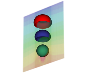
The major assumption in model H is the constant density of the mixture as well as of the individual constituents (making it not applicable to problems with large density ratios). This limitation initiated the generalization of model H to NSCH models with non-matching densities. Noteworthy contributions include the models of Lowengrub & Truskinovsky (Reference Lowengrub and Truskinovsky1998), Boyer (Reference Boyer2002), Ding, Spelt & Shu (Reference Ding, Spelt and Shu2007), Abels, Garcke & Grün (Reference Abels, Garcke and Grün2012), Shen, Yang & Wang (Reference Shen, Yang and Wang2013), Aki et al. (Reference Aki, Dreyer, Giesselmann and Kraus2014) and Shokrpour Roudbari et al. (Reference Shokrpour Roudbari, Şimşek, van Brummelen and van der Zee2018). The introduction of non-matching density models opened the door to practically relevant computations, such as the one in figure 1. Computations with NSCH models are non-trivial and require addressing issues such as bound preservation, interface accuracy and stability; for more details, see, e.g. Boyer et al. (Reference Boyer, Lapuerta, Minjeaud, Piar and Quintard2010), Minjeaud (Reference Minjeaud2013), Chen & Shen (Reference Chen and Shen2016), Khanwale et al. (Reference Khanwale, Saurabh, Ishii, Sundar, Rossmanith and Ganapathysubramanian2023). The above models all aim to describe the same physical phenomena (the evolution of isothermal incompressible mixtures), yet they are (seemingly) distinct from one another.

Figure 1. A representative bubble rising problem with large deformations with respect to the original bubble shape, computed with the NSCH model; see ten Eikelder & Schillinger (Reference ten Eikelder and Schillinger2024) for details.
In ten Eikelder et al. (Reference ten Eikelder, van der Zee, Akkerman and Schillinger2023) we have proposed a unified framework of existing Navier–Stokes Cahn–Hilliard Allen–Cahn (NSCHAC) models with non-matching densities. (This paper proposes a unified framework for NSCH models with non-zero mass fluxes. These mass fluxes follow the Allen–Cahn form, consequently, the framework can be referred to as a unified framework for NSCHAC models.) This framework leads to a single consistent NSCHAC system of balance laws, and shows that many alternate forms of the same model are connected via variable transformations. The term consistent conveys that this model is established in a consistent manner through continuum mixture theory. A particular formulation of the consistent NSCHAC model reads:
 \begin{gather} \partial_t (\rho \boldsymbol{v}) + {\rm div} ( \rho \boldsymbol{v}\otimes \boldsymbol{v} ) + \boldsymbol{\nabla} p + {\rm div} \left( \boldsymbol{\nabla} \phi \otimes \dfrac{\partial \bar{\varPsi}}{\partial \boldsymbol{\nabla} \phi} + (\bar{\mu}\phi-\bar{\varPsi})\boldsymbol{I} \right) \nonumber\\ -\, {\rm div} ( \nu (2\boldsymbol{D}+\lambda({\rm div}\,\boldsymbol{v}) \boldsymbol{I}) )-\rho\boldsymbol{b} = 0, \end{gather}
 $$\begin{gather} \partial_t \rho + {\rm div}(\rho \boldsymbol{v}) = 0, \end{gather}$$
 $$\begin{gather}\partial_t \phi + {\rm div}(\phi \boldsymbol{v}) - {\rm div} (\bar{\boldsymbol{M}}\boldsymbol{\nabla} (\bar{\mu}+\omega p)) +\zeta \bar{m} (\bar{\mu} + \omega p) =0, \end{gather}$$
 $$\begin{gather}\bar{\mu} - \dfrac{\partial \bar{\varPsi}}{\partial \phi}+{\rm div} \left( \dfrac{\partial \bar{\varPsi}}{\partial \boldsymbol{\nabla} \phi} \right)=0. \end{gather}$$
Here  $\rho$ is the mass-averaged mixture density, $\boldsymbol {v}$ the mixture velocity, $p$ the pressure, $\phi$ an order parameter and $\bar {\mu }$ a chemical potential quantity. Furthermore, $\bar {\boldsymbol {M}}=\bar {\boldsymbol {M}}(\phi,\boldsymbol {\nabla } \phi, \bar {\mu }, \boldsymbol {\nabla } \bar {\mu }, p)$ and $\bar {m}=\bar {m}(\phi, \bar {\mu }, p)$ are degenerate mobilities, $\nu$ the dynamic viscosity of the mixture, $\boldsymbol {g}$ the gravitational acceleration, $\rho _1$ and $\rho _2$ constant specific densities of the constituents, $\omega = (\rho _2-\rho _1)/(\rho _1+\rho _2)$ and $\zeta = (\rho _1+\rho _2)/(2\rho _1\rho _2)$. We provide precise definitions in § 5 and refer the reader to ten Eikelder et al. (Reference ten Eikelder, van der Zee, Akkerman and Schillinger2023) for details.
1.2. Objective and main results
The unified framework presented in ten Eikelder et al. (Reference ten Eikelder, van der Zee, Akkerman and Schillinger2023) completes the fundamental exploration of alternate non-matching density NSCHAC models. However, the NSCHAC model is not compatible with mixture theory of rational mechanics. Namely, in the construction of the NSCHAC model, the evolution equation of the diffusive flux that results from mixture theory is replaced by a constitutive model. Therefore, the NSCHAC model may be classified as a reduced mixture model. (The NSCHAC model may be classified as a class-I model; see Bothe (Reference Bothe2022) for details on this terminology.) This observation bring us to the main objective of this paper: to derive a thermodynamically consistent diffuse-interface incompressible mixture model compatible with continuum mixture theory. We restrict to isothermal constituents. The thermodynamically consistent property of the mixture model refers to the compatibility with the second law of thermodynamics. In particular, we derive the mixture model
 \begin{gather} \partial_t \tilde{\rho}_{\alpha} + {\rm div}(\tilde{\rho}_{\alpha} \boldsymbol{v}_{\alpha}) + \sum_{{\beta}} m_{\alpha{\beta}}(g_{\alpha}-g_{{\beta}}) = 0, \end{gather}
 \begin{gather} \partial_t
(\tilde{\rho}_{\alpha} \boldsymbol{v}_{\alpha}) + {\rm div}
( \tilde{\rho}_{\alpha} \boldsymbol{v}_{\alpha}\otimes
\boldsymbol{v}_{\alpha} ) +
\phi_{\alpha}\boldsymbol{\nabla} (\,p + \mu_{\alpha} )\nonumber\\
-\, {\rm div}(\tilde{\nu}_{\alpha}
(2\boldsymbol{D}_{\alpha} + \lambda_{\alpha} \,{\rm
div}\,\boldsymbol{v}_{\alpha}))
-\tilde{\rho}_{\alpha}\boldsymbol{b}\nonumber\\
+\,\sum_{{\beta}} R_{\alpha{\beta}}
(\boldsymbol{v}_{\alpha}-\boldsymbol{v}_{{\beta}}) +
\frac{1}{2}\sum_{{\beta}}
m_{\alpha{\beta}}(g_{\alpha}-g_{{\beta}})(\boldsymbol{v}_{\alpha}+\boldsymbol{v}_{{\beta}})
=0,
\end{gather}
\begin{gather} \partial_t
(\tilde{\rho}_{\alpha} \boldsymbol{v}_{\alpha}) + {\rm div}
( \tilde{\rho}_{\alpha} \boldsymbol{v}_{\alpha}\otimes
\boldsymbol{v}_{\alpha} ) +
\phi_{\alpha}\boldsymbol{\nabla} (\,p + \mu_{\alpha} )\nonumber\\
-\, {\rm div}(\tilde{\nu}_{\alpha}
(2\boldsymbol{D}_{\alpha} + \lambda_{\alpha} \,{\rm
div}\,\boldsymbol{v}_{\alpha}))
-\tilde{\rho}_{\alpha}\boldsymbol{b}\nonumber\\
+\,\sum_{{\beta}} R_{\alpha{\beta}}
(\boldsymbol{v}_{\alpha}-\boldsymbol{v}_{{\beta}}) +
\frac{1}{2}\sum_{{\beta}}
m_{\alpha{\beta}}(g_{\alpha}-g_{{\beta}})(\boldsymbol{v}_{\alpha}+\boldsymbol{v}_{{\beta}})
=0,
\end{gather}
for constituents  $\alpha = 1,\ldots,N$. Here $\tilde {\rho }_{\alpha }$ is the partial mass density of constituent $\alpha$, $\boldsymbol {v}_{\alpha }$ the constituent velocity, $\phi _{\alpha }$ the constituent volume fraction and $\mu _{\alpha }$ a constituent chemical potential. Furthermore, $p$ is the mechanical pressure, $\mu _{\alpha }$ the constituent chemical potential, $g_{\alpha }$ the constituent Gibbs free energy, $\tilde {\nu }_{\alpha }$ the constituent dynamical viscosity, $\lambda _{\alpha } \tilde {\nu }_{\alpha }$ the constituent second viscosity coefficient, $\boldsymbol {D}_{\alpha }$ the constituent symmetric velocity gradient, and $m_{\alpha {\beta }}$ and $R_{\alpha {\beta }}$ are symmetric matrices. We provide precise definitions in §§ 3 and 4.
The distinguishing feature of the model lies in the occurrence of both a mass and a momentum balance equation per constituent. Reduced models of NSCHAC type contain a phase equation per constituent but a single momentum equation for the mixture. This decrease in complexity comes at the cost of violating mixture theory of rational mechanics. Another interesting aspect is that the model has no Cahn–Hilliard-type equation; however, the equilibrium profile coincides with that of the NSCHAC model (for the standard Ginzburg–Landau free energy). On the other hand, the mass transfer terms match that of the Allen–Cahn equation, i.e. the model is of Allen–Cahn type. Another important feature of the model contains a single mixture mechanical pressure  $p$ (the Lagrange multiplier of the mixture incompressibility constraint) and a constituent chemical potential $\mu _{\alpha }$.
1.3. Plan of the paper
The remainder of the paper is structured as follows. In § 2 we present the general continuum theory of incompressible fluid mixtures. Here we present identities that relate constituent and mixture quantities. We exclude thermal effects. Next, in § 3 we perform constitutive modelling via the Coleman–Noll procedure. Then, in § 4 we present particular diffuse-interface models. We compare the resulting models with the NSCHAC model in § 5. Finally, in § 6 we conclude and outline avenues for future research.
2. Continuum theory of mixtures
The purpose of this section is to lay down the continuum theory of mixtures composed of incompressible isothermal constituents. The theory is based on three general principles proposed in the groundbreaking work of Truesdell & Toupin (Reference Truesdell and Toupin1960).
(i) All properties of the mixture must be mathematical consequences of properties of the constituents.
(ii) So as to describe the motion of a constituent, we may in imagination isolate it from the rest of the mixture, provided we allow properly for the actions of the other constituents upon it.
(iii) The motion of the mixture is governed by the same equations as is a single body.
The first principle states that the mixture is composed of its constituent parts. The second principle asserts the physics model be banded together via interaction fluxes, forces or energies. Finally, the third principle ensures that the motion of a mixture is indistinguishable from that of a single fluid.
In § 2.1 we introduce the fundamentals of the continuum theory of mixtures and the necessary kinematics. Then, in § 2.2 we provide balance laws of individual constituents and associated mixtures.
2.1. Preliminaries and kinematics
The core idea of the continuum theory of mixtures is that the material body  $\mathscr {B}$ is composed of $N$ constituent bodies $\mathscr {B}_{\alpha }$, with $\alpha = 1, \ldots, N$. Following Truesdell (Reference Truesdell1984), the bodies $\mathscr {B}_{\alpha }$ are allowed to occupy, simultaneously, a common region in space. Denote with $\boldsymbol {X}_{\alpha }$ the spatial position of a particle of $\mathscr {B}_{\alpha }$ in the Lagrangian (reference) configuration. The motion of body $\mathscr {B}_{\alpha }$ is given by the (invertible) deformation map
 \begin{equation} \boldsymbol{x} := \boldsymbol{\chi}_{\alpha}(\boldsymbol{X}_{\alpha},t). \end{equation}
Consider from now on positions  $\boldsymbol {x}$ that are taken by one particle from each of the $N$ constituent bodies $\mathscr {B}_{\alpha }$. Around this spatial position $\boldsymbol {x}$ we consider an arbitrary mixture control volume $V \subset \varOmega$ with measure $\vert V \vert$. Furthermore, we introduce volume $V_{\alpha } \subset V$, with measure $\vert V_{\alpha }\vert$, as the control volume of constituent $\alpha$. The constituents masses denote $M_{\alpha }=M_{\alpha }(V)$ and the total mass in $V$ is $M=M(V)=\sum _{\alpha }M_{\alpha }(V)$. The constituent partial mass density $\tilde {\rho }_{\alpha }$ and specific mass density $\rho _{\alpha }>0$ are respectively defined as
 $$\begin{gather} \tilde{\rho}_{\alpha}(\boldsymbol{x},t) :=\lim_{ \vert V \vert \rightarrow 0} \dfrac{M_{\alpha}(V)}{\vert V \vert}, \end{gather}$$
 $$\begin{gather}\rho_{\alpha}(\boldsymbol{x},t) := \lim_{\vert V_{\alpha}\vert \rightarrow 0} \dfrac{M_{\alpha}(V)}{\vert V_{\alpha}\vert }. \end{gather}$$
The quantities represent the mass of the associated constituent  $\alpha$ per unit volume of the mixture $V$, and constituent volume $V_{\alpha }$, respectively. In this paper we work with incompressible isothermal constituents of which the specific mass densities $\rho _{\alpha }$ are constants. The density of the mixture is the sum of the partial mass densities of the constituents:
 \begin{equation} \rho(\boldsymbol{x},t):=\sum_{\alpha}\tilde{\rho}_{\alpha}(\boldsymbol{x},t). \end{equation}
The volume fraction of constituent  $\alpha$ is defined as
 \begin{equation} \phi_{\alpha}(\boldsymbol{x},t) := \lim_{\vert V \vert \rightarrow 0} \dfrac{\vert V_{\alpha}\vert }{\vert V \vert}. \end{equation}
We preclude the existence of void spaces by assuming that
 \begin{equation} \sum_{\alpha} \phi_{\alpha}= 1. \end{equation}
The above definitions (2.2), (2.3) and (2.4) imply the relation
 \begin{equation} \tilde{\rho}_{\alpha}(\boldsymbol{x},t) = \rho_{\alpha}\phi_{\alpha}(\boldsymbol{x},t). \end{equation}
The constituent velocity is given by
 \begin{equation} \boldsymbol{v}_{\alpha}(\boldsymbol{x},t)=\partial_t\boldsymbol{\chi}_{\alpha}(\boldsymbol{X}_{\alpha},t) \vert_{\boldsymbol{X}_{\alpha}}, \end{equation}
where the position  $\boldsymbol {X}_{\alpha }$ is fixed. Next, we denote the momentum of constituent $\alpha$ as
 \begin{equation} \boldsymbol{m}_{\alpha}(\boldsymbol{x},t) = \tilde{\rho}_{\alpha}(\boldsymbol{x},t) \boldsymbol{v}_{\alpha}(\boldsymbol{x},t). \end{equation}
By taking the sum of the momenta of the constituent we get the momentum of the mixture:
 \begin{equation} \boldsymbol{m}(\boldsymbol{x},t) := \sum_{\alpha} \boldsymbol{m}_{\alpha}(\boldsymbol{x},t). \end{equation}
From the momentum of the mixture, we identify the mixture velocity  $\boldsymbol {v}$ (also called mass-averaged velocity or barycentric velocity):
 \begin{equation} \boldsymbol{m}(\boldsymbol{x},t) = \rho(\boldsymbol{x},t) \boldsymbol{v}(\boldsymbol{x},t). \end{equation}
Another important velocity is the peculiar velocity (also known as diffusion velocity) of constituent  $\alpha$, i.e.
 \begin{equation} \boldsymbol{w}_{\alpha}(\boldsymbol{x},t):=\boldsymbol{v}_{\alpha}(\boldsymbol{x},t)-\boldsymbol{v}(\boldsymbol{x},t), \end{equation}
which describes the constituent velocity relative to the gross motion of the mixture. The peculiar velocity satisfies the property
 \begin{equation} \sum_{\alpha} \boldsymbol{J}_{\alpha} = \sum_{\alpha} \rho_{\alpha} \boldsymbol{h}_{\alpha} = 0, \end{equation}
where the so-called diffusive fluxes are defined as
 $$\begin{gather} \boldsymbol{h}_{\alpha} := \phi_{\alpha}\boldsymbol{w}_{\alpha} , \end{gather}$$
 $$\begin{gather}\boldsymbol{J}_{\alpha} := \tilde{\rho}_{\alpha} \boldsymbol{w}_{\alpha}. \end{gather}$$
 We introduce the time derivative  $\grave {\psi }_{\alpha }$ of the (component) differentiable function $\psi _{\alpha }$ of $\boldsymbol {x}$ and $t$, and the time derivative of a quantity $\psi$ that follows the mean motion. In the Eulerian frame, these material derivatives are given by
 $$\begin{gather} \grave{\psi}_{\alpha}= \partial_t \psi_{\alpha} + \boldsymbol{v}_{\alpha}\boldsymbol{\cdot} \boldsymbol{\nabla} \psi_{\alpha}, \end{gather}$$
 $$\begin{gather}\dot{\psi} = \partial_t \psi + \boldsymbol{v}\boldsymbol{\cdot} \boldsymbol{\nabla} \psi. \end{gather}$$
2.2. Balance laws
According to the second general principle of the continuum theory of mixtures, the motion of each of the constituents is governed by an individual set of balance laws. These laws contain interaction terms that model the interplay of the different constituents. Following, e.g. Truesdell (Reference Truesdell1984), each of the constituent  $\alpha = 1, \ldots, N$ must satisfy the following set of local balance laws for all $\boldsymbol {x} \in \varOmega$ and $t \in (0,T)$:
 $$\begin{gather} \partial_t \tilde{\rho}_{\alpha} + {\rm div}(\tilde{\rho}_{\alpha} \boldsymbol{v}_{\alpha}) = \gamma_{\alpha}, \end{gather}$$
 $$\begin{gather}\partial_t \boldsymbol{m}_{\alpha} + {\rm div} ( \boldsymbol{m}_{\alpha}\otimes \boldsymbol{v}_{\alpha} ) - {\rm div} \,\boldsymbol{T}_{\alpha} - \tilde{\rho}_{\alpha} \boldsymbol{b}_{\alpha} = \boldsymbol{\rm \pi}_{\alpha}, \end{gather}$$
 $$\begin{gather}\boldsymbol{T}_{\alpha}-\boldsymbol{T}_{\alpha}^T =\boldsymbol{N}_{\alpha}, \end{gather}$$
 \begin{gather}
\partial_t (\tilde{\rho}_{\alpha}
(\epsilon_{\alpha}+\|\boldsymbol{v}_{\alpha}\|^2/2)) + {\rm
div} ( \tilde{\rho}_{\alpha}(\epsilon_{\alpha} +
\|\boldsymbol{v}_{\alpha}\|^2/2)\boldsymbol{v}_{\alpha} ) \nonumber\\
-\,{\rm div}(\boldsymbol{T}_{\alpha} \boldsymbol{v}_{\alpha} ) - \tilde{\rho}_{\alpha}
\boldsymbol{b}_{\alpha}\boldsymbol{\cdot}\boldsymbol{v}_{\alpha}
+ {\rm div} \,\boldsymbol{q}_{\alpha} -
\tilde{\rho}_{\alpha} r_{\alpha} =e_{\alpha}.
\end{gather}
\begin{gather}
\partial_t (\tilde{\rho}_{\alpha}
(\epsilon_{\alpha}+\|\boldsymbol{v}_{\alpha}\|^2/2)) + {\rm
div} ( \tilde{\rho}_{\alpha}(\epsilon_{\alpha} +
\|\boldsymbol{v}_{\alpha}\|^2/2)\boldsymbol{v}_{\alpha} ) \nonumber\\
-\,{\rm div}(\boldsymbol{T}_{\alpha} \boldsymbol{v}_{\alpha} ) - \tilde{\rho}_{\alpha}
\boldsymbol{b}_{\alpha}\boldsymbol{\cdot}\boldsymbol{v}_{\alpha}
+ {\rm div} \,\boldsymbol{q}_{\alpha} -
\tilde{\rho}_{\alpha} r_{\alpha} =e_{\alpha}.
\end{gather}
Equation (2.15a) represents the local constituent mass balance law, where the interaction term  $\gamma _{\alpha }$ is the mass supply of constituent $\alpha$ due to chemical reactions with the other constituents. Next, (2.15b) is the local constituent linear momentum balance law. Here $\boldsymbol {T}_{\alpha }$ is the Cauchy stress tensor of constituent $\alpha$, $\boldsymbol {b}_{\alpha }$ the constituent external body force and ${\boldsymbol {{\rm \pi} }}_{\alpha }$ is the momentum exchange rate of constituent $\alpha$ with the other constituents. In the remainder of the paper we assume equal body forces ( $\boldsymbol {b}_{\alpha }= \boldsymbol {b}$ for $\alpha = 1, \ldots, N$). Moreover, we restrict to body forces of a gravitational type: $\boldsymbol {b} = -b \boldsymbol {\jmath } = -b \boldsymbol {\nabla } y$, with $y$ the vertical coordinate, $\boldsymbol {\jmath }$ the vertical unit vector and $b$ a constant. Next, (2.15c) is the local constituent angular momentum balance with $\boldsymbol {N}_{\alpha }$ the intrinsic moment of momentum. Finally, (2.15d) is the local constituent energy balance. Here $\epsilon _{\alpha }$ is the specific internal energy of constituent $\alpha$, $\|\boldsymbol {v}_{\alpha }\|=\sqrt {\boldsymbol {v}_{\alpha } \boldsymbol{\cdot} \boldsymbol {v}_{\alpha }}$ is the Euclidean norm of the velocity $\boldsymbol {v}_{\alpha }$, $\boldsymbol {q}_{\alpha }$ is the heat flux, $r_{\alpha }$ is the external heat supply and $e_{\alpha }$ represents the energy exchange with the other constituents.
We denote the kinetic and gravitational energies of the constituents, respectively, as
 $$\begin{gather} \mathscr{K}_{\alpha} =\tilde{\rho}_{\alpha} \|\boldsymbol{v}_{\alpha}\|^2/2, \end{gather}$$
 $$\begin{gather}\mathscr{G}_{\alpha} =\tilde{\rho}_{\alpha} b y. \end{gather}$$
On the account of the mass balance (2.15a) and the linear momentum balance (2.15b), we deduce the evolution of the constituent kinetic energy:
 \begin{equation} \partial_t \mathscr{K}_{\alpha} + {\rm div}( \mathscr{K}_{\alpha} \boldsymbol{v}_{\alpha} ) - \boldsymbol{v}_{\alpha}\boldsymbol{\cdot} {\rm div} \,\boldsymbol{T}_{\alpha} - \tilde{\rho}_{\alpha} \boldsymbol{b}_{\alpha} \boldsymbol{\cdot} \boldsymbol{v}_{\alpha}= \boldsymbol{\rm \pi}_{\alpha}\boldsymbol{\cdot}\boldsymbol{v}_{\alpha} - \tfrac{1}{2}\|\boldsymbol{v}_{\alpha}\|^2 \gamma_{\alpha}. \end{equation}
Next, the evolution of the gravitational energy follows from the constituent mass equation (2.15a):
 \begin{equation} \partial_t \mathscr{G}_{\alpha} + {\rm div}( \mathscr{G}_{\alpha} \boldsymbol{v}_{\alpha} ) + \tilde{\rho}_{\alpha} \boldsymbol{v}_{\alpha}\boldsymbol{\cdot} \boldsymbol{b} - \gamma_{\alpha} b y=0. \end{equation}
Taking the difference of (2.15d) and (2.17) we obtain the evolution of the constituent internal energy:
 \begin{gather} \partial_t
(\tilde{\rho}_{\alpha} \epsilon_{\alpha}) + {\rm div} (
\tilde{\rho}_{\alpha}\epsilon_{\alpha}
\boldsymbol{v}_{\alpha} ) - \boldsymbol{T}_{\alpha}:
\boldsymbol{\nabla} \boldsymbol{v}_{\alpha} + {\rm div}
\,\boldsymbol{q}_{\alpha} - \tilde{\rho}_{\alpha}
r_{\alpha} \nonumber\\ \quad =-
\boldsymbol{\rm \pi}_{\alpha}\boldsymbol{\cdot}\boldsymbol{v}_{\alpha}
+ \tfrac{1}{2}\|\boldsymbol{v}_{\alpha}\|^2 \gamma_{\alpha}
+ e_{\alpha} .
\end{gather}
\begin{gather} \partial_t
(\tilde{\rho}_{\alpha} \epsilon_{\alpha}) + {\rm div} (
\tilde{\rho}_{\alpha}\epsilon_{\alpha}
\boldsymbol{v}_{\alpha} ) - \boldsymbol{T}_{\alpha}:
\boldsymbol{\nabla} \boldsymbol{v}_{\alpha} + {\rm div}
\,\boldsymbol{q}_{\alpha} - \tilde{\rho}_{\alpha}
r_{\alpha} \nonumber\\ \quad =-
\boldsymbol{\rm \pi}_{\alpha}\boldsymbol{\cdot}\boldsymbol{v}_{\alpha}
+ \tfrac{1}{2}\|\boldsymbol{v}_{\alpha}\|^2 \gamma_{\alpha}
+ e_{\alpha} .
\end{gather}The convective forms of the constituent evolution equations read
 $$\begin{gather} \grave{\tilde{\rho}}_{\alpha} +\tilde{\rho}_{\alpha} \,{\rm div}\,\boldsymbol{v}_{\alpha} =\gamma_{\alpha}, \end{gather}$$
 $$\begin{gather}\tilde{\rho}_{\alpha} \grave{\boldsymbol{v}}_{\alpha} - {\rm div} \,\boldsymbol{T}_{\alpha} - \tilde{\rho}_{\alpha} \boldsymbol{b}_{\alpha}=\boldsymbol{p}_{\alpha}, \end{gather}$$
 $$\begin{gather}\tilde{\rho}_{\alpha} \grave{\epsilon}_{\alpha} -\boldsymbol{T}_{\alpha}: \boldsymbol{\nabla} \boldsymbol{v}_{\alpha} + {\rm div}\, \boldsymbol{q}_{\alpha} -\tilde{\rho}_{\alpha} r_{\alpha} =\breve{e}_{\alpha}, \end{gather}$$
where the interaction terms are
 $$\begin{gather} \boldsymbol{p}_{\alpha} = \boldsymbol{\rm \pi}_{\alpha} - \gamma_{\alpha} \boldsymbol{v}_{\alpha}, \end{gather}$$
 $$\begin{gather}\breve{e}_{\alpha} = e_{\alpha} - \boldsymbol{\rm \pi}_{\alpha} \boldsymbol{\cdot} \boldsymbol{v}_{\alpha} - \gamma_{\alpha} (\epsilon_{\alpha} - \|\boldsymbol{v}_{\alpha}\|^2/2). \end{gather}$$
By invoking the constant specific densities  $\rho _{\alpha }$, we obtain the evolution equation of the volume fraction:
 \begin{equation} \partial_t \phi_{\alpha} + {\rm div}(\phi_{\alpha} \boldsymbol{v}_{\alpha})= \dfrac{\gamma_{\alpha}}{\rho_{\alpha}}. \end{equation}
Next, we turn to the continuum balance laws of the mixtures. Summing the balance laws (2.15) over the constituents gives
 $$\begin{gather} \partial_t \rho + {\rm div}(\rho \boldsymbol{v}) = 0, \end{gather}$$
 $$\begin{gather}\partial_t \boldsymbol{m} + {\rm div} ( \boldsymbol{m}\otimes \boldsymbol{v} ) - {\rm div} \,\boldsymbol{T} - \rho \boldsymbol{b} =0, \end{gather}$$
 $$\begin{gather}\boldsymbol{T}-\boldsymbol{T}^T =0, \end{gather}$$
 \begin{gather}
\partial_t (\rho (\epsilon+\|\boldsymbol{v}\|^2/2)) + {\rm
div} ( \rho(\epsilon +
\|\boldsymbol{v}\|^2/2)\boldsymbol{v} )\nonumber\\
-\, {\rm div}( \boldsymbol{T}\boldsymbol{v})- \rho
\boldsymbol{b}\boldsymbol{\cdot}\boldsymbol{v} +{\rm
div}\,\boldsymbol{q}- \rho r =0,
\end{gather}
\begin{gather}
\partial_t (\rho (\epsilon+\|\boldsymbol{v}\|^2/2)) + {\rm
div} ( \rho(\epsilon +
\|\boldsymbol{v}\|^2/2)\boldsymbol{v} )\nonumber\\
-\, {\rm div}( \boldsymbol{T}\boldsymbol{v})- \rho
\boldsymbol{b}\boldsymbol{\cdot}\boldsymbol{v} +{\rm
div}\,\boldsymbol{q}- \rho r =0,
\end{gather}where
 $$\begin{gather} \epsilon := \frac{1}{\rho}\sum_{\alpha} \tilde{\rho}_{\alpha} \bigg(\epsilon_{\alpha} + \frac{1}{2} \|\boldsymbol{w}_{\alpha} \|^2 \bigg), \end{gather}$$
 $$\begin{gather}\boldsymbol{T} := \sum_{\alpha} \boldsymbol{T}_{\alpha}-\tilde{\rho}_{\alpha}\boldsymbol{w}_{\alpha}\otimes\boldsymbol{w}_{\alpha}, \end{gather}$$
 $$\begin{gather}\boldsymbol{b} :=\frac{1}{\rho}\sum_{\alpha} \tilde{\rho}_{\alpha}\boldsymbol{b}_{\alpha}, \end{gather}$$
 $$\begin{gather}\boldsymbol{q} := \sum_{\alpha} \boldsymbol{q}_{\alpha} - \boldsymbol{T}_{\alpha} \boldsymbol{w}_{\alpha} + \tilde{\rho}_{\alpha} \bigg(\epsilon_{\alpha} + \frac{1}{2}\|\boldsymbol{w}_{\alpha} \|^2\bigg), \end{gather}$$
 $$\begin{gather}r:=\frac{1}{\rho}\sum_{\alpha} \tilde{\rho}_{\alpha} r_{\alpha}, \end{gather}$$
and where we have postulated the following balance conditions to hold:
 $$\begin{gather} \sum_{\alpha} \gamma_{\alpha} = 0, \end{gather}$$
 $$\begin{gather}\sum_{\alpha} \boldsymbol{\rm \pi}_{\alpha} = 0, \end{gather}$$
 $$\begin{gather}\sum_{\alpha} \boldsymbol{N}_{\alpha} = 0, \end{gather}$$
 $$\begin{gather}\sum_{\alpha} e_{\alpha} = 0. \end{gather}$$
In establishing the mixture laws (2.23) use has been made of the identities (2.12) and
 \begin{equation} \sum_{\alpha} \tilde{\rho}_{\alpha} \frac{1}{2}\|\boldsymbol{w}_{\alpha} \|^2\boldsymbol{w}_{\alpha} = \sum_{\alpha} \bigg(\tilde{\rho}_{\alpha} \frac{1}{2}\|\boldsymbol{v}_{\alpha} \|^2\boldsymbol{w}_{\alpha} - \tilde{\rho}_{\alpha} \boldsymbol{w}_{\alpha} (\boldsymbol{w}_{\alpha}\boldsymbol{\cdot} \boldsymbol{v})\bigg). \end{equation}
In agreement with the first general principle of mixture theory, the kinetic, gravitational and internal energies of the mixture are the superposition of the constituent energies:
 $$\begin{gather} \mathscr{K} =\sum_{\alpha} \mathscr{K}_{\alpha}, \end{gather}$$
 $$\begin{gather}\mathscr{G} =\sum_{\alpha} \mathscr{G}_{\alpha}, \end{gather}$$
 $$\begin{gather}\mathscr{S} = \sum_{\alpha} \tilde{\rho}_{\alpha} \epsilon_{\alpha}. \end{gather}$$
The kinetic energy of the mixture can be decomposed as
 $$\begin{gather} \mathscr{K} = \bar{\mathscr{K}} + \displaystyle\sum_{\alpha} \frac{1}{2} \tilde{\rho}_{\alpha} \|\boldsymbol{w}_{\alpha}\|^2, \end{gather}$$
 $$\begin{gather}\bar{\mathscr{K}} = \frac{1}{2} \rho \|\boldsymbol{v}\|^2, \end{gather}$$
where  $\bar {\mathscr {K}}$ is a kinetic energy of the mixture variables, and where the second term represents the kinetic energy of the constituents relative to the gross motion of the mixture. As a consequence, (2.15d) represents the evolution of the internal and kinetic energy of the mixture
 \begin{equation} \partial_t \mathscr{E} + {\rm div} ( \mathscr{E}\boldsymbol{v} ) -{\rm div}( \boldsymbol{T}\boldsymbol{v} )- \rho \boldsymbol{b}\boldsymbol{\cdot}\boldsymbol{v} +{\rm div}\,\boldsymbol{q}- \rho r=0, \end{equation}
with  $\mathscr {E} = \mathscr {K}+\mathscr {G}+\mathscr {S}$, given the standing assumption of equal body forces. Finally, we remark that the system of mixture balance laws (2.23) may be augmented with evolution equations of the order parameters (mass and energy) and diffusive fluxes to arrive at a system equivalent with (2.15) (ten Eikelder et al. Reference ten Eikelder, van der Zee, Akkerman and Schillinger2023).
3. Constitutive modelling
In this section we perform the constitutive modelling. We choose to employ the well-known Coleman–Noll procedure (Coleman & Noll Reference Coleman and Noll1974) to construct constitutive models that satisfy the second law of thermodynamics. First, in § 3.1 we introduce the second law of thermodynamics in the context of rational mechanics. Next, in § 3.2 we establish the constitutive modelling restriction yielding from the second law. Then, in § 3.3 we select specific constitutive models compatible with the modelling restriction.
3.1. Second law
In agreement with the second general principle, the entropy of each of the constituents  $\alpha$ is governed by the balance law
 \begin{equation} \partial_t (\tilde{\rho}_{\alpha} \eta_{\alpha}) + {\rm div}( \tilde{\rho}_{\alpha} \eta_{\alpha} \boldsymbol{v}_{\alpha} ) + {\rm div} (\boldsymbol{\varPhi}_{\alpha}) - \tilde{\rho}_{\alpha} s_{\alpha} =\mathscr{P}_{\alpha}, \end{equation}
where the constituent quantities are the specific entropy density  $\eta _{\alpha }$, the entropy flux $\boldsymbol {\varPhi }_{\alpha }$, the specific entropy supply $s_{\alpha }$ and the entropy production $\mathscr {P}_{\alpha }$. The second law of thermodynamics dictates positive entropy production of the entire mixture:
 \begin{equation} \sum_{\alpha} \mathscr{P}_{\alpha} \geq 0. \end{equation}
The second law (3.2) is compatible with the first general principle of mixture theory.
In the following we derive the modelling restriction that results from the second law (3.2). To this purpose, we introduce the Helmholtz mass-measure free energy of constituent  $\alpha$,
 \begin{equation} \psi_{\alpha} := \epsilon_{\alpha} - \theta \eta_{\alpha}, \end{equation}
where  $\theta$ is the temperature. We restrict to isothermal mixtures and, thus, all constituents have the same constant temperature $\theta = \theta _{\alpha }$, $\alpha = 1, \ldots, N$. We now substitute (3.1) and (3.3) into (3.2) and arrive at
 \begin{equation} \sum_{\alpha} \partial_t (\tilde{\rho}_{\alpha} (\epsilon_{\alpha}-\psi_{\alpha})) + {\rm div}( \tilde{\rho}_{\alpha} (\epsilon_{\alpha}-\psi_{\alpha}) \boldsymbol{v}_{\alpha} ) + {\rm div} (\theta\boldsymbol{\varPhi}_{\alpha}) - \tilde{\rho}_{\alpha} s_{\alpha} \theta \geq 0. \end{equation}
Next, we insert the balance of energy (2.19) into (3.4) and find that
 \begin{align} &\sum_{\alpha} -\partial_t (\tilde{\rho}_{\alpha} \psi_{\alpha}) - {\rm div} ( \tilde{\rho}_{\alpha} \psi_{\alpha} \boldsymbol{v}_{\alpha} ) +\boldsymbol{T}_{\alpha}: \boldsymbol{\nabla} \boldsymbol{v}_{\alpha}+ {\rm div} (\theta \boldsymbol{\varPhi}_{\alpha}-\boldsymbol{q}_{\alpha}) \nonumber\\ &\quad + \tilde{\rho}_{\alpha} (r_{\alpha} -\theta s_{\alpha}) -\boldsymbol{\rm \pi}_{\alpha}\boldsymbol{\cdot}\boldsymbol{v}_{\alpha}+ \gamma_{\alpha} \|\boldsymbol{v}_{\alpha}\|^2/2\geq 0, \end{align}
where the energy interaction term cancels because of (2.25d). In the final step we invoke the mass balance equation (2.15a) to find that
 \begin{align} &\sum_{\alpha} \tilde{\rho}_{\alpha}\grave{\psi}_{\alpha} - \boldsymbol{T}_{\alpha}:\boldsymbol{\nabla} \boldsymbol{v}_{\alpha} + {\rm div}(\boldsymbol{q}_{\alpha}-\theta\boldsymbol{\varPhi}_{\alpha})\nonumber\\ &\quad +\tilde{\rho}_{\alpha} (\theta s_{\alpha}-r_{\alpha}) +\boldsymbol{\rm \pi}_{\alpha}\boldsymbol{\cdot}\boldsymbol{v}_{\alpha}- \gamma_{\alpha} \|\boldsymbol{v}_{\alpha}\|^2/2 + \gamma_{\alpha} \psi_{\alpha} \leq 0. \end{align}
This form of the second law provides the basis for the constitutive modelling.
Lastly, we remark that the second law may be written in an energy-dissipative form (given  $r_{\alpha } = \theta s_{\alpha }$).
Proposition 3.1 (Energy dissipation)
The second law may be written as the energy-dissipation statement:
 \begin{equation} \sum_{\alpha}(\partial_t \mathscr{E}_{\alpha} + {\rm div}(\mathscr{E}_{\alpha}\boldsymbol{v}_{\alpha} ) - {\rm div} (\boldsymbol{T}_{\alpha}\boldsymbol{v}_{\alpha} - \boldsymbol{q}_{\alpha}+\theta\boldsymbol{\varPhi}_{\alpha}))\leq 0, \end{equation}
with  $\mathscr {E}_{\alpha } = \mathscr {K}_{\alpha }+\mathscr {G}_{\alpha }+\tilde {\rho }_{\alpha } \epsilon _{\alpha }$, and where we have set $r_{\alpha } = \theta s_{\alpha }$.
Proof. Using the constituent mass equation (2.15a), the second law (3.6) may be written as
 \begin{align} &\sum_{\alpha} [\partial_t (\tilde{\rho}_{\alpha}\psi_{\alpha}) + {\rm div}(\tilde{\rho}_{\alpha} \psi_{\alpha} \boldsymbol{v}_{\alpha}) - \boldsymbol{T}_{\alpha}:\boldsymbol{\nabla} \boldsymbol{v}_{\alpha} + {\rm div}(\boldsymbol{q}_{\alpha}-\theta\boldsymbol{\varPhi}_{\alpha}) \nonumber\\ &\quad +\boldsymbol{\rm \pi}_{\alpha}\boldsymbol{\cdot}\boldsymbol{v}_{\alpha}-e_{\alpha}- \gamma_{\alpha} \|\boldsymbol{v}_{\alpha}\|^2/2 ] \leq 0. \end{align}
Adding (2.17) and (2.18) to the condition (3.8) provides the result.
3.2. Constitutive modelling restriction
We specify the modelling restriction (3.6) to a particular set of constitutive constituent classes for the stress  $\boldsymbol {T}_{\alpha }$, free energy $\psi _{\alpha }$, entropy flux $\boldsymbol {\varPhi }_{\alpha }$, momentum supply $\boldsymbol {{\rm \pi} }_{\alpha }$ and mass supply $\gamma _{\alpha }$. We introduce the constitutive free energy class
 \begin{equation} \hat{\psi}_{\alpha} = \hat{\psi}_{\alpha}(\phi_{\alpha},\boldsymbol{\nabla} \phi_{\alpha}, \boldsymbol{D}_{\alpha}), \end{equation}
and postpone the specification of the other constitutive classes. Here  $\boldsymbol {D}_{\alpha }$ is the symmetric velocity gradient of constituent $\alpha$.
In the following we examine the constitutive modelling restriction (3.6) for this specific set of constitutive classes. Substitution of the constitutive classes (3.9) into (3.6) and expanding the peculiar derivative of the free energy provides
 \begin{align} &\sum_{\alpha}
\tilde{\rho}_{\alpha}\Bigg(\dfrac{\partial
\hat{\psi}_{\alpha}}{\partial
\phi_{\alpha}}\grave{\phi}_{\alpha}+\dfrac{\partial
\hat{\psi}_{\alpha}}{\partial
\boldsymbol{\nabla}\phi_{\alpha}}\boldsymbol{\cdot}\grave{\overline{\boldsymbol{\nabla}\phi}}_{\alpha}
+\partial_{\boldsymbol{D}_{\alpha}}\hat{\psi}_{\alpha}\grave{\boldsymbol{D}}_{\alpha}\Bigg)
-
\hat{\boldsymbol{T}}_{\alpha}:\boldsymbol{\nabla}\boldsymbol{v}_{\alpha}
\nonumber\\ &\quad + {\rm div}
(\boldsymbol{q}_{\alpha}-\theta\hat{\boldsymbol{\varPhi}}_{\alpha})
+\tilde{\rho}_{\alpha} (\theta s_{\alpha}-r_{\alpha})
\nonumber\\ &\quad
+\boldsymbol{\rm \pi}_{\alpha}\boldsymbol{\cdot}\boldsymbol{v}_{\alpha}-
\gamma_{\alpha} \|\boldsymbol{v}_{\alpha}\|^2/2 +
\gamma_{\alpha} \psi_{\alpha} \leq 0.
\end{align}
\begin{align} &\sum_{\alpha}
\tilde{\rho}_{\alpha}\Bigg(\dfrac{\partial
\hat{\psi}_{\alpha}}{\partial
\phi_{\alpha}}\grave{\phi}_{\alpha}+\dfrac{\partial
\hat{\psi}_{\alpha}}{\partial
\boldsymbol{\nabla}\phi_{\alpha}}\boldsymbol{\cdot}\grave{\overline{\boldsymbol{\nabla}\phi}}_{\alpha}
+\partial_{\boldsymbol{D}_{\alpha}}\hat{\psi}_{\alpha}\grave{\boldsymbol{D}}_{\alpha}\Bigg)
-
\hat{\boldsymbol{T}}_{\alpha}:\boldsymbol{\nabla}\boldsymbol{v}_{\alpha}
\nonumber\\ &\quad + {\rm div}
(\boldsymbol{q}_{\alpha}-\theta\hat{\boldsymbol{\varPhi}}_{\alpha})
+\tilde{\rho}_{\alpha} (\theta s_{\alpha}-r_{\alpha})
\nonumber\\ &\quad
+\boldsymbol{\rm \pi}_{\alpha}\boldsymbol{\cdot}\boldsymbol{v}_{\alpha}-
\gamma_{\alpha} \|\boldsymbol{v}_{\alpha}\|^2/2 +
\gamma_{\alpha} \psi_{\alpha} \leq 0.
\end{align}
The arbitrariness of the peculiar time derivative  $\grave {\boldsymbol {D}}_{\alpha }$ precludes dependence of $\psi _{\alpha }$ on $\boldsymbol {D}_{\alpha }$. Thus, the free energy class reduces to
 \begin{equation} \hat{\psi}_{\alpha} =\hat{\psi}_{\alpha} (\phi_{\alpha},\boldsymbol{\nabla} \phi_{\alpha}), \end{equation}
and the last member in the first brackets of (3.10) is eliminated. We now introduce the volumetric Helmholtz free energy  $\hat {\varPsi }_{\alpha }:=\tilde {\rho }_{\alpha }\hat {\psi }_{\alpha }$. Given the constituent class of $\hat {\psi }_{\alpha }$ (3.11), we identify the volumetric Helmholtz free energy class:
 \begin{equation} \hat{\varPsi}_{\alpha}=\hat{\varPsi}_{\alpha}(\phi_{\alpha},\boldsymbol{\nabla} \phi_{\alpha})=\tilde{\rho}_{\alpha}\hat{\psi}_{\alpha}(\phi_{\alpha},\boldsymbol{\nabla}\phi_{\alpha}) =\rho_{\alpha}\phi_{\alpha}\hat{\psi}_{\alpha}(\phi_{\alpha},\boldsymbol{\nabla} \phi_{\alpha}). \end{equation}
Next we introduce a number of constituent generalized derivatives of the free energy quantities that we require in examining the constitutive modelling restriction (3.6):
 $$\begin{gather} \chi_{\alpha} = \phi_{\alpha} \dfrac{ \partial \hat{\psi}_{\alpha}}{\partial \phi_{\alpha}} - {\rm div}\Bigg(\phi_{\alpha}\dfrac{\partial \hat{\psi}_{\alpha}}{\partial \boldsymbol{\nabla}\phi_{\alpha}}\Bigg), \end{gather}$$
 $$\begin{gather}\upsilon_{\alpha} = \dfrac{ \partial \hat{\psi}_{\alpha}}{\partial \tilde{\rho}_{\alpha}} - \dfrac{1}{\tilde{\rho}_{\alpha}}{\rm div}\Bigg(\tilde{\rho}_{\alpha}\dfrac{\partial \hat{\psi}_{\alpha}}{\partial \boldsymbol{\nabla}\tilde{\rho}_{\alpha}}\Bigg), \end{gather}$$
 $$\begin{gather}\tau_{\alpha} = \dfrac{\partial \hat{\psi}_{\alpha}}{\partial\phi_{\alpha}} - {\rm div}\Bigg( \dfrac{\partial \hat{\psi}_{\alpha}}{\partial \boldsymbol{\nabla} \phi_{\alpha}} \Bigg), \end{gather}$$
 $$\begin{gather}\mu_{\alpha} = \dfrac{ \partial \hat{\varPsi}_{\alpha}}{\partial \phi_{\alpha}} - {\rm div}\Bigg(\dfrac{\partial \hat{\varPsi}_{\alpha}}{\partial \boldsymbol{\nabla}\phi_{\alpha}}\Bigg). \end{gather}$$
Here  $\tau _{\alpha }$ is a mass-measure-based chemical potential and $\mu _{\alpha }$ is a volume-measure-based chemical potential. These quantities are related via the following identities:
 $$\begin{gather} \chi_{\alpha} = \tilde{\rho}_{\alpha} \upsilon_{\alpha}, \end{gather}$$
 $$\begin{gather}\mu_{\alpha} = \rho_{\alpha} (\hat{\psi}_{\alpha} + \chi_{\alpha} ), \end{gather}$$
 $$\begin{gather}\tilde{\rho}_{\alpha}\chi_{\alpha} = \phi_{\alpha} \mu_{\alpha} - \hat{\varPsi}_{\alpha}, \end{gather}$$
 $$\begin{gather}\chi_{\alpha} = \phi_{\alpha} \tau_{\alpha} - \boldsymbol{\nabla} \phi_{\alpha} \boldsymbol{\cdot} \dfrac{\partial \hat{\varPsi}_{\alpha}}{\partial \boldsymbol{\nabla}\phi_{\alpha}}. \end{gather}$$
Next, we focus on the first term in the sum in (3.10).
Lemma 3.2 (Identity peculiar derivative free energy)
We have the identity
 \begin{align}
\tilde{\rho}_{\alpha}\Bigg(\dfrac{\partial
\hat{\psi}_{\alpha}}{\partial
\phi_{\alpha}}\grave{\phi}_{\alpha}+\dfrac{\partial
\hat{\psi}_{\alpha}}{\partial
\boldsymbol{\nabla}\phi_{\alpha}}\boldsymbol{\cdot}\grave{\overline{\boldsymbol{\nabla}\phi}}_{\alpha}\Bigg)
&=-\tilde{\rho}_{\alpha}\Bigg(\chi_{\alpha}\,{\rm
div}\,\boldsymbol{v}_{\alpha}+\Bigg(\boldsymbol{\nabla}
\phi_{\alpha} \otimes \dfrac{\partial
\hat{\psi}_{\alpha}}{\partial
\boldsymbol{\nabla}\phi_{\alpha}}\Bigg):
\boldsymbol{\nabla}\boldsymbol{v}_{\alpha}\Bigg)\nonumber\\
&\quad -{\rm div}\Bigg(\tilde{\rho}_{\alpha}\dfrac{\partial
\hat{\psi}_{\alpha}}{\partial
\boldsymbol{\nabla}\phi_{\alpha}}(\phi_{\alpha}\,{\rm div}
\,\boldsymbol{v}_{\alpha})\Bigg)\nonumber\\ &\quad
+\gamma_{\alpha} \chi_{\alpha} + {\rm
div}\Bigg(\gamma_{\alpha}\phi_{\alpha} \dfrac{\partial
\hat{\psi}_{\alpha}}{\partial \boldsymbol{\nabla}
\phi_{\alpha}}\Bigg).
\end{align}
\begin{align}
\tilde{\rho}_{\alpha}\Bigg(\dfrac{\partial
\hat{\psi}_{\alpha}}{\partial
\phi_{\alpha}}\grave{\phi}_{\alpha}+\dfrac{\partial
\hat{\psi}_{\alpha}}{\partial
\boldsymbol{\nabla}\phi_{\alpha}}\boldsymbol{\cdot}\grave{\overline{\boldsymbol{\nabla}\phi}}_{\alpha}\Bigg)
&=-\tilde{\rho}_{\alpha}\Bigg(\chi_{\alpha}\,{\rm
div}\,\boldsymbol{v}_{\alpha}+\Bigg(\boldsymbol{\nabla}
\phi_{\alpha} \otimes \dfrac{\partial
\hat{\psi}_{\alpha}}{\partial
\boldsymbol{\nabla}\phi_{\alpha}}\Bigg):
\boldsymbol{\nabla}\boldsymbol{v}_{\alpha}\Bigg)\nonumber\\
&\quad -{\rm div}\Bigg(\tilde{\rho}_{\alpha}\dfrac{\partial
\hat{\psi}_{\alpha}}{\partial
\boldsymbol{\nabla}\phi_{\alpha}}(\phi_{\alpha}\,{\rm div}
\,\boldsymbol{v}_{\alpha})\Bigg)\nonumber\\ &\quad
+\gamma_{\alpha} \chi_{\alpha} + {\rm
div}\Bigg(\gamma_{\alpha}\phi_{\alpha} \dfrac{\partial
\hat{\psi}_{\alpha}}{\partial \boldsymbol{\nabla}
\phi_{\alpha}}\Bigg).
\end{align}Proof. Noting the identity
 \begin{equation} \grave{\overline{\boldsymbol{\nabla} \phi_{\alpha}}} = \boldsymbol{\nabla} (\grave{\phi}_{\alpha}) -(\boldsymbol{\nabla} \phi_{\alpha})^T \boldsymbol{\nabla} \boldsymbol{v}_{\alpha}, \end{equation}
we can deduce that
 \begin{align}
\tilde{\rho}_{\alpha}\dfrac{\partial
\hat{\psi}_{\alpha}}{\partial
\boldsymbol{\nabla}\phi_{\alpha}}\boldsymbol{\cdot}\grave{\overline{\boldsymbol{\nabla}
\phi_{\alpha}}} &= {\rm
div}\Bigg(\tilde{\rho}_{\alpha}\dfrac{\partial
\hat{\psi}_{\alpha}}{\partial
\boldsymbol{\nabla}\phi_{\alpha}}\grave{\phi}_{\alpha}\Bigg)-\grave{\phi}_{\alpha}\,{\rm
div} \Bigg( \tilde{\rho}_{\alpha}\dfrac{\partial
\hat{\psi}_{\alpha}}{\partial
\boldsymbol{\nabla}\phi_{\alpha}}\Bigg)\nonumber\\ &\quad
-\tilde{\rho}_{\alpha}\boldsymbol{\nabla} \phi_{\alpha}
\otimes \dfrac{\partial \hat{\psi}_{\alpha}}{\partial
\boldsymbol{\nabla}\phi_{\alpha}}\boldsymbol{\cdot}
\boldsymbol{\nabla}\boldsymbol{v}_{\alpha}.
\end{align}
\begin{align}
\tilde{\rho}_{\alpha}\dfrac{\partial
\hat{\psi}_{\alpha}}{\partial
\boldsymbol{\nabla}\phi_{\alpha}}\boldsymbol{\cdot}\grave{\overline{\boldsymbol{\nabla}
\phi_{\alpha}}} &= {\rm
div}\Bigg(\tilde{\rho}_{\alpha}\dfrac{\partial
\hat{\psi}_{\alpha}}{\partial
\boldsymbol{\nabla}\phi_{\alpha}}\grave{\phi}_{\alpha}\Bigg)-\grave{\phi}_{\alpha}\,{\rm
div} \Bigg( \tilde{\rho}_{\alpha}\dfrac{\partial
\hat{\psi}_{\alpha}}{\partial
\boldsymbol{\nabla}\phi_{\alpha}}\Bigg)\nonumber\\ &\quad
-\tilde{\rho}_{\alpha}\boldsymbol{\nabla} \phi_{\alpha}
\otimes \dfrac{\partial \hat{\psi}_{\alpha}}{\partial
\boldsymbol{\nabla}\phi_{\alpha}}\boldsymbol{\cdot}
\boldsymbol{\nabla}\boldsymbol{v}_{\alpha}.
\end{align}By substituting the mass balance equation (2.15a) into (3.17) we deduce that
 \begin{align}
\tilde{\rho}_{\alpha}\dfrac{\partial
\hat{\psi}_{\alpha}}{\partial
\boldsymbol{\nabla}\phi_{\alpha}}\grave{\overline{\boldsymbol{\nabla}
\phi_{\alpha}}} &=-{\rm
div}\Bigg(\tilde{\rho}_{\alpha}\dfrac{\partial
\hat{\psi}_{\alpha}}{\partial
\boldsymbol{\nabla}\phi_{\alpha}}(\phi_{\alpha}\,{\rm
div}\,
\boldsymbol{v}_{\alpha}-\rho_{\alpha}^{-1}\gamma_{\alpha})\Bigg)\nonumber\\
&\quad +(\phi_{\alpha}\,{\rm div}
\,\boldsymbol{v}_{\alpha}-\rho_{\alpha}^{-1}\gamma_{\alpha})\,{\rm
div} \Bigg( \tilde{\rho}_{\alpha}\dfrac{\partial
\hat{\psi}_{\alpha}}{\partial
\boldsymbol{\nabla}\phi_{\alpha}}\Bigg)\nonumber\\ &\quad
-\Bigg(\tilde{\rho}_{\alpha}\boldsymbol{\nabla}
\phi_{\alpha} \otimes \dfrac{\partial
\hat{\psi}_{\alpha}}{\partial
\boldsymbol{\nabla}\phi_{\alpha}}\Bigg):
\boldsymbol{\nabla}\boldsymbol{v}_{\alpha}.
\end{align}
\begin{align}
\tilde{\rho}_{\alpha}\dfrac{\partial
\hat{\psi}_{\alpha}}{\partial
\boldsymbol{\nabla}\phi_{\alpha}}\grave{\overline{\boldsymbol{\nabla}
\phi_{\alpha}}} &=-{\rm
div}\Bigg(\tilde{\rho}_{\alpha}\dfrac{\partial
\hat{\psi}_{\alpha}}{\partial
\boldsymbol{\nabla}\phi_{\alpha}}(\phi_{\alpha}\,{\rm
div}\,
\boldsymbol{v}_{\alpha}-\rho_{\alpha}^{-1}\gamma_{\alpha})\Bigg)\nonumber\\
&\quad +(\phi_{\alpha}\,{\rm div}
\,\boldsymbol{v}_{\alpha}-\rho_{\alpha}^{-1}\gamma_{\alpha})\,{\rm
div} \Bigg( \tilde{\rho}_{\alpha}\dfrac{\partial
\hat{\psi}_{\alpha}}{\partial
\boldsymbol{\nabla}\phi_{\alpha}}\Bigg)\nonumber\\ &\quad
-\Bigg(\tilde{\rho}_{\alpha}\boldsymbol{\nabla}
\phi_{\alpha} \otimes \dfrac{\partial
\hat{\psi}_{\alpha}}{\partial
\boldsymbol{\nabla}\phi_{\alpha}}\Bigg):
\boldsymbol{\nabla}\boldsymbol{v}_{\alpha}.
\end{align}As a result, the first term in (3.15) may be written as
 \begin{align}
&\tilde{\rho}_{\alpha}\Bigg(\dfrac{\partial
\hat{\psi}_{\alpha}}{\partial
\phi_{\alpha}}\grave{\phi}_{\alpha}+\dfrac{\partial
\hat{\psi}_{\alpha}}{\partial
\boldsymbol{\nabla}\phi_{\alpha}}\boldsymbol{\cdot}\grave{\overline{\boldsymbol{\nabla}\phi}}_{\alpha}\Bigg)
\nonumber\\ &\quad
=-\tilde{\rho}_{\alpha}\Bigg(\dfrac{\partial
\hat{\psi}_{\alpha}}{\partial
\phi_{\alpha}}(\phi_{\alpha}\,{\rm div}
\,\boldsymbol{v}_{\alpha}-\rho_{\alpha}^{-1}\gamma_{\alpha})\Bigg)-{\rm
div}\Bigg(\tilde{\rho}_{\alpha}\dfrac{\partial
\hat{\psi}_{\alpha}}{\partial
\boldsymbol{\nabla}\phi_{\alpha}}(\phi_{\alpha}\,{\rm
div}\,
\boldsymbol{v}_{\alpha}-\rho_{\alpha}^{-1}\gamma_{\alpha})\Bigg)\nonumber\\
&\qquad +(\tilde{\rho}_{\alpha}\,{\rm div}
\,\boldsymbol{v}_{\alpha}-\gamma_{\alpha})\,{\rm div}
\Bigg( \phi_{\alpha}\dfrac{\partial
\hat{\psi}_{\alpha}}{\partial
\boldsymbol{\nabla}\phi_{\alpha}}\Bigg)-\Bigg(\tilde{\rho}_{\alpha}\boldsymbol{\nabla}
\phi_{\alpha} \otimes \dfrac{\partial
\hat{\psi}_{\alpha}}{\partial
\boldsymbol{\nabla}\phi_{\alpha}}\Bigg):
\boldsymbol{\nabla}\boldsymbol{v}_{\alpha}.
\end{align}
\begin{align}
&\tilde{\rho}_{\alpha}\Bigg(\dfrac{\partial
\hat{\psi}_{\alpha}}{\partial
\phi_{\alpha}}\grave{\phi}_{\alpha}+\dfrac{\partial
\hat{\psi}_{\alpha}}{\partial
\boldsymbol{\nabla}\phi_{\alpha}}\boldsymbol{\cdot}\grave{\overline{\boldsymbol{\nabla}\phi}}_{\alpha}\Bigg)
\nonumber\\ &\quad
=-\tilde{\rho}_{\alpha}\Bigg(\dfrac{\partial
\hat{\psi}_{\alpha}}{\partial
\phi_{\alpha}}(\phi_{\alpha}\,{\rm div}
\,\boldsymbol{v}_{\alpha}-\rho_{\alpha}^{-1}\gamma_{\alpha})\Bigg)-{\rm
div}\Bigg(\tilde{\rho}_{\alpha}\dfrac{\partial
\hat{\psi}_{\alpha}}{\partial
\boldsymbol{\nabla}\phi_{\alpha}}(\phi_{\alpha}\,{\rm
div}\,
\boldsymbol{v}_{\alpha}-\rho_{\alpha}^{-1}\gamma_{\alpha})\Bigg)\nonumber\\
&\qquad +(\tilde{\rho}_{\alpha}\,{\rm div}
\,\boldsymbol{v}_{\alpha}-\gamma_{\alpha})\,{\rm div}
\Bigg( \phi_{\alpha}\dfrac{\partial
\hat{\psi}_{\alpha}}{\partial
\boldsymbol{\nabla}\phi_{\alpha}}\Bigg)-\Bigg(\tilde{\rho}_{\alpha}\boldsymbol{\nabla}
\phi_{\alpha} \otimes \dfrac{\partial
\hat{\psi}_{\alpha}}{\partial
\boldsymbol{\nabla}\phi_{\alpha}}\Bigg):
\boldsymbol{\nabla}\boldsymbol{v}_{\alpha}.
\end{align}Substitution of Lemma 3.2 into the second law (3.10) provides:
 \begin{align} &\sum_{\alpha}
-\Bigg({\rm \pi}_{\alpha}\boldsymbol{I} + \tilde{\rho}_{\alpha}
\boldsymbol{\nabla} \phi_{\alpha} \otimes \dfrac{\partial
\hat{\psi}_{\alpha}}{\partial
\boldsymbol{\nabla}\phi_{\alpha}}+\hat{\boldsymbol{T}}_{\alpha}\Bigg):\boldsymbol{\nabla}
\boldsymbol{v}_{\alpha}\nonumber\\ &\quad+ {\rm div}
\Bigg(\boldsymbol{q}_{\alpha}-\theta\hat{\boldsymbol{\varPhi}}_{\alpha}-\dfrac{\partial
\hat{\psi}_{\alpha}}{\partial
\boldsymbol{\nabla}\phi_{\alpha}}\phi_{\alpha}(\tilde{\rho}_{\alpha}
\,{\rm div}\, \boldsymbol{v}_{\alpha}-\gamma_{\alpha})
\Bigg)\nonumber\\ &\quad+\tilde{\rho}_{\alpha} (\theta
s_{\alpha}-r_{\alpha})+(\boldsymbol{\rm \pi}_{\alpha}-\gamma_{\alpha}\boldsymbol{v}_{\alpha}/2)\boldsymbol{\cdot}\boldsymbol{v}_{\alpha}
+ \gamma_{\alpha}( \psi_{\alpha} +
\chi_{\alpha})\leq 0.
\end{align}
\begin{align} &\sum_{\alpha}
-\Bigg({\rm \pi}_{\alpha}\boldsymbol{I} + \tilde{\rho}_{\alpha}
\boldsymbol{\nabla} \phi_{\alpha} \otimes \dfrac{\partial
\hat{\psi}_{\alpha}}{\partial
\boldsymbol{\nabla}\phi_{\alpha}}+\hat{\boldsymbol{T}}_{\alpha}\Bigg):\boldsymbol{\nabla}
\boldsymbol{v}_{\alpha}\nonumber\\ &\quad+ {\rm div}
\Bigg(\boldsymbol{q}_{\alpha}-\theta\hat{\boldsymbol{\varPhi}}_{\alpha}-\dfrac{\partial
\hat{\psi}_{\alpha}}{\partial
\boldsymbol{\nabla}\phi_{\alpha}}\phi_{\alpha}(\tilde{\rho}_{\alpha}
\,{\rm div}\, \boldsymbol{v}_{\alpha}-\gamma_{\alpha})
\Bigg)\nonumber\\ &\quad+\tilde{\rho}_{\alpha} (\theta
s_{\alpha}-r_{\alpha})+(\boldsymbol{\rm \pi}_{\alpha}-\gamma_{\alpha}\boldsymbol{v}_{\alpha}/2)\boldsymbol{\cdot}\boldsymbol{v}_{\alpha}
+ \gamma_{\alpha}( \psi_{\alpha} +
\chi_{\alpha})\leq 0.
\end{align}Here the thermodynamical pressure for the free energy constituent class (3.11) takes the form:
 \begin{equation} {\rm \pi}_{\alpha} :=\tilde{\rho}_{\alpha} \chi_{\alpha} = \tilde{\rho}_{\alpha}^2 \upsilon_{\alpha} = \phi_{\alpha} \mu_{\alpha} - \hat{\varPsi}_{\alpha}. \end{equation}
 At this point we remark that (3.20) is degenerate because of the dependency of the various members in the superposition. Namely, the first two terms in the integral contain  $\boldsymbol {\nabla } \boldsymbol {v}_{\alpha }$ and $\boldsymbol {v}_{\alpha }$ that are connected via the mass balance (2.15a). To exploit the degeneracy, we introduce a scalar $p$ representing the mixture mechanical pressure. Summation of (2.15a) over the constituents provides:
 \begin{align} 0&=\sum_{\alpha} \grave{\phi}_{\alpha} + \phi_{\alpha} \,{\rm div}\,\boldsymbol{v}_{\alpha} - \rho_{\alpha}^{-1}\gamma_{\alpha}\nonumber\\ &=\sum_{\alpha} \boldsymbol{v}_{\alpha} \boldsymbol{\cdot} \boldsymbol{\nabla} \phi_{\alpha} + \phi_{\alpha} \,{\rm div}\,\boldsymbol{v}_{\alpha}- \rho_{\alpha}^{-1}\gamma_{\alpha}. \end{align}
Here we recall the postulate of no excess volume (2.5). Employing the relation (3.22) into (3.20) provides the requirement:
 \begin{align} &\sum_{\alpha}
-\Bigg(\mathfrak{p}_{\alpha}\boldsymbol{I} +
\tilde{\rho}_{\alpha} \boldsymbol{\nabla} \phi_{\alpha}
\otimes \dfrac{\partial \hat{\psi}_{\alpha}}{\partial
\boldsymbol{\nabla}\phi_{\alpha}}+\hat{\boldsymbol{T}}_{\alpha}\Bigg):\boldsymbol{\nabla}
\boldsymbol{v}_{\alpha}\nonumber\\ &\quad + {\rm div}
\Bigg(\boldsymbol{q}_{\alpha}-\theta\hat{\boldsymbol{\varPhi}}_{\alpha}-\dfrac{\partial
\hat{\psi}_{\alpha}}{\partial
\boldsymbol{\nabla}\phi_{\alpha}}\phi_{\alpha}(\tilde{\rho}_{\alpha}
\,{\rm div}\,
\boldsymbol{v}_{\alpha}-\gamma_{\alpha})\Bigg)+\tilde{\rho}_{\alpha}
(\theta s_{\alpha}-r_{\alpha})\nonumber\\ &\quad
+(\boldsymbol{\rm \pi}_{\alpha}-\gamma_{\alpha}\boldsymbol{v}_{\alpha}/2-p\boldsymbol{\nabla}
\phi_{\alpha}) \boldsymbol{\cdot}\boldsymbol{v}_{\alpha} +
\gamma_{\alpha} g_{\alpha} \leq 0.
\end{align}
\begin{align} &\sum_{\alpha}
-\Bigg(\mathfrak{p}_{\alpha}\boldsymbol{I} +
\tilde{\rho}_{\alpha} \boldsymbol{\nabla} \phi_{\alpha}
\otimes \dfrac{\partial \hat{\psi}_{\alpha}}{\partial
\boldsymbol{\nabla}\phi_{\alpha}}+\hat{\boldsymbol{T}}_{\alpha}\Bigg):\boldsymbol{\nabla}
\boldsymbol{v}_{\alpha}\nonumber\\ &\quad + {\rm div}
\Bigg(\boldsymbol{q}_{\alpha}-\theta\hat{\boldsymbol{\varPhi}}_{\alpha}-\dfrac{\partial
\hat{\psi}_{\alpha}}{\partial
\boldsymbol{\nabla}\phi_{\alpha}}\phi_{\alpha}(\tilde{\rho}_{\alpha}
\,{\rm div}\,
\boldsymbol{v}_{\alpha}-\gamma_{\alpha})\Bigg)+\tilde{\rho}_{\alpha}
(\theta s_{\alpha}-r_{\alpha})\nonumber\\ &\quad
+(\boldsymbol{\rm \pi}_{\alpha}-\gamma_{\alpha}\boldsymbol{v}_{\alpha}/2-p\boldsymbol{\nabla}
\phi_{\alpha}) \boldsymbol{\cdot}\boldsymbol{v}_{\alpha} +
\gamma_{\alpha} g_{\alpha} \leq 0.
\end{align}
The term  $\mathfrak {p}_{\alpha } := p\phi _{\alpha } + {\rm \pi}_{\alpha }$ represents a generalized form of the constituent pressure in the incompressible mixture. It consists of the constituent mechanical pressure $p \phi _{\alpha }$ and the constituent thermodynamical pressure ${\rm \pi} _{\alpha }$. Furthermore, $g_{\alpha }$ represents the Gibbs free energy of constituent $\alpha$:
 \begin{equation} g_{\alpha} := \psi_{\alpha} + \frac{\mathfrak{p}_{\alpha}}{\tilde{\rho}_{\alpha}} =\psi_{\alpha} + \chi_{\alpha} + \frac{p}{\rho_{\alpha}} = \frac{p+ \mu_{\alpha}}{\rho_{\alpha}}. \end{equation}
Remark 3.3 (Dalton's law)
The mechanical pressure obeys Dalton's law. Namely, the constituent mechanical pressure  $p \phi _{\alpha }$ is the product of the mixture mechanical pressure $p$ and the constituent volume fraction $\phi _{\alpha }$. Additionally, according to the axiom (2.5), the sum of the constituent mechanical pressures is the mixture mechanical pressure $p$.
$p$.
Remark 3.4 (Incompressibility constraint)
The introduction of the mixture mechanical pressure is connected with an incompressibility constraint in absence of mass fluxes (i.e.  $\gamma _{\alpha } = 0$). Namely, by introducing the mean velocity
 \begin{equation} \boldsymbol{u} := \sum_{\alpha} \phi_{\alpha} \boldsymbol{v}_{\alpha}, \end{equation}
(3.22) takes the form
 \begin{equation} {\rm div} \,\boldsymbol{u} = \sum_{\alpha} {\rm div}(\phi_{\alpha}\boldsymbol{v}_{\alpha}) = \sum_{\alpha} \boldsymbol{v}_{\alpha} \boldsymbol{\cdot} \boldsymbol{\nabla} \phi_{\alpha} + \phi_{\alpha} \,{\rm div}\,\boldsymbol{v}_{\alpha} =0, \end{equation}
provided  $\gamma _{\alpha } = 0$. The mean velocity $\boldsymbol {u}$ is known as the volume-averaged velocity that is an incompressible field in absence of mass fluxes. The observation has been employed in the formulation of reduced (approximate) quasi-incompressible NSCH models (Boyer Reference Boyer2002; Ding et al. Reference Ding, Spelt and Shu2007; Abels et al. Reference Abels, Garcke and Grün2012; ten Eikelder et al. Reference ten Eikelder, van der Zee, Akkerman and Schillinger2023) with an incompressible velocity field.
Based on the condition (3.23), we restrict to the following constitutive constituent classes for the stress  $\boldsymbol {T}_{\alpha }$, entropy flux $\boldsymbol {\varPhi }_{\alpha }$, entropy supply $s_{\alpha }$, mass supply $\gamma _{\alpha }$ and momentum supply $\boldsymbol {{\rm \pi} }_{\alpha }$:
 $$\begin{gather} \hat{\boldsymbol{\varPhi}}_{\alpha} = \hat{\boldsymbol{\varPhi}}_{\alpha}(\phi_{\alpha},\boldsymbol{\nabla} \phi_{\alpha}, {\rm div}\,\boldsymbol{v}_{\alpha}, \boldsymbol{q}_{\alpha}, \gamma_{\alpha}), \end{gather}$$
 $$\begin{gather}\hat{s}_{\alpha} = \hat{s}_{\alpha}(r_{\alpha}), \end{gather}$$
 $$\begin{gather}\hat{\boldsymbol{T}}_{\alpha} = \hat{\boldsymbol{T}}_{\alpha}(\phi_{\alpha},\boldsymbol{\nabla} \phi_{\alpha}, \boldsymbol{D}_{\alpha}, {\rm \pi}_{\alpha}, p), \end{gather}$$
 $$\begin{gather}\hat{\gamma}_{\alpha} = \hat{\gamma}_{\alpha}(\phi_{\alpha},\boldsymbol{\nabla} \phi_{\alpha}, p,\{g_{{\beta}}\}_{{\beta}=1, \ldots, N}), \end{gather}$$
 $$\begin{gather}\hat{\boldsymbol{\rm \pi}}_{\alpha} = \hat{\boldsymbol{\rm \pi}}_{\alpha}(\phi_{\alpha},\boldsymbol{\nabla} \phi_{\alpha}, p,\{\boldsymbol{v}_{{\beta}}\}_{{\beta}=1, \ldots, N}, \{g_{{\beta}}\}_{{\beta}=1, \ldots, N}). \end{gather}$$
Here in (3.27d) and (3.27e) the dependence on the sets over all constituents is a consequence of the axioms (2.25a) and (2.25b).
3.3. Selection of constitutive models
We are now in the position to pose thermodynamically consistent relations for the constitutive classes (3.27).
3.3.1. Entropy flux
By demanding the divergence term to equate zero, we identify the entropy flux of constituent  $\alpha$ as
 \begin{equation} \hat{\boldsymbol{\varPhi}}_{\alpha} \equiv \dfrac{\boldsymbol{q}_{\alpha}}{\theta}-\dfrac{1}{\theta}\dfrac{\partial \hat{\psi}_{\alpha}}{\partial \boldsymbol{\nabla} \phi_{\alpha}}\phi_{\alpha}(\tilde{\rho}_{\alpha} \,{\rm div}\, \boldsymbol{v}_{\alpha}-\hat{\gamma}_{\alpha}). \end{equation}
The first member in the entropy flux is the constituent version of the classical term that appears in single-constituent models. On the other hand, the second member in the entropy flux is the incompressible counterpart augmented with mass transfer, of the so-called extra entropy flux.
Remark 3.5 (Interstitial working)
Instead of working with the extra entropy flux, one can also choose to augment the constituent energy equations (2.15d) with an extra flux term called the interstitial working (Dunn & Serrin Reference Dunn and Serrin1985). Since we are working in the isothermal case, both approaches lead to the same final model.
3.3.2. Entropy supply
By requiring the last member in (3.23) to disappear, we identify the constituent entropy supply density as
 \begin{equation} s_{\alpha} \equiv \dfrac{r_{\alpha}}{\theta}. \end{equation}
3.3.3. Stress tensor
To preclude that variations of the velocity gradient  $\boldsymbol {\nabla } \boldsymbol {v}_{\alpha }$ cause a violation of the second law (3.23), we insist that
 \begin{equation}
-\bigg(({\rm \pi}_{\alpha}+p\phi_{\alpha})\boldsymbol{I} +
\tilde{\rho}_{\alpha} \boldsymbol{\nabla} \phi_{\alpha}
\otimes \dfrac{\partial \hat{\psi}_{\alpha}}{\partial
\boldsymbol{\nabla}
\phi_{\alpha}}+\hat{\boldsymbol{T}}_{\alpha}\bigg):\boldsymbol{\nabla}
\boldsymbol{v}_{\alpha} \leq 0.
\end{equation}
\begin{equation}
-\bigg(({\rm \pi}_{\alpha}+p\phi_{\alpha})\boldsymbol{I} +
\tilde{\rho}_{\alpha} \boldsymbol{\nabla} \phi_{\alpha}
\otimes \dfrac{\partial \hat{\psi}_{\alpha}}{\partial
\boldsymbol{\nabla}
\phi_{\alpha}}+\hat{\boldsymbol{T}}_{\alpha}\bigg):\boldsymbol{\nabla}
\boldsymbol{v}_{\alpha} \leq 0.
\end{equation}We select the following constitutive model for the stress tensor that is compatible with (3.30):
 \begin{equation} \hat{\boldsymbol{T}}_{\alpha} = \tilde{\nu}_{\alpha} (2\boldsymbol{D}_{\alpha} + \lambda_{\alpha} ({\rm div}\,\boldsymbol{v}_{\alpha})\boldsymbol{I}) - ({\rm \pi}_{\alpha}+p\phi_{\alpha}) \boldsymbol{I} - \tilde{\rho}_{\alpha}\boldsymbol{\nabla} \phi_{\alpha} \otimes \dfrac{\partial \hat{\psi}_{\alpha}}{\partial \boldsymbol{\nabla}\phi_{\alpha}}. \end{equation}
Here  $\tilde {\nu }_{\alpha } \geq 0$ is a dynamic viscosity and $\lambda _{\alpha } \geq -2/d$, with dimension $d$.
$d$.
Lemma 3.6 (Compatibility stress tensor)
The choice (3.31) is compatible with the thermodynamical restriction (3.30).
Proof. This is a standard result. In this particular case, (3.30) takes the form
 \begin{equation} -2 \tilde{\nu}_{\alpha} \left( \boldsymbol{D}_{\alpha} - \frac{1}{d} ({\rm div} \,\boldsymbol{v}_{\alpha}) \boldsymbol{I}\right):\left(\boldsymbol{D}_{\alpha} - \frac{1}{d} ({\rm div}\, \boldsymbol{v}_{\alpha}) \boldsymbol{I}\right) - \tilde{\nu}_{\alpha}\left(\lambda_{\alpha} + \frac{2}{d}\right)({\rm div} \,\boldsymbol{v}_{\alpha})^2 \leq 0. \end{equation}
Remark 3.7 (General form stress tensor)
The requirement (3.30) implies the general form
 \begin{equation} \hat{\boldsymbol{T}}_{\alpha} = 2 \boldsymbol{K}_{\alpha} \boldsymbol{D}_{\alpha} - ({\rm \pi}_{\alpha}+p\phi_{\alpha}) \boldsymbol{I} - \tilde{\rho}_{\alpha}\boldsymbol{\nabla} \phi_{\alpha} \otimes \dfrac{\partial \hat{\psi}_{\alpha}}{\partial \boldsymbol{\nabla}\phi_{\alpha}}, \end{equation}
where  $\boldsymbol {K}_{\alpha } = \boldsymbol {K}_{\alpha }(\phi _{\alpha },\boldsymbol {\nabla } \phi _{\alpha }, \boldsymbol {D}_{\alpha })$ is a quantity that satisfies
 \begin{equation} \boldsymbol{D}_{\alpha}^T:(\boldsymbol{K}_{\alpha}\boldsymbol{D}_{\alpha}) \geq 0. \end{equation}
This implication follows from a result concerning thermodynamical inequalities proved by Gurtin (Reference Gurtin1996).
3.3.4. Mass transfer
To rule out violations of (3.23) caused by the latter term on the left-hand side, we impose the following requirement on the mass interaction terms:
 \begin{equation} \sum_{\alpha} \hat{\gamma}_{\alpha} g_{\alpha} \leq 0. \end{equation}
The requirement distinguishes from the compressible situation by the occurrence of the hydrodynamic pressure  $p$; see, e.g. Morro (Reference Morro2016). For the mass transfer, we take the model
 $$\begin{gather} \hat{\gamma}_{\alpha} = \sum_{{\beta}} \varGamma_{\alpha{\beta}}, \end{gather}$$
 $$\begin{gather}\varGamma_{\alpha{\beta}} = m_{\alpha{\beta}}(g_{{\beta}}-g_{\alpha}) \end{gather}$$
for some non-negative symmetric quantity  $m_{\alpha {\beta }}=m_{{\beta }\alpha } \geq 0$ ( $\alpha,{\beta } = 1,\ldots, N$) that vanishes when $\phi _{\alpha } = 0$ or $\phi _{\alpha }=1$. We recall that $N\geq 2$ is the number of constituents.
Lemma 3.8 (Compatibility mass transfer)
The choice (3.36) is compatible with the balance of mass supply (2.25b) and the thermodynamical restriction (3.35).
Proof. Compatibility with (2.25a) is immediate from the skew-symmetry property:  $\varGamma _{\alpha {\beta }}=-\varGamma _{{\beta }\alpha }$. Compatibility with (3.35) follows from the sequence of identities:
 \begin{align} \sum_{\alpha} \hat{\gamma}_{\alpha} g_{\alpha} &= \sum_{\alpha,{\beta}} m_{\alpha{\beta}}(g_{{\beta}}-g_{\alpha})g_{\alpha} \nonumber\\ &=-\frac{1}{2} \sum_{\alpha,{\beta}} m_{\alpha{\beta}}(g_{\alpha}-g_{{\beta}})^2 \nonumber\\ &\leq 0. \end{align}
3.3.5. Momentum transfer
To avoid a violation of (3.23) resulting from momentum transfer, we demand that
 \begin{equation} \sum_{\alpha} \boldsymbol{v}_{\alpha} \boldsymbol{\cdot} (\hat{\boldsymbol{\rm \pi}}_{\alpha}-\hat{\gamma}_{\alpha}\boldsymbol{v}_{\alpha}/2-p\boldsymbol{\nabla} \phi_{\alpha}) \leq 0. \end{equation}
We select the momentum transfer model
 \begin{equation} \hat{\boldsymbol{\rm \pi}}_{\alpha} = p \boldsymbol{\nabla} \phi_{\alpha} +\sum_{{\beta}} R_{\alpha{\beta}} (\boldsymbol{v}_{{\beta}}-\boldsymbol{v}_{\alpha}) + \sum_{{\beta}}\frac{1}{2}\varGamma_{\alpha{\beta}}(\boldsymbol{v}_{\alpha}+\boldsymbol{v}_{{\beta}}), \end{equation}
where  $R_{\alpha {\beta }}=R_{{\beta }\alpha }\geq 0$ is a symmetric non-negative matrix that vanishes when $\phi _{\alpha } = 0$ or $\phi _{\alpha }=1$.
Lemma 3.9 (Compatibility momentum transfer)
The momentum transfer model (3.39) is compatible with the balance of momentum supply (2.25b) and the thermodynamical restriction (3.38).
Proof. Compatibility with (2.25b) is a consequence of the axiom of constant volume (2.5), the skew symmetry of  $\varGamma _{\alpha {\beta }}$ and the symmetry of $R_{\alpha {\beta }}$. Next, we verify compatibility with the thermodynamical restriction (3.38):
 \begin{align} \sum_{\alpha}(\hat{\boldsymbol{\rm \pi}}_{\alpha}-\hat{\gamma}_{\alpha}\boldsymbol{v}_{\alpha}/2) \boldsymbol{\cdot}\boldsymbol{v}_{\alpha} &= \sum_{\alpha,{\beta}} R_{\alpha{\beta}} (\boldsymbol{v}_{{\beta}}-\boldsymbol{v}_{\alpha}) \boldsymbol{\cdot}\boldsymbol{v}_{\alpha}+\sum_{\alpha} \sum_{{\beta}} \frac{1}{2}\varGamma_{\alpha{\beta}}\boldsymbol{v}_{{\beta}}\boldsymbol{\cdot}\boldsymbol{v}_{\alpha}\nonumber\\ &=-\frac{1}{2} \sum_{\alpha} \sum_{{\beta}} R_{\alpha{\beta}}\|\boldsymbol{v}_{\alpha}-\boldsymbol{v}_{{\beta}}\|^2 \nonumber\\ &\leq 0. \end{align}
Here the mass transfer component vanishes due to  $\varGamma _{\alpha {\beta }}$ being skew symmetric.
Remark 3.10 (Stefan–Maxwell model)
Selecting the symmetric matrix  $R_{\alpha {\beta }}$ as
 \begin{equation} R_{\alpha{\beta}} = \frac{R \theta \rho \phi_{\alpha}\phi_{{\beta}}}{D_{\alpha{\beta}}}, \end{equation}
with  $D_{\alpha {\beta }} > 0$ a symmetric diffusion coefficient and $R>0$ the gas constant, yields an isothermal Stefan–Maxwell model (Whitaker Reference Whitaker2009; Bothe & Dreyer Reference Bothe and Dreyer2015; Bothe Reference Bothe2022). The term $R \theta \rho \phi _{\alpha }\phi _{{\beta }}$ is proportional to the frequency of collisions between $\alpha$ and ${\beta }$. This makes intuitive sense in the way that the force that is exerted by constituent ${\beta }$ on constituent $\alpha$ scales with the frequency of collisions between the two constituents. Provided that $\varGamma _{\alpha {\beta }} = 0$, the momentum transfer vanishes if and only if
 \begin{equation} p\boldsymbol{\nabla} \phi_{\alpha} +\sum_{{\beta}} \dfrac{R \theta \rho \phi_{\alpha}\phi_{{\beta}}}{D_{\alpha{\beta}}}(\boldsymbol{v}_{{\beta}}-\boldsymbol{v}_{\alpha})=0 \end{equation}
for  $\alpha = 1,\ldots,N$. Equations (3.42) represent a form of the well-known Stefan–Maxwell equations that describe an equilibrium situation. The first term of (3.42) represents the diffusion driving force for constituent $\alpha$, whereas the second term of (3.42) is the drag force on constituent $\alpha$ that resists the diffusion. As such, $D_{\alpha {\beta }}$ can be interpreted as an inverse drag coefficient and is referred to as Stefan–Maxwell diffusivity.
We have now obtained the incompressible multi-constituent model that is consistent with the second law,
 \begin{gather} \partial_t \tilde{\rho}_{\alpha} + {\rm div}(\tilde{\rho}_{\alpha} \boldsymbol{v}_{\alpha}) = \sum_{{\beta}} m_{\alpha{\beta}}(g_{{\beta}}-g_{\alpha}), \end{gather}
 \begin{gather}
\partial_t (\tilde{\rho}_{\alpha} \boldsymbol{v}_{\alpha})
+ {\rm div} ( \tilde{\rho}_{\alpha}
\boldsymbol{v}_{\alpha}\otimes \boldsymbol{v}_{\alpha} ) +
\phi_{\alpha}\boldsymbol{\nabla} p - {\rm
div}(\tilde{\nu}_{\alpha} (2\boldsymbol{D}_{\alpha} +
\lambda_{\alpha}\, {\rm div}\,\boldsymbol{v}_{\alpha})) \nonumber\\
+\, \boldsymbol{\nabla} {\rm \pi}_{\alpha} +
{\rm div} \Bigg(\tilde{\rho}_{\alpha} \boldsymbol{\nabla}
\phi_{\alpha} \otimes \dfrac{\partial
\hat{\psi}_{\alpha}}{\partial
\boldsymbol{\nabla}\phi_{\alpha}}
\Bigg)-\tilde{\rho}_{\alpha}\boldsymbol{b}= \sum_{{\beta}}
R_{\alpha{\beta}}(\boldsymbol{v}_{{\beta}}-\boldsymbol{v}_{\alpha}) \nonumber\\
+\, \sum_{{\beta}} \frac{1}{2}m_{\alpha{\beta}}(g_{{\beta}}
-g_{\alpha})(\boldsymbol{v}_{{\beta}}+\boldsymbol{v}_{\alpha}),
\end{gather}
\begin{gather}
\partial_t (\tilde{\rho}_{\alpha} \boldsymbol{v}_{\alpha})
+ {\rm div} ( \tilde{\rho}_{\alpha}
\boldsymbol{v}_{\alpha}\otimes \boldsymbol{v}_{\alpha} ) +
\phi_{\alpha}\boldsymbol{\nabla} p - {\rm
div}(\tilde{\nu}_{\alpha} (2\boldsymbol{D}_{\alpha} +
\lambda_{\alpha}\, {\rm div}\,\boldsymbol{v}_{\alpha})) \nonumber\\
+\, \boldsymbol{\nabla} {\rm \pi}_{\alpha} +
{\rm div} \Bigg(\tilde{\rho}_{\alpha} \boldsymbol{\nabla}
\phi_{\alpha} \otimes \dfrac{\partial
\hat{\psi}_{\alpha}}{\partial
\boldsymbol{\nabla}\phi_{\alpha}}
\Bigg)-\tilde{\rho}_{\alpha}\boldsymbol{b}= \sum_{{\beta}}
R_{\alpha{\beta}}(\boldsymbol{v}_{{\beta}}-\boldsymbol{v}_{\alpha}) \nonumber\\
+\, \sum_{{\beta}} \frac{1}{2}m_{\alpha{\beta}}(g_{{\beta}}
-g_{\alpha})(\boldsymbol{v}_{{\beta}}+\boldsymbol{v}_{\alpha}),
\end{gather}
for  $\alpha = 1,\ldots,N$. The model may be written in a more compact form by means of the following lemma.
Lemma 3.11 (Compact form free energy contributions)
The free energy contributions in the momentum equation may be expressed in the compact form:
 \begin{equation} \phi_{\alpha}
\boldsymbol{\nabla} \mu_{\alpha}=\boldsymbol{\nabla}
{\rm \pi}_{\alpha} + {\rm div} \Bigg(\tilde{\rho}_{\alpha}
\boldsymbol{\nabla} \phi_{\alpha} \otimes \dfrac{\partial
\hat{\psi}_{\alpha}}{\partial
\boldsymbol{\nabla}\phi_{\alpha}} \Bigg).
\end{equation}
\begin{equation} \phi_{\alpha}
\boldsymbol{\nabla} \mu_{\alpha}=\boldsymbol{\nabla}
{\rm \pi}_{\alpha} + {\rm div} \Bigg(\tilde{\rho}_{\alpha}
\boldsymbol{\nabla} \phi_{\alpha} \otimes \dfrac{\partial
\hat{\psi}_{\alpha}}{\partial
\boldsymbol{\nabla}\phi_{\alpha}} \Bigg).
\end{equation}Proof. Substituting (3.21) and subsequently expanding the derivatives yields
 \begin{align} &\boldsymbol{\nabla}
{\rm \pi}_{\alpha} + {\rm div} \Bigg(\tilde{\rho}_{\alpha}
\boldsymbol{\nabla} \phi_{\alpha} \otimes \dfrac{\partial
\hat{\psi}_{\alpha}}{\partial
\boldsymbol{\nabla}\phi_{\alpha}} \Bigg)\nonumber\\ &\quad
=\boldsymbol{\nabla} (\phi_{\alpha} \mu_{\alpha} -
\hat{\varPsi}_{\alpha}) + {\rm div}
\Bigg(\boldsymbol{\nabla} \phi_{\alpha} \otimes
\dfrac{\partial \hat{\varPsi}_{\alpha}}{\partial
\boldsymbol{\nabla}\phi_{\alpha}} \Bigg) \nonumber\\
&\quad =\phi_{\alpha} \boldsymbol{\nabla}\mu_{\alpha} +
\boldsymbol{\nabla} \phi_{\alpha} \dfrac{\partial
\hat{\varPsi}_{\alpha}}{\partial \phi_{\alpha}} -
\boldsymbol{\nabla} \phi_{\alpha} \,{\rm
div}\Bigg(\dfrac{\partial \hat{\varPsi}_{\alpha}}{\partial
\boldsymbol{\nabla}\phi_{\alpha}}\Bigg) -
\boldsymbol{\nabla} \hat{\varPsi}_{\alpha} \nonumber\\
&\qquad + \boldsymbol{\nabla} \phi_{\alpha} \,{\rm div}
\Bigg( \dfrac{\partial \hat{\varPsi}_{\alpha}}{\partial
\boldsymbol{\nabla}\phi_{\alpha}} \Bigg)+(\boldsymbol{H}
\phi_{\alpha}) \dfrac{\partial
\hat{\varPsi}_{\alpha}}{\partial
\boldsymbol{\nabla}\phi_{\alpha}}\nonumber\\ &\quad
=\phi_{\alpha} \boldsymbol{\nabla}\mu_{\alpha} -
\boldsymbol{\nabla} \hat{\varPsi}_{\alpha}
+\boldsymbol{\nabla} \phi_{\alpha} \dfrac{ \partial
\hat{\varPsi}_{\alpha}}{\partial \phi_{\alpha}}
+(\boldsymbol{H} \phi_{\alpha}) \dfrac{\partial
\hat{\varPsi}_{\alpha}}{\partial
\boldsymbol{\nabla}\phi_{\alpha}},
\end{align}
\begin{align} &\boldsymbol{\nabla}
{\rm \pi}_{\alpha} + {\rm div} \Bigg(\tilde{\rho}_{\alpha}
\boldsymbol{\nabla} \phi_{\alpha} \otimes \dfrac{\partial
\hat{\psi}_{\alpha}}{\partial
\boldsymbol{\nabla}\phi_{\alpha}} \Bigg)\nonumber\\ &\quad
=\boldsymbol{\nabla} (\phi_{\alpha} \mu_{\alpha} -
\hat{\varPsi}_{\alpha}) + {\rm div}
\Bigg(\boldsymbol{\nabla} \phi_{\alpha} \otimes
\dfrac{\partial \hat{\varPsi}_{\alpha}}{\partial
\boldsymbol{\nabla}\phi_{\alpha}} \Bigg) \nonumber\\
&\quad =\phi_{\alpha} \boldsymbol{\nabla}\mu_{\alpha} +
\boldsymbol{\nabla} \phi_{\alpha} \dfrac{\partial
\hat{\varPsi}_{\alpha}}{\partial \phi_{\alpha}} -
\boldsymbol{\nabla} \phi_{\alpha} \,{\rm
div}\Bigg(\dfrac{\partial \hat{\varPsi}_{\alpha}}{\partial
\boldsymbol{\nabla}\phi_{\alpha}}\Bigg) -
\boldsymbol{\nabla} \hat{\varPsi}_{\alpha} \nonumber\\
&\qquad + \boldsymbol{\nabla} \phi_{\alpha} \,{\rm div}
\Bigg( \dfrac{\partial \hat{\varPsi}_{\alpha}}{\partial
\boldsymbol{\nabla}\phi_{\alpha}} \Bigg)+(\boldsymbol{H}
\phi_{\alpha}) \dfrac{\partial
\hat{\varPsi}_{\alpha}}{\partial
\boldsymbol{\nabla}\phi_{\alpha}}\nonumber\\ &\quad
=\phi_{\alpha} \boldsymbol{\nabla}\mu_{\alpha} -
\boldsymbol{\nabla} \hat{\varPsi}_{\alpha}
+\boldsymbol{\nabla} \phi_{\alpha} \dfrac{ \partial
\hat{\varPsi}_{\alpha}}{\partial \phi_{\alpha}}
+(\boldsymbol{H} \phi_{\alpha}) \dfrac{\partial
\hat{\varPsi}_{\alpha}}{\partial
\boldsymbol{\nabla}\phi_{\alpha}},
\end{align}
where  $\boldsymbol {H} \phi _{\alpha }$ is the Hessian of $\phi _{\alpha }$. As a consequence of the volumetric Helmholtz free energy class (3.12), the latter three terms in the final expression in (3.45) vanish.
On the account of Lemma 3.11, the multi-constituent model (3.43) takes the more compact form
 \begin{gather} \partial_t \tilde{\rho}_{\alpha} + {\rm div}(\tilde{\rho}_{\alpha} \boldsymbol{v}_{\alpha}) = \sum_{{\beta}} m_{\alpha{\beta}}(g_{{\beta}}-g_{\alpha}), \end{gather}
 \begin{gather} \partial_t (\tilde{\rho}_{\alpha} \boldsymbol{v}_{\alpha})
+ {\rm div} ( \tilde{\rho}_{\alpha}
\boldsymbol{v}_{\alpha}\otimes \boldsymbol{v}_{\alpha} ) +
\phi_{\alpha}\boldsymbol{\nabla} (\,p + \mu_{\alpha} ) \nonumber\\
-\, {\rm div}(\tilde{\nu}_{\alpha}
(2\boldsymbol{D}_{\alpha} + \lambda_{\alpha} \,{\rm
div}\,\boldsymbol{v}_{\alpha}))
-\tilde{\rho}_{\alpha}\boldsymbol{b} = \sum_{{\beta}}
R_{\alpha{\beta}}(\boldsymbol{v}_{{\beta}}-\boldsymbol{v}_{\alpha}) \nonumber\\
+\,\sum_{{\beta}} \frac{1}{2}m_{\alpha{\beta}}(g_{{\beta}}-g_{\alpha})(\boldsymbol{v}_{{\beta}}+\boldsymbol{v}_{\alpha}),
\end{gather}
\begin{gather} \partial_t (\tilde{\rho}_{\alpha} \boldsymbol{v}_{\alpha})
+ {\rm div} ( \tilde{\rho}_{\alpha}
\boldsymbol{v}_{\alpha}\otimes \boldsymbol{v}_{\alpha} ) +
\phi_{\alpha}\boldsymbol{\nabla} (\,p + \mu_{\alpha} ) \nonumber\\
-\, {\rm div}(\tilde{\nu}_{\alpha}
(2\boldsymbol{D}_{\alpha} + \lambda_{\alpha} \,{\rm
div}\,\boldsymbol{v}_{\alpha}))
-\tilde{\rho}_{\alpha}\boldsymbol{b} = \sum_{{\beta}}
R_{\alpha{\beta}}(\boldsymbol{v}_{{\beta}}-\boldsymbol{v}_{\alpha}) \nonumber\\
+\,\sum_{{\beta}} \frac{1}{2}m_{\alpha{\beta}}(g_{{\beta}}-g_{\alpha})(\boldsymbol{v}_{{\beta}}+\boldsymbol{v}_{\alpha}),
\end{gather}
for  $\alpha = 1,\ldots,N$.
We explicitly state the compatibility with the second law.
Theorem 3.12 (Compatibility second law)
The model (3.43) is compatible with the second law of thermodynamics (3.2).
Proof. This follows from the form of the second law (3.23) and Lemmas 3.6, 3.8 and 3.9. In particular, inserting (3.28), (3.29), (3.31), (3.36) and (3.39) into (3.23) reveals that the second law is satisfied with
 \begin{align} \theta \sum_{\alpha} \mathscr{P}_{\alpha} &= \sum_{\alpha} 2 \tilde{\nu}_{\alpha} \left( \boldsymbol{D}_{\alpha} - \frac{1}{d} ({\rm div} \,\boldsymbol{v}_{\alpha}) \boldsymbol{I}\right):\left(\boldsymbol{D}_{\alpha} - \frac{1}{d} ({\rm div}\, \boldsymbol{v}_{\alpha}) \boldsymbol{I}\right)\nonumber\\ &\quad + \sum_{\alpha} \tilde{\nu}_{\alpha}\left(\lambda_{\alpha} + \frac{2}{d}\right)({\rm div} \,\boldsymbol{v}_{\alpha})^2 + \frac{1}{2}\sum_{\alpha,{\beta}} R_{\alpha{\beta}}\|\boldsymbol{v}_{\alpha}-\boldsymbol{v}_{{\beta}}\|^2 \nonumber\\ &\quad +\frac{1}{2} \sum_{\alpha,{\beta}} m_{\alpha{\beta}}(g_{\alpha}-g_{{\beta}})^2\geq 0. \end{align}
We finalize this section by noting the reduction to the standard Navier–Stokes equations in the single fluid regime.
Proposition 3.13 (Reduction to Navier–Stokes)
If the chemical potentials  $\mu _{\alpha }$ are well defined for $\phi _{\alpha } \in [0,1]$, the multi-constituent system (3.43) reduces to the standard incompressible Navier–Stokes equations in the single-constituent regime ( $\phi _{\alpha } = 1$)
 \begin{gather}
\partial_t (\rho_{\alpha} \boldsymbol{v}_{\alpha}) + {\rm
div} ( \rho_{\alpha} \boldsymbol{v}_{\alpha}\otimes
\boldsymbol{v}_{\alpha} ) + \boldsymbol{\nabla} p \nonumber\\
-\, {\rm div} (\nu_{\alpha}
(2\boldsymbol{D}_{\alpha} + \lambda_{\alpha} \,{\rm
div}\,\boldsymbol{v}_{\alpha}) )
-\rho_{\alpha}\boldsymbol{b}=0,
\end{gather}
\begin{gather}
\partial_t (\rho_{\alpha} \boldsymbol{v}_{\alpha}) + {\rm
div} ( \rho_{\alpha} \boldsymbol{v}_{\alpha}\otimes
\boldsymbol{v}_{\alpha} ) + \boldsymbol{\nabla} p \nonumber\\
-\, {\rm div} (\nu_{\alpha}
(2\boldsymbol{D}_{\alpha} + \lambda_{\alpha} \,{\rm
div}\,\boldsymbol{v}_{\alpha}) )
-\rho_{\alpha}\boldsymbol{b}=0,
\end{gather} \begin{gather} {\rm div}\,\boldsymbol{v}_{\alpha} = 0, \end{gather}
with  $\rho _{\alpha } = \rho, \boldsymbol {v}_{\alpha } = \boldsymbol {v}$ and $\boldsymbol {D}_{\alpha } = \boldsymbol {D}:=(\boldsymbol {\nabla } \boldsymbol {v} + (\boldsymbol {\nabla } \boldsymbol {v})^T)/2$.
4. Diffuse-interface models
In this section we present diffuse-interface models. First, in § 4.1 we introduce the Helmholtz free energy. Next, in § 4.2 we provide the dimensionless form of the model. In § 4.3 we discuss the equilibrium conditions of the mixture model. Finally, in § 4.4 we specify the interface profile for the Ginzburg–Landau free energy.
4.1. Helmholtz free energy
We consider two different options for the free energy: (I) volume measure based, and (II) mass measure based.
4.1.1. Model I: Volume measure
The Helmholtz volume-measure-based free energy is given by
 \begin{equation} \hat{\varPsi}_{\alpha}^{I} = \dfrac{\sigma_{\alpha}}{\varepsilon_{\alpha}}W_{\alpha}(\phi_{\alpha}) + \sigma_{\alpha}\varepsilon_{\alpha}\|\boldsymbol{\nabla} \phi_{\alpha}\|^2, \end{equation}
where  $W_{\alpha }=W_{\alpha }(\phi _{\alpha })$ is the constituent potential, $\varepsilon _{\alpha }$ are interface thickness variables and $\sigma _{\alpha }$ are quantities related to the surface energy density. We assume that $\varepsilon _{\alpha }$ and $\sigma _{\alpha }$ are constants. The chemical potential takes the form
 \begin{equation} \mu^{I}_{\alpha} = \dfrac{\sigma_{\alpha}}{\varepsilon_{\alpha}}W'_{\alpha}(\phi_{\alpha}) -2 \sigma_{\alpha}\varepsilon_{\alpha}\Delta \phi_{\alpha}. \end{equation}
Furthermore, the mass flux takes the form
 \begin{align} \hat{\gamma}_{\alpha}^{I} &=- \sum_{{\beta}} m_{\alpha{\beta}} \left( \dfrac{\sigma_{\alpha}}{\rho_{\alpha}\varepsilon_{\alpha}}W'_{\alpha}(\phi_{\alpha})- \dfrac{\sigma_{{\beta}}}{\rho_{{\beta}}\varepsilon_{{\beta}}}W'_{{\beta}}(\phi_{{\beta}})\right.\nonumber\\ &\quad\left.-2 \frac{\sigma_{\alpha}}{\rho_{\alpha}}\varepsilon_{\alpha}\Delta \phi_{\alpha} +2 \frac{\sigma_{{\beta}}}{\rho_{{\beta}}}\varepsilon_{{\beta}}\Delta \phi_{{\beta}} + \left(\frac{1}{\rho_{\alpha}}-\frac{1}{\rho_{{\beta}}}\right)p\right), \end{align}
for  $\alpha = 1, \ldots, N$.
4.1.2. Model II: Mass measure
The Helmholtz mass-measure-based free energy reads
 \begin{equation} \hat{\psi}_{\alpha}^{II} = 2\dfrac{\kappa_{\alpha}}{\varepsilon_{\alpha}}W_{\alpha}(\phi_{\alpha}) + 2\kappa_{\alpha}\varepsilon_{\alpha}\|\boldsymbol{\nabla} \phi_{\alpha}\|^2. \end{equation}
Also in this second model, the interface thickness variables  $\varepsilon _{\alpha }$ and surface energy density quantities $\kappa _{\alpha }$ are assumed constant. The associated chemical potential takes the form
 \begin{equation} \tau^{II}_{\alpha}= 2\dfrac{\kappa_{\alpha}}{\varepsilon_{\alpha}}W'_{\alpha}(\phi_{\alpha}) -4 \kappa_{\alpha}\varepsilon_{\alpha}\Delta \phi_{\alpha}. \end{equation}
The corresponding mass flux reads
 \begin{align} \hat{\gamma}_{\alpha}^{II} &=-\sum_{{\beta}} m_{\alpha{\beta}} \left( 2 \phi_{\alpha}\dfrac{\kappa_{\alpha}}{\varepsilon_{\alpha}}W'_{\alpha}(\phi_{\alpha}) -2 \phi_{{\beta}}\dfrac{\kappa_{{\beta}}}{\varepsilon_{{\beta}}}W'_{{\beta}}(\phi_{{\beta}})\right.\nonumber\\ &\quad-4 \kappa_{\alpha}\varepsilon_{\alpha}\phi_{\alpha}\Delta \phi_{\alpha} +4 \kappa_{{\beta}}\varepsilon_{{\beta}}\phi_{{\beta}}\Delta \phi_{{\beta}} +2\dfrac{\kappa_{\alpha}}{\varepsilon_{\alpha}}W_{\alpha}(\phi_{\alpha}) -2\dfrac{\kappa_{{\beta}}}{\varepsilon_{{\beta}}}W_{{\beta}}(\phi_{{\beta}})\nonumber\\ &\quad\left.-2 \kappa_{\alpha}\varepsilon_{\alpha}\|\boldsymbol{\nabla} \phi_{\alpha}\|^2+ 2\kappa_{{\beta}}\varepsilon_{{\beta}}\|\boldsymbol{\nabla} \phi_{{\beta}}\|^2+ \left(\frac{1}{\rho_{\alpha}}-\frac{1}{\rho_{{\beta}}}\right)p\right), \end{align}
for  $\alpha = 1, \ldots, N$. Invoking relation (3.14), the corresponding volumetric free energy and associated chemical potential take the form
 $$\begin{gather} \hat{\varPsi}_{\alpha}^{II} =2\dfrac{\rho_{\alpha}\kappa_{\alpha}}{\varepsilon_{\alpha}}K_{\alpha}(\phi_{\alpha}) + 2\rho_{\alpha}\kappa_{\alpha}\varepsilon_{\alpha}\phi_{\alpha}\|\boldsymbol{\nabla} \phi_{\alpha}\|^2, \end{gather}$$
 $$\begin{gather}K_{\alpha}(\phi_{\alpha})=\phi_{\alpha} W_{\alpha}(\phi_{\alpha}), \end{gather}$$
 $$\begin{gather}\mu^{II}_{\alpha}= \phi_{\alpha} \rho_{\alpha} \tau_{\alpha}^{II} +\rho_{\alpha} \left(2\dfrac{\kappa_{\alpha}}{\varepsilon_{\alpha}}W_{\alpha}(\phi_{\alpha}) - 2\kappa_{\alpha}\varepsilon_{\alpha}\|\boldsymbol{\nabla} \phi_{\alpha}\|^2\right). \end{gather}$$
4.2. Dimensionless form
We perform non-dimensionalization based on the dimensionless variables
 \begin{equation} \left.\begin{array}{c@{}} \displaystyle\boldsymbol{x}^* := \dfrac{\boldsymbol{x}}{L_0}, \quad \boldsymbol{v}_{\alpha}^* := \dfrac{\boldsymbol{v}_{\alpha}}{V_0}, \quad t^* := t \dfrac{t}{T_0}, \quad \tilde{\nu}_{\alpha}^* := \dfrac{\tilde{\nu}_{\alpha}}{\nu_{\alpha}}, \quad p_{\alpha}^* := \dfrac{p L_0}{a_{\alpha}}, \\ \displaystyle\mu_{\alpha}^* :=\dfrac{\mu_{\alpha} L_0}{a_{\alpha}},\quad g_{\alpha}^* = \dfrac{\rho_{\alpha} L_0}{a_{\alpha}}g_{\alpha}, \quad m_{\alpha{\beta}}^*:=\dfrac{L_0 V_0}{\rho_{\alpha}}m_{\alpha{\beta}}, \quad R_{\alpha{\beta}}^*:=\dfrac{V_0L_0^2}{a_{\alpha}}R_{\alpha{\beta}}, \end{array}\right\} \end{equation}
where  $L_0, T_0, V_0=L_0/T_0$ and $\nu _{\alpha }$ denote a characteristic length, time, velocity, density and constituent dynamic viscosity, respectively, and $a_{\alpha } = \sigma _{\alpha }$ and $a_{\alpha } = \rho _{\alpha } \kappa _{\alpha }$ for models I and II, respectively. The rescaled system takes the form
 \begin{gather} \partial_{t^*} \phi_{\alpha} + {\rm div}^*(\phi_{\alpha} \boldsymbol{v}_{\alpha}^*) = \hat{\gamma}_{\alpha}^*, \end{gather}
 \begin{gather}
\partial_{t^*} (\phi_{\alpha}
\boldsymbol{v}_{\alpha}^*) + {\rm div}^* ( \phi_{\alpha}
\boldsymbol{v}_{\alpha}^*\otimes \boldsymbol{v}_{\alpha}^*
) - \frac{1}{\mathbb{R}e_{\alpha}}\,{\rm div}^*
(\tilde{\nu}_{\alpha}^* (2\boldsymbol{D}_{\alpha}^* +
\lambda_{\alpha} \,{\rm
div}^*\,\boldsymbol{v}_{\alpha}^*))\nonumber\\
+\, \dfrac{1}{\mathbb{W}e_{\alpha}}\phi_{\alpha} \nabla^*
g^*_{\alpha} +\dfrac{1}{\mathbb{F}r^2}\phi_{\alpha}\boldsymbol{\jmath} =
\boldsymbol{\rm \pi}^*_{\alpha},
\end{gather}
\begin{gather}
\partial_{t^*} (\phi_{\alpha}
\boldsymbol{v}_{\alpha}^*) + {\rm div}^* ( \phi_{\alpha}
\boldsymbol{v}_{\alpha}^*\otimes \boldsymbol{v}_{\alpha}^*
) - \frac{1}{\mathbb{R}e_{\alpha}}\,{\rm div}^*
(\tilde{\nu}_{\alpha}^* (2\boldsymbol{D}_{\alpha}^* +
\lambda_{\alpha} \,{\rm
div}^*\,\boldsymbol{v}_{\alpha}^*))\nonumber\\
+\, \dfrac{1}{\mathbb{W}e_{\alpha}}\phi_{\alpha} \nabla^*
g^*_{\alpha} +\dfrac{1}{\mathbb{F}r^2}\phi_{\alpha}\boldsymbol{\jmath} =
\boldsymbol{\rm \pi}^*_{\alpha},
\end{gather}
for  $\alpha = 1,\ldots,N$, where we note that the dimensionless Gibbs free energy may be written as $g_{\alpha }^* = p_{\alpha }^*+\mu _{\alpha }^*$. Here $\nabla ^*$, $\varDelta ^*$ and $\textrm {div}^*$ denote the dimensionless spatial derivatives. The dimensionless variables are the constituent Reynolds number ( $\mathbb {R}e_{\alpha }$), the Froude number ( $\mathbb {F}r$), the constituent Cahn number ( $\mathbb {C}n_{\alpha }$) and the constituent Weber number ( $\mathbb {W}e_{\alpha }$):
 $$\begin{gather} \mathbb{R}e_{\alpha} = \frac{\rho_{\alpha} V_0 L_0}{\nu_{\alpha}}, \end{gather}$$
 $$\begin{gather}\mathbb{F}r = \frac{V_0}{\sqrt{b L_0}}, \end{gather}$$
 $$\begin{gather}\mathbb{C}n_{\alpha} = \frac{\varepsilon_{\alpha}}{L_0}, \end{gather}$$
 $$\begin{gather}\mathbb{W}e_{\alpha} = \frac{\rho_{\alpha} V_0^2L_0}{a_{\alpha}}. \end{gather}$$
The dimensionless mass and momentum transfer terms read
 $$\begin{gather} \hat{\gamma}_{\alpha}^* =- \sum_{{\beta}} m_{\alpha{\beta}}^* \left(\frac{1}{\mathbb{W}e_{\alpha}} g_{\alpha}^*- \frac{1}{\mathbb{W}e_{{\beta}}}g_{{\beta}}^*\right), \end{gather}$$
 $$\begin{gather}\hat{\boldsymbol{\rm \pi}}_{\alpha}^* =- \frac{1}{\mathbb{W}e_{\alpha}}\sum_{{\beta}} R_{\alpha{\beta}}^* ( \boldsymbol{v}_{\alpha}^*- \boldsymbol{v}_{{\beta}}^*) -\frac{1}{2} \sum_{{\beta}} m^*_{\alpha{\beta}}\left(\frac{1}{\mathbb{W}e_{\alpha}} g_{\alpha}^*- \frac{1}{\mathbb{W}e_{{\beta}}}g_{{\beta}}^*\right)(\boldsymbol{v}^*_{{\beta}}+\boldsymbol{v}^*_{\alpha}). \end{gather}$$
The free energies take the form
 $$\begin{gather} \hat{\varPsi}^{I,*}_{\alpha} =\hat{\psi}^{II,*}_{\alpha} = \dfrac{1}{\mathbb{C}n_{\alpha}\mathbb{W}e_{\alpha}}W_{\alpha}(\phi_{\alpha}) + \dfrac{\mathbb{C}n_{\alpha}}{\mathbb{W}e_{\alpha}}\|\boldsymbol{\nabla} \phi_{\alpha}\|^2, \end{gather}$$
 $$\begin{gather}\hat{\varPsi}^{II,*}_{\alpha} = \dfrac{2}{\mathbb{C}n_{\alpha}\mathbb{W}e_{\alpha}}K_{\alpha}(\phi_{\alpha}) + \dfrac{2\mathbb{C}n_{\alpha}}{\mathbb{W}e_{\alpha}}\phi_{\alpha}\|\boldsymbol{\nabla} \phi_{\alpha}\|^2, \end{gather}$$
and the chemical potentials equate to
 \begin{gather} \mu^{{\rm I},*}_{\alpha}- \left( \dfrac{1}{\mathbb{C}n_{\alpha}}W'_{\alpha}(\phi_{\alpha}) -2\mathbb{C}n_{\alpha}\varDelta^* \phi_{\alpha}\right) =0, \end{gather}
 \begin{gather}
\mu^{{\rm II},*}_{\alpha}-
2\phi_{\alpha}\left(
\dfrac{1}{\mathbb{C}n_{\alpha}}W'_{\alpha}(\phi_{\alpha})
-2\mathbb{C}n_{\alpha}\varDelta^*
\phi_{\alpha}\right)\nonumber\\
-\,2 \left(\dfrac{1}{\mathbb{C}n_{\alpha}}W_{\alpha}(\phi_{\alpha})-
\mathbb{C}n_{\alpha}\|\nabla^* \phi_{\alpha}\|^2\right) =0.
\end{gather}
\begin{gather}
\mu^{{\rm II},*}_{\alpha}-
2\phi_{\alpha}\left(
\dfrac{1}{\mathbb{C}n_{\alpha}}W'_{\alpha}(\phi_{\alpha})
-2\mathbb{C}n_{\alpha}\varDelta^*
\phi_{\alpha}\right)\nonumber\\
-\,2 \left(\dfrac{1}{\mathbb{C}n_{\alpha}}W_{\alpha}(\phi_{\alpha})-
\mathbb{C}n_{\alpha}\|\nabla^* \phi_{\alpha}\|^2\right) =0.
\end{gather}We suppress the star symbols in the remainder of this paper.
4.3. Equilibrium conditions
The equilibrium conditions of the model (4.9) are characterized by zero entropy production:
 \begin{equation} \sum_{\alpha} \mathscr{P}_{\alpha} = 0. \end{equation}
From the equivalent form (3.47) we find that
 $$\begin{gather} \tilde{\nu}_{\alpha} \left( \boldsymbol{D}_{\alpha} - \frac{1}{d} ({\rm div} \,\boldsymbol{v}_{\alpha}) \boldsymbol{I}\right):\left(\boldsymbol{D}_{\alpha} - \frac{1}{d} ({\rm div}\, \boldsymbol{v}_{\alpha}) \boldsymbol{I}\right) =0, \end{gather}$$
 $$\begin{gather}\tilde{\nu}_{\alpha} \left(\lambda_{\alpha} + \frac{2}{d}\right)({\rm div}\, \boldsymbol{v}_{\alpha})^2 =0, \end{gather}$$
 $$\begin{gather}R_{\alpha{\beta}}\|\boldsymbol{v}_{\alpha}-\boldsymbol{v}_{{\beta}}\|^2 =0, \end{gather}$$
 $$\begin{gather}m_{\alpha{\beta}}\left(\frac{1}{\mathbb{W}e_{\alpha}} g_{\alpha}- \frac{1}{\mathbb{W}e_{{\beta}}}g_{{\beta}}\right)^2 =0, \end{gather}$$
for  $\alpha = 1, \ldots, N$ in (4.15a)–(4.15b) and $\alpha, {\beta } = 1, \ldots, N$ in (4.15c)–(4.15d). Consider now the non-trivial case $0<\phi _{\alpha } < 1$, $m_{\alpha {\beta }} >0, R_{\alpha {\beta }}>0$ and $\tilde {\nu }_{\alpha } >0$. First, (4.15c) yields $\boldsymbol {v}_{\alpha } = \boldsymbol {v}$ for all $\alpha = 1, \ldots N$. We obtain from (4.15a)–(4.15b) that $\boldsymbol {v}_{\alpha }=\boldsymbol {v}$ are rigid motions, for all $\alpha = 1, \ldots N$. We do not intend to study the most general equilibrium conditions, but rather to present a set of practically relevant equilibrium conditions. As such, we now restrict to constant (rigid) motions: $\boldsymbol {v}_{\alpha }=\boldsymbol {v}=\rm {constant}$. As a consequence, the viscous term and the term containing $R_{\alpha {\beta }}$ in the momentum balance (4.9b) vanish. Next, by using (4.15d) we find that $\hat {\gamma }_{\alpha } = 0$ and $\hat {\boldsymbol {{\rm \pi} }}_{\alpha } = 0$, for all $\alpha = 1, \ldots, N$. As such, from the mass balance equation (4.9a) we get $\grave {\phi }_{\alpha } =0$. This causes the inertia terms in momentum balance (4.9b) to vanish:
 \begin{equation} \partial_{t} (\phi_{\alpha} \boldsymbol{v}_{\alpha}) + {\rm div} ( \phi_{\alpha} \boldsymbol{v}_{\alpha}\otimes \boldsymbol{v}_{\alpha} ) = \boldsymbol{v}_{\alpha} \grave{\phi}_{\alpha}= 0. \end{equation}
The static equilibrium solutions are now identified by the following relations (for  $\alpha,{\beta } = 1, \ldots, N$):
 $$\begin{gather} \frac{1}{\mathbb{W}e_{\alpha}} g_{\alpha}- \frac{1}{\mathbb{W}e_{{\beta}}}g_{{\beta}} =0, \end{gather}$$
 $$\begin{gather}\boldsymbol{\nabla} \left(g_{\alpha} +\dfrac{\mathbb{W}e_{\alpha}}{\mathbb{F}r^2} y\right) = 0. \end{gather}$$
Remark 4.1 (Constituent body force)
The equilibrium relations (4.17) are compatible due to the standing assumption of equal body forces ( $\boldsymbol {b}_{\alpha }=\boldsymbol {b}$ for $\alpha = 1, \ldots, N$).
Assume now the absence of gravitational forces ( $\mathbb {F}r^{-2}=0$). The conditions (4.17) imply that the scaled Gibbs free energies are constant in equilibrium, i.e.
 \begin{equation} \frac{1}{\mathbb{W}e_{\alpha}} g_{\alpha} = \frac{1}{\mathbb{W}e_{\alpha}} (\,p_{\alpha} + \mu_{\alpha}) = C \end{equation}
for  $\alpha = 1, \ldots, N$, where $C$ is a constant independent of the constituent number. The interface profiles $\phi _{\alpha } = \phi _{\alpha }^{eq}(\xi )$ are determined by the differential equations (for $\alpha = 1, \ldots, N$)
 \begin{gather} C= \frac{1}{\mathbb{W}e_{\alpha}}(\mu_{\alpha}^{I}+p_{\alpha}) = \frac{1}{\mathbb{W}e_{\alpha}}\left(\phi_{\alpha}^{eq} \left( \dfrac{1}{\mathbb{C}n_{\alpha}}W'_{\alpha}(\phi_{\alpha}^{eq}) -2\mathbb{C}n_{\alpha}\Delta \phi_{\alpha}^{eq}\right)+p_{\alpha}\right), \end{gather}
 \begin{gather}
C= \frac{1}{\mathbb{W}e_{\alpha}}(\mu_{\alpha}^{II}+p_{\alpha})
=\frac{1}{\mathbb{W}e_{\alpha}} \left(2 \phi_{\alpha}^{eq}
\left( \dfrac{1}{\mathbb{C}n_{\alpha}}W'_{\alpha}(\phi_{\alpha}^{eq})
-2\mathbb{C}n_{\alpha}\Delta
\phi_{\alpha}^{eq}\right)\right.\nonumber\\
+ \left.\dfrac{2}{\mathbb{C}n_{\alpha}}W_{\alpha}(\phi_{\alpha}^{eq})-
2\mathbb{C}n_{\alpha}\|\boldsymbol{\nabla}
\phi_{\alpha}^{eq}\|^2+p_{\alpha}\right),
\end{gather}
\begin{gather}
C= \frac{1}{\mathbb{W}e_{\alpha}}(\mu_{\alpha}^{II}+p_{\alpha})
=\frac{1}{\mathbb{W}e_{\alpha}} \left(2 \phi_{\alpha}^{eq}
\left( \dfrac{1}{\mathbb{C}n_{\alpha}}W'_{\alpha}(\phi_{\alpha}^{eq})
-2\mathbb{C}n_{\alpha}\Delta
\phi_{\alpha}^{eq}\right)\right.\nonumber\\
+ \left.\dfrac{2}{\mathbb{C}n_{\alpha}}W_{\alpha}(\phi_{\alpha}^{eq})-
2\mathbb{C}n_{\alpha}\|\boldsymbol{\nabla}
\phi_{\alpha}^{eq}\|^2+p_{\alpha}\right),
\end{gather} \begin{gather} 1= \sum_{\alpha} \phi_{\alpha}^{eq}.\end{gather}
4.4. Equilibrium profile Ginzburg–Landau energy
An important class of fluid mixture models arises when selecting the constituent Helmholtz free energy to be of Ginzburg–Landau type:
 $$\begin{gather} \hat{\varPsi}^{I}_{\alpha} =\hat{\psi}^{II}_{\alpha} = \dfrac{1}{\mathbb{C}n_{\alpha}\mathbb{W}e_{\alpha}}W_{\alpha}(\phi_{\alpha}) + \dfrac{\mathbb{C}n_{\alpha}}{\mathbb{W}e_{\alpha}}\|\boldsymbol{\nabla} \phi_{\alpha}\|^2, \end{gather}$$
 $$\begin{gather}\hat{\varPsi}^{II}_{\alpha} = \dfrac{2}{\mathbb{C}n_{\alpha}\mathbb{W}e_{\alpha}}K_{\alpha}(\phi_{\alpha}) + \dfrac{2\mathbb{C}n_{\alpha}}{\mathbb{W}e_{\alpha}}\phi_{\alpha}\|\boldsymbol{\nabla} \phi_{\alpha}\|^2, \end{gather}$$
 $$\begin{gather}W_{\alpha}(\phi_{\alpha})= W(\phi_{\alpha})=2\phi^2_{\alpha}(1-\phi_{\alpha})^2, \end{gather}$$
 $$\begin{gather}K_{\alpha}(\phi_{\alpha})=K(\phi_{\alpha})=~2\phi^3_{\alpha}(1-\phi_{\alpha})^2. \end{gather}$$
We visualize the potentials  $W=W(\phi _{\alpha })$ and $K=K(\phi _{\alpha })$ in figure 2. The potential $W=W(\phi _{\alpha })$ admits the well-known symmetrical double-well shape, whereas $K=K(\phi _{\alpha })$ is a non-symmetric double well.

Figure 2. The potentials  $W=W(\phi _{\alpha })$ and $K=K(\phi _{\alpha })$.
We determine the explicit interface profiles in the one-dimensional situation. Denote with  $\xi$ a spatial coordinate centred at the interface.
Theorem 4.2 (Equilibrium profile)
In absence of gravitational forces and equal interface widths, i.e.  $\mathbb {C}n_{\alpha }=\mathbb {C}n$ for $\alpha = 1, \ldots, N$, the system (4.9) obeys in one dimension the classical interface profile
 \begin{equation} \phi_{\alpha} = \phi_{\alpha}^{eq}(\xi) = \dfrac{1}{2}\left( 1 + \tanh\left(\dfrac{\pm \xi}{\mathbb{C}n\sqrt{2}}\right)\right). \end{equation}
Proof. One may verify via substitution that the interface profile (4.21) satisfies the identities
 $$\begin{gather} \dfrac{1}{\mathbb{C}n_{\alpha}}W'(\phi_{\alpha}^{eq}) -2\mathbb{C}n_{\alpha} \dfrac{{\rm d}^2 \phi_{\alpha}^{eq}}{{\rm d}\xi^2} = 0, \end{gather}$$
 $$\begin{gather}\dfrac{1}{\mathbb{C}n_{\alpha}}W(\phi_{\alpha}^{eq})- \mathbb{C}n_{\alpha}\left(\dfrac{{\rm d} \phi_{\alpha}^{eq}}{{\rm d}\xi}\right)^2 = 0. \end{gather}$$
Hence, we have  $\mu _{\alpha } = 0$, and thus, $p_{\alpha }/\mathbb {W}e_{\alpha } = C =0$.
Theorem 4.2 conveys the shape of the interface profile for equal interface width parameters:  $\mathbb {C}n_{\alpha }=\mathbb {C}n, \alpha = 1, \ldots, N$. We remark that the usage of equal interface width parameters is compatible with multi-component NSCH models (Boyer & Minjeaud Reference Boyer and Minjeaud2014; Rohde & von Wolff Reference Rohde and von Wolff2021). In the remainder of the paper we restrict to equal interface width parameters. As a consequence of the above identities, we have
 \begin{align} \hat{\varPsi}_{\alpha}^{I}(\phi_{\alpha}^{eq}(\xi)) =\hat{\psi}^{II}_{\alpha}(\phi_{\alpha}^{eq}(\xi)) &= \dfrac{2}{\mathbb{C}n\mathbb{W}e_{\alpha}}W(\phi_{\alpha}^{eq})\nonumber\\ &= \dfrac{1}{4\mathbb{C}n\mathbb{W}e_{\alpha}}\left(1 - \tanh^2\left(\dfrac{\pm \xi}{\mathbb{C}n\sqrt{2}}\right)\right)^2 , \end{align}
 \begin{align} \hat{\varPsi}_{\alpha}^{II}(\phi_{\alpha}^{eq}(\xi)) &= \dfrac{4}{\mathbb{C}n\mathbb{W}e_{\alpha}}K(\phi_{\alpha}^{eq})\nonumber\\ &= \dfrac{1}{4\mathbb{C}n\mathbb{W}e_{\alpha}}\left(1 + \tanh\left(\dfrac{\pm \xi}{\mathbb{C}n\sqrt{2}}\right)\right)\nonumber\\ &\quad \times\left(1 - \tanh^2\left(\dfrac{\pm \xi}{\mathbb{C}n\sqrt{2}}\right)\right)^2. \end{align}
We visualize the free energies in figure 3. The free energy of model I is symmetric around  $0$, whereas the free energy of model II is non-symmetric. Both free energies collapse onto the interface for $\mathbb {C}n \rightarrow 0$.
Remark 4.3 (Pure fluid equilibrium)
In scenario of a pure fluid ( $\phi _{\alpha } \equiv 1$) with gravitational forces, the thermodynamical pressure $\mu _{\alpha }$ vanishes and (4.17) implies that $p_{\alpha } = p_{\infty,\alpha }- y\mathbb {W}e_{\alpha }/\mathbb {F}r^2$, where $p_{\infty,\alpha }$ is a constant equilibrium pressure.

Figure 3. The free energies for the equilibrium solution  $\phi _{\alpha }=\phi _{\alpha }^{eq}(\xi )$. (a) $\mathbb {W}e_{\alpha }\hat {\varPsi }_{\alpha }^{I}=\mathbb {W}e_{\alpha }\hat {\psi }_{\alpha }^{II}$ and (b) $\mathbb {W}e_{\alpha }\hat {\varPsi }_{\alpha }^{II}$.
Finally, we introduce the (dimensionless) constituent surface tension coefficient as
 \begin{equation} \hat{\varTheta}_{\alpha}= \int_{\mathbb{R}} \hat{\varPsi}_{\alpha}(\phi_{\alpha}^{eq}(\xi))\, {\rm d}\xi. \end{equation}
One may verify that the integral is the same for each of the two models:
 \begin{equation} \int_{\mathbb{R}} \hat{\varPsi}_{\alpha}^{I}(\phi_{\alpha}^{eq}(\xi)) \,{\rm d}\xi =\int_{\mathbb{R}} \hat{\varPsi}_{\alpha}^{II}(\phi_{\alpha}^{eq}(\xi))\, {\rm d}\xi = \dfrac{ \sqrt{2}}{3\mathbb{W}e_{\alpha}}. \end{equation}
5. Connection with the NSCHAC model
In this section we explore the connection of the mixture model (3.46) and the NSCHAC model. We restrict ourselves to binary mixtures for the sake of clarity, and note that the extension to multi-constituent mixtures is straightforward. In particular, we discuss the connection for the NSCHAC model (1.1) and use the diffuse-interface closure models outlined in § 4. This model is invariant to the choice of fundamental variables. Hence, it can be formulated using the mass-averaged mixture velocity or the volume-averaged mixture velocity. For details on the equivalence of the two forms, see ten Eikelder et al. (Reference ten Eikelder, van der Zee, Akkerman and Schillinger2023).
First, in § 5.1 we lay down two particular forms of the NSCHAC model. Then, in § 5.2 we analyse the connection of the components of the mixture model with that of the NSCHAC model. Finally, we discuss the connection of the complete models in § 5.3.
5.1. The NSCHAC model
Restricting to two constituents, the volume fractions now constitute a single order parameter. We define this order parameter in the classical way as the difference of the volume fractions of the individual constituents:  $\phi =\phi _1-\phi _2 \in [-1,1]$. Invoking (2.3) and (2.5) provides
 $$\begin{gather} \phi_1=\frac{1+\phi}{2}, \quad \phi_2=\frac{1-\phi}{2}, \end{gather}$$
 $$\begin{gather}\rho(\phi) = \frac{\rho_1(1+\phi)}{2}+\frac{\rho_2(1-\phi) }{2}. \end{gather}$$
We note that the NSCHAC model (1.1) involves the volume-measure-based Helmholtz free energy belonging to the constitutive class
 \begin{equation} \bar{\varPsi}=\bar{\varPsi}(\phi,\boldsymbol{\nabla} \phi). \end{equation}
On the other hand, it is also common to work with a mass-measure-based Helmholtz free energy:
 \begin{equation} \bar{\psi}=\bar{\psi}(\phi,\boldsymbol{\nabla} \phi). \end{equation}
To establish the connection between the two Helmholtz free energy classes, we select the following natural identification:
 \begin{equation} \bar{\varPsi}(\phi,\boldsymbol{\nabla} \phi) \equiv \rho(\phi)\bar{\psi}(\phi,\boldsymbol{\nabla} \phi). \end{equation}
Furthermore, we introduce chemical potentials associated with each of the constitutive classes:
 $$\begin{gather} \bar{\mu} = \dfrac{\partial \bar{\varPsi}}{\partial \phi}-{\rm div} \left( \dfrac{\partial \bar{\varPsi}}{\partial \boldsymbol{\nabla} \phi} \right), \end{gather}$$
 $$\begin{gather}\bar{\upsilon} = \dfrac{\partial \bar{\psi}}{\partial \phi}-\frac{1}{\rho}\,{\rm div} \left( \rho \dfrac{\partial \bar{\psi}}{\partial \boldsymbol{\nabla} \phi} \right). \end{gather}$$
We present (equivalent) compact forms of the NSCHAC model, one suited for each of the two choices. With the aim of introducing the first compact form, we present a lemma analogous to Lemma 3.11.
Lemma 5.1 (Compact form free energy contributions)
The following identity holds:
 \begin{equation} \phi \boldsymbol{\nabla} \bar{\mu} =\boldsymbol{\nabla} (\bar{\mu}\phi-\bar{\varPsi}) + {\rm div} \left(\boldsymbol{\nabla} \phi \otimes \dfrac{\partial \bar{\varPsi}}{\partial \boldsymbol{\nabla}\phi} \right). \end{equation}
Proof. The proof is similar to that of Lemma 3.11.
Remark 5.2 (Lemma 5.1)
The identity (5.6) is often employed in the particular scenario of the Ginzburg–Landau free energy. Here we note that it holds for the general constitutive class of the Helmholtz free energy.
Applying Lemma 5.1, we arrive at the first form of the NSCHAC model:
 $$\begin{gather} \partial_t (\rho \boldsymbol{v}) + {\rm div} ( \rho \boldsymbol{v}\otimes \boldsymbol{v} ) + \boldsymbol{\nabla} p + \phi \boldsymbol{\nabla} \bar{\mu} - {\rm div} ( \nu (2\boldsymbol{D}+\lambda({\rm div}\,\boldsymbol{v}) \boldsymbol{I}) )-\rho\boldsymbol{b} = 0, \end{gather}$$
 $$\begin{gather}\partial_t \rho + {\rm div}(\rho \boldsymbol{v}) = 0, \end{gather}$$
 $$\begin{gather}\partial_t \phi + {\rm div}(\phi \boldsymbol{v}) - {\rm div} (\bar{\boldsymbol{M}}\boldsymbol{\nabla} (\bar{\mu}+\omega p)) +\zeta \bar{m} (\bar{\mu} + \omega p) =0. \end{gather}$$
Next, the second form of the NSCHAC model follows when switching to the mass-measure-based Helmholtz free energy in (5.7). To this purpose, we introduce the relation between the chemical potentials (5.5).
Lemma 5.3 (Relation chemical potentials)
The chemical potentials (5.5) are related as
 \begin{equation} \bar{\mu} = \rho \bar{\upsilon} + \bar{\psi} \frac{\rho_1-\rho_2}{2}. \end{equation}
Proof. This follows from a straightforward substitution. For details, we refer the reader to ten Eikelder et al. (Reference ten Eikelder, van der Zee, Akkerman and Schillinger2023).
Applying Lemma 5.3, we arrive at the second form of the NSCHAC model:
 \begin{gather}
\partial_t (\rho \boldsymbol{v}) + {\rm div} ( \rho
\boldsymbol{v}\otimes \boldsymbol{v} ) +
\boldsymbol{\nabla} p + \phi \boldsymbol{\nabla} \left(\rho
\bar{\upsilon} + \bar{\psi} \frac{\rho_1-\rho_2}{2}\right) \nonumber\\
-\, {\rm div} ( \nu (2\boldsymbol{D}+\lambda({\rm div}\,\boldsymbol{v})
\boldsymbol{I}) )-\rho\boldsymbol{b} = 0,
\end{gather}
\begin{gather}
\partial_t (\rho \boldsymbol{v}) + {\rm div} ( \rho
\boldsymbol{v}\otimes \boldsymbol{v} ) +
\boldsymbol{\nabla} p + \phi \boldsymbol{\nabla} \left(\rho
\bar{\upsilon} + \bar{\psi} \frac{\rho_1-\rho_2}{2}\right) \nonumber\\
-\, {\rm div} ( \nu (2\boldsymbol{D}+\lambda({\rm div}\,\boldsymbol{v})
\boldsymbol{I}) )-\rho\boldsymbol{b} = 0,
\end{gather} \begin{gather} \partial_t \rho + {\rm div}(\rho \boldsymbol{v}) = 0, \end{gather}
 \begin{gather}
\partial_t \phi + {\rm div}(\phi \boldsymbol{v}) - {\rm
div} \left(\bar{\boldsymbol{M}}\boldsymbol{\nabla}
\left(\rho \bar{\upsilon} + \bar{\psi}
\frac{\rho_1-\rho_2}{2}+\omega p\right)\right) \nonumber\\
+\,\zeta m \left(\left(\rho \bar{\upsilon} +
\bar{\psi} \frac{\rho_1-\rho_2}{2}\right) + \omega p\right)
=0. \end{gather}
\begin{gather}
\partial_t \phi + {\rm div}(\phi \boldsymbol{v}) - {\rm
div} \left(\bar{\boldsymbol{M}}\boldsymbol{\nabla}
\left(\rho \bar{\upsilon} + \bar{\psi}
\frac{\rho_1-\rho_2}{2}+\omega p\right)\right) \nonumber\\
+\,\zeta m \left(\left(\rho \bar{\upsilon} +
\bar{\psi} \frac{\rho_1-\rho_2}{2}\right) + \omega p\right)
=0. \end{gather}Remark 5.4 (Variable transformation)
One can apply a variable transformation in (5.9) to absorb the term  $\bar {\psi }(\rho _1-\rho _2)/2$ into the pressure $p$. For details, we refer the reader to ten Eikelder et al. (Reference ten Eikelder, van der Zee, Akkerman and Schillinger2023).
Analogous to the diffuse-interface models in § 4, we distinguish between a Ginzburg–Landau free energy that is either volume measure based, or mass measure based. It is our purpose to compare the associated models with the diffuse-interface models of § 4 (model I and model II). We also refer to the NSCHAC free energy models as model I and model II to emphasize this intent.
Model I: the volume-measure-based Ginzburg–Landau free energy is given by
 $$\begin{gather} \bar{\varPsi}^{I} = \dfrac{\sigma}{\varepsilon}F(\phi) + \dfrac{\sigma\varepsilon}{2}\|\boldsymbol{\nabla} \phi\|^2, \end{gather}$$
 $$\begin{gather}F(\phi):=\frac{1}{4}(1-\phi^2)^2, \end{gather}$$
where  $F=F(\phi )$ represents a double-well potential, $\varepsilon$ is a (constant) interface thickness variable and $\sigma$ is a (constant) variable related to the surface energy density. The chemical potential and mass transfer take the form
 $$\begin{gather} \bar{\mu}^{I} = \dfrac{\sigma}{\varepsilon}F'(\phi) -\sigma\varepsilon\Delta \phi, \end{gather}$$
 $$\begin{gather}\bar{\gamma}^{I} =- m (\bar{\mu}^{I} + \omega p). \end{gather}$$
Model II: the mass-measured-based Ginzburg–Landau free energy reads
 \begin{equation} \bar{\psi}^{II} = \dfrac{\kappa}{\varepsilon}F(\phi) + \dfrac{\kappa\varepsilon}{2}\|\boldsymbol{\nabla} \phi\|^2, \end{equation}
where  $F=F(\phi )$ is given in (5.10b). Also in this second model, the interface thickness variables $\varepsilon$ and surface energy density quantities $\kappa$ are assumed constant. The associated chemical potentials and mass transfer take the form
 $$\begin{gather} \bar{\upsilon}^{II}= \bar{\tau}^{II} -\dfrac{\kappa\varepsilon(\rho_1-\rho_2)}{2\rho} \|\boldsymbol{\nabla} \phi \|^2, \end{gather}$$
 $$\begin{gather}\bar{\tau}^{II}:= \dfrac{\kappa}{\varepsilon}F'(\phi) -\kappa\varepsilon\Delta \phi, \end{gather}$$
 $$\begin{gather}\bar{\gamma}^{II} =-m \left( \rho \bar{\tau}^{II} + \dfrac{\rho_1-\rho_2}{2}\left(\dfrac{\kappa}{\varepsilon}F(\phi) - \dfrac{\kappa\varepsilon}{2}\|\boldsymbol{\nabla} \phi\|^2\right)+ \omega p\right). \end{gather}$$
We now present the energy-dissipation property of the NSCHAC model. Introduce the global energy as the superposition of the Helmholtz free energy, kinetic energy and gravitational energy:
 \begin{equation} \bar{\mathscr{E}}(\varOmega):= \displaystyle\int_\varOmega \bar{\varPsi} + \bar{\mathscr{K}} + \bar{\mathscr{G}}\,{\rm d}\varOmega. \end{equation}
Here the Helmholtz free energy (5.2) is specified in (5.10) and (5.12), the kinetic energy is given in (2.28b) and the gravitational energy is
 \begin{equation} \bar{\mathscr{G}}: = \rho g y. \end{equation}
Theorem 5.5 (Energy dissipation NSCHAC model)
Suppose that the NSCHAC model is equipped with the natural boundary conditions on  $\varOmega$:
 $$\begin{gather} (- p \boldsymbol{I} + \nu (2 \boldsymbol{D} + \lambda ({\rm div}\,\boldsymbol{v})\boldsymbol{I})) \boldsymbol{n} =0, \end{gather}$$
 $$\begin{gather}\boldsymbol{\nabla} \phi \boldsymbol{\cdot} \boldsymbol{n} =0, \end{gather}$$
 $$\begin{gather}(\bar{\boldsymbol{M}} \boldsymbol{\nabla} ( \bar{\mu} + \omega p)) \boldsymbol{n} =0. \end{gather}$$
Here  $\boldsymbol {n}$ denotes the outward unit normal, then the associated total energy satisfies the dissipation relation:
 \begin{align} \frac{{\rm d}}{{\rm d}t} \bar{\mathscr{E}}(\varOmega)&=- \int_\varOmega \left( 2 \nu \left( \boldsymbol{D} - \frac{1}{d} ({\rm div} \,\boldsymbol{v}) \boldsymbol{I}\right):\left(\boldsymbol{D} - \frac{1}{d} ({\rm div} \,\boldsymbol{v}) \boldsymbol{I}\right)\right) ~{\rm d}\varOmega\nonumber\\ &\quad - \displaystyle\int \nu\left(\lambda + \frac{2}{d}\right)({\rm div}\, \boldsymbol{v})^2\,{\rm d}\varOmega\nonumber\\ &\quad - \displaystyle\int_\varOmega \boldsymbol{\nabla} (\bar{\mu}+ \omega p)\boldsymbol{\cdot} ( \bar{\boldsymbol{M}}\boldsymbol{\nabla} (\bar{\mu} + \omega p))\,{\rm d}\varOmega\nonumber\\ &\quad - \int_\varOmega \bar{m} \zeta (\bar{\mu}+ \omega p)^2\,{\rm d}\varOmega \leq 0. \end{align}
The equilibrium profile of the model is characterized by zero energy evolution:
 \begin{equation} \frac{{\rm d}}{{\rm d}t} \mathscr{E}(\varOmega)= 0. \end{equation}
Following a similar argumentation as in § 4.4, in absence of gravitational forces one can deduce the equilibrium profile
 \begin{equation} \phi = \phi^{eq}(\xi) = \tanh\left(\dfrac{\pm \xi}{\varepsilon\sqrt{2}}\right), \end{equation}
where again  $\xi$ is a coordinate centred at the interface ( $\phi =0)$.
Lastly, we consider the determination of the surface tension coefficient. Similar to (4.24), we set
 $$\begin{gather} \bar{\varTheta}^{I} = \int_{\mathbb{R}} \bar{\varPsi}^{I}(\phi^{eq}(\xi)) \,{\rm d}\xi, \end{gather}$$
 $$\begin{gather}\bar{\varTheta}^{II} = \int_{\mathbb{R}} \bar{\varPsi}^{II}(\phi^{eq}(\xi)) \,{\rm d}\xi, \end{gather}$$
and note that the integrals are equal to
 $$\begin{gather} \bar{\varTheta}^{I} = \sigma \dfrac{2\sqrt{2}}{3}, \end{gather}$$
 $$\begin{gather}\bar{\varTheta}^{II} = (\rho_1+\rho_2)\kappa \dfrac{\sqrt{2}}{3}. \end{gather}$$
5.2. Connection of the components of the mixture model
To study the connection of the mixture model (3.46) and the NSCHAC model (5.7), (5.9), it is useful to formulate the mixture model in terms of pure mixture quantities. The mixture quantities are the mixture velocity  $\boldsymbol {v}$ (defined in (2.10)), the order parameter $\phi$ (defined (5.1)) and lastly a diffusive flux quantity defined as
 \begin{equation} \boldsymbol{J} := \boldsymbol{J}_1 - \boldsymbol{J}_2 = \tilde{\rho}_1 \boldsymbol{w}_1-\tilde{\rho}_2\boldsymbol{w}_2. \end{equation}
To formulate the mixture model (3.46) in mixture quantities, we introduce the variable transformations
 $$\begin{gather} \boldsymbol{v}_1 = \boldsymbol{v} + \dfrac{\boldsymbol{J}}{2\tilde{\rho}_1}, \end{gather}$$
 $$\begin{gather}\boldsymbol{v}_2 = \boldsymbol{v} - \dfrac{\boldsymbol{J}}{2\tilde{\rho}_2}, \end{gather}$$
which follow from (2.10) and (5.22).
In the remainder of this subsection we formulate the various energies and components of the mixture model (3.46) in mixture quantities, and establish the connection with their counterparts in the NSCHAC model. We compare the quantities associated with the Ginzburg–Landau free energy model of § 4.4 with quantities of the corresponding free energy model of § 5.1.
5.2.1. Kinetic energy
We recall from (2.28) that the kinetic energy of the mixture (2.27a) may be decomposed as
 \begin{equation} \mathscr{K} = \bar{\mathscr{K}} + \sum_{\alpha} \frac{1}{2} \tilde{\rho}_{\alpha} \|\boldsymbol{w}_{\alpha}\|^2. \end{equation}
The kinetic energy corresponding to the peculiar velocity is neglected in the NSCHAC model. The next lemma reformulates this kinetic energy in mixture quantities.
Lemma 5.6 (Kinetic energy peculiar velocity)
The kinetic energy associated with the peculiar velocity takes the form
 \begin{equation} \sum_{\alpha=1,2}\tilde{\rho}_{\alpha}\|\boldsymbol{w}_{\alpha}\|^2 = \dfrac{\rho\|\boldsymbol{J}\|^2}{2\rho_1 \rho_2(1-\phi^2)}. \end{equation}
Proof. On the account of (2.12) we add a suitable partition of zero to the left-hand side and find that
 \begin{align} \sum_{\alpha=1,2}\tilde{\rho}_{\alpha}\|\boldsymbol{w}_{\alpha}\|^2 &= \boldsymbol{w}_1\boldsymbol{\cdot} ( \tilde{\rho}_1\boldsymbol{w}_1 + \tilde{\rho}_2\boldsymbol{w}_2 ) + \boldsymbol{w}_2\boldsymbol{\cdot} ( \tilde{\rho}_1\boldsymbol{w}_1 + \tilde{\rho}_2\boldsymbol{w}_2 ) \nonumber\\ &\quad- \boldsymbol{w}_1\boldsymbol{\cdot}\tilde{\rho}_2\boldsymbol{w}_2-\boldsymbol{w}_2\boldsymbol{\cdot}\tilde{\rho}_1\boldsymbol{w}_1\nonumber\\ &=- \boldsymbol{w}_1\boldsymbol{\cdot}\tilde{\rho}_2\boldsymbol{w}_2-\boldsymbol{w}_2\boldsymbol{\cdot}\tilde{\rho}_1\boldsymbol{w}_1\nonumber\\ &=- \rho\boldsymbol{w}_1\boldsymbol{\cdot}\boldsymbol{w}_2. \end{align}
Next, by recognizing the constituent diffusive flux we arrive at the result
 \begin{equation} \sum_{\alpha=1,2}\tilde{\rho}_{\alpha}\|\boldsymbol{w}_{\alpha}\|^2 =- \dfrac{\rho\boldsymbol{J}_1\boldsymbol{\cdot}\boldsymbol{J}_2}{\tilde{\rho}_1 \tilde{\rho}_2}= \dfrac{\boldsymbol{J} \boldsymbol{\cdot} \boldsymbol{J}}{4\tilde{\rho}_1 \tilde{\rho}_2}= \dfrac{\rho\|\boldsymbol{J}\|^2}{2\rho_1 \rho_2(1-\phi^2)}. \end{equation}
5.2.2. Gravitational energy
The gravitational energy of the mixture  $\mathscr {G}$ coincides with the NSCHAC gravitational energy:
 $$\begin{gather} \mathscr{G}_1 = \rho_1 \frac{1+\phi}{2} b y, \end{gather}$$
 $$\begin{gather}\mathscr{G}_2 = \rho_2 \frac{1-\phi}{2} b y, \end{gather}$$
 $$\begin{gather}\mathscr{G} = \mathscr{G}_1 + \mathscr{G}_2 = \bar{\mathscr{G}}= \rho b y. \end{gather}$$
5.2.3. Free energy
We define the mixture free energies as
 $$\begin{gather} \hat{\varPsi}(\phi,\boldsymbol{\nabla} \phi) = \hat{\varPsi}_1(\phi_1,\boldsymbol{\nabla} \phi_1) + \hat{\varPsi}_2(\phi_2,\boldsymbol{\nabla} \phi_2), \end{gather}$$
 $$\begin{gather}\rho \hat{\psi}(\phi,\boldsymbol{\nabla} \phi) = \tilde{\rho}_1 \hat{\psi}_1(\phi_1,\boldsymbol{\nabla} \phi_1) + \tilde{\rho}_2 \hat{\psi}_2(\phi_2,\boldsymbol{\nabla} \phi_2). \end{gather}$$
We distinguish between the two models specified in § 4.4.
Model I: the constituent free energies (4.20) take the form
 $$\begin{gather} \hat{\varPsi}_1^{I} = \dfrac{\sigma_{1}}{2\varepsilon}F(\phi) + \dfrac{\sigma_{1}\varepsilon}{4}\|\boldsymbol{\nabla} \phi\|^2, \end{gather}$$
 $$\begin{gather}\hat{\varPsi}_2^{I} = \dfrac{\sigma_{2}}{2\varepsilon}F(\phi) + \dfrac{\sigma_{2}\varepsilon}{4}\|\boldsymbol{\nabla} \phi\|^2, \end{gather}$$
where  $F=F(\phi )$ is defined in (5.10b). Inserting the Ginzburg–Landau free energy (5.30) into (5.29) we obtain
 \begin{equation} \hat{\varPsi}^{I} = \left(\dfrac{\sigma_{1}}{2\varepsilon}+\dfrac{\sigma_{2}}{2\varepsilon}\right)F(\phi) + \dfrac{\sigma_{1}\varepsilon+\sigma_{2}\varepsilon}{4}\|\boldsymbol{\nabla} \phi\|^2. \end{equation}
This form coincides with the standard Ginzburg–Landau form (5.10) for the scenario  $\sigma =\sigma _1=\sigma _2$:
 \begin{equation} \hat{\varPsi}^{I} = \bar{\varPsi}^{I} = \dfrac{\sigma}{\varepsilon}F(\phi) + \frac{\sigma\varepsilon}{2}\|\boldsymbol{\nabla} \phi\|^2. \end{equation}
Model II: the constituent free energies (4.4) read
 $$\begin{gather} \hat{\psi}_1^{II} = \dfrac{\kappa_{1}}{\varepsilon}F(\phi) + \dfrac{\kappa_{1}\varepsilon}{2}\|\boldsymbol{\nabla} \phi\|^2, \end{gather}$$
 $$\begin{gather}\hat{\psi}_2^{II} = \dfrac{\kappa_{2}}{\varepsilon}F(\phi) + \dfrac{\kappa_{2}\varepsilon}{2}\|\boldsymbol{\nabla} \phi\|^2. \end{gather}$$
Inserting the Ginzburg–Landau free energy (5.33) into (5.29) yields
 \begin{align} \rho \hat{\psi}^{II} &= \left(\dfrac{\rho_1\kappa_1}{2\varepsilon}+\dfrac{\rho_2\kappa_2}{2\varepsilon}\right)F(\phi) + \dfrac{\rho_1\kappa_1\varepsilon+\rho_2\kappa_2\varepsilon}{4}\|\boldsymbol{\nabla} \phi\|^2 \nonumber\\ &\quad +\left(\dfrac{\rho_1\kappa_1}{2\varepsilon}-\dfrac{\rho_2\kappa_2}{2\varepsilon}\right)\phi F(\phi) + \dfrac{\rho_1\kappa_1\varepsilon-\rho_2\kappa_2\varepsilon}{4}\phi\|\boldsymbol{\nabla} \phi\|^2. \end{align}
In the special case  $\kappa =\kappa _1=\kappa _2$ we retrieve the NSCHAC free energy:
 \begin{equation} \hat{\psi}^{II} = \bar{\psi}^{II} = \dfrac{\kappa}{\varepsilon}F(\phi) + \frac{\kappa\varepsilon}{2}\|\boldsymbol{\nabla} \phi\|^2. \end{equation}
5.2.4. Korteweg tensor
We differentiate between the two models specified in § 4.4.
Model I: the constituent Korteweg tensors read in mixture quantities as
 $$\begin{gather} \boldsymbol{\nabla} \phi_{\alpha} \otimes \dfrac{\partial \hat{\varPsi}_1^{I}}{\partial \boldsymbol{\nabla} \phi_{\alpha}} = \frac{\sigma_1\varepsilon}{2}\boldsymbol{\nabla} \phi \otimes \boldsymbol{\nabla} \phi, \end{gather}$$
 $$\begin{gather}\boldsymbol{\nabla} \phi_{\alpha} \otimes \dfrac{\partial \hat{\varPsi}_2^{I}}{\partial \boldsymbol{\nabla} \phi_{\alpha}} = \frac{\sigma_2\varepsilon}{2}\boldsymbol{\nabla} \phi \otimes \boldsymbol{\nabla} \phi. \end{gather}$$
The superposition of the constituent Korteweg tensors yields
 \begin{equation} \sum_{\alpha=1,2} \boldsymbol{\nabla} \phi_{\alpha} \otimes \dfrac{\partial \hat{\varPsi}_{\alpha}^{I}}{\partial \boldsymbol{\nabla} \phi_{\alpha}} = \boldsymbol{\nabla} \phi \otimes \dfrac{\partial \hat{\varPsi}^{I}}{\partial \boldsymbol{\nabla} \phi} = \left(\frac{\sigma_1\varepsilon}{2}+\frac{\sigma_2\varepsilon}{2}\right)\boldsymbol{\nabla} \phi \otimes \boldsymbol{\nabla} \phi. \end{equation}
The first equality holds for all constituent classes  $\hat {\varPsi }^{II}=\hat {\varPsi }^{I}(\phi,\boldsymbol {\nabla } \phi )$, whereas the second follows from (5.36). For the special case $\sigma =\sigma _1=\sigma _2$, we find that the standard mixture Korteweg tensor
 \begin{equation} \sum_{\alpha=1,2} \boldsymbol{\nabla} \phi_{\alpha} \otimes \dfrac{\partial \hat{\varPsi}_{\alpha}^{I}}{\partial \boldsymbol{\nabla} \phi_{\alpha}} = \sigma \varepsilon \boldsymbol{\nabla} \phi \otimes \boldsymbol{\nabla} \phi. \end{equation}
Model II: the constituent Korteweg tensors read in mixture quantities as
 $$\begin{gather} \boldsymbol{\nabla} \phi_1 \otimes \dfrac{\partial \hat{\psi}_1^{II}}{\partial \boldsymbol{\nabla} \phi_1} = \kappa_1\varepsilon\boldsymbol{\nabla} \phi \otimes \boldsymbol{\nabla} \phi, \end{gather}$$
 $$\begin{gather}\boldsymbol{\nabla} \phi_2 \otimes \dfrac{\partial \hat{\psi}_2^{II}}{\partial \boldsymbol{\nabla} \phi_2} = \kappa_2\varepsilon\boldsymbol{\nabla} \phi \otimes \boldsymbol{\nabla} \phi. \end{gather}$$
The superposition of the constituent Korteweg tensors yields
 \begin{align} \sum_{\alpha=1,2} \boldsymbol{\nabla} \phi_{\alpha} \otimes \dfrac{\partial \hat{\varPsi}_{\alpha}^{II}}{\partial \boldsymbol{\nabla} \phi_{\alpha}} & = \boldsymbol{\nabla} \phi \otimes \dfrac{\partial \hat{\varPsi}^{II}}{\partial \boldsymbol{\nabla} \phi} \nonumber\\ &= \left(\frac{\rho_1\kappa_1\varepsilon}{2}+\frac{\rho_2\kappa_2\varepsilon}{2} +\phi\frac{\rho_1\kappa_1\varepsilon}{2}-\phi\frac{\rho_2\kappa_2\varepsilon}{2}\right)\boldsymbol{\nabla} \phi \otimes \boldsymbol{\nabla} \phi. \end{align}
In the scenario  $\kappa =\kappa _1=\kappa _2$ the mixture Korteweg tensor reduces to
 \begin{equation} \sum_{\alpha=1,2} \boldsymbol{\nabla} \phi_{\alpha} \otimes \dfrac{\partial \hat{\varPsi}_{\alpha}^{II}}{\partial \boldsymbol{\nabla} \phi_{\alpha}} = \rho \kappa \varepsilon \boldsymbol{\nabla} \phi \otimes \boldsymbol{\nabla} \phi. \end{equation}
5.2.5. Chemical potential
Likewise to the other terms involving the free energy, we separate the two modelling choices specified in § 4.4.
Model I: the chemical potentials take the form
 $$\begin{gather} \mu_1^{I} = \dfrac{\sigma_{1}}{\varepsilon}F'(\phi) -\sigma_{1}\varepsilon\Delta \phi, \end{gather}$$
 $$\begin{gather}\mu_2^{I} =-\dfrac{\sigma_{2}}{\varepsilon}F'(\phi) +\sigma_{2}\varepsilon\Delta \phi. \end{gather}$$
In the case  $\sigma =\sigma _1=\sigma _2$ we arrive at
 \begin{equation} \mu_1^{I} =-\mu_2^{I} = \bar{\mu}^{I} = \dfrac{\sigma}{\varepsilon}F'(\phi) -\sigma\varepsilon\Delta \phi. \end{equation}
Model II: the associated chemical potentials take the form
 $$\begin{gather} \mu_1^{II} = \dfrac{1+\phi}{2}\rho_1\tau_1 +\rho_1\left(\dfrac{\kappa_1}{\varepsilon}F(\phi) -\frac{\kappa_1\varepsilon}{2}\|\boldsymbol{\nabla} \phi\|^2\right), \end{gather}$$
 $$\begin{gather}\mu_2^{II} = \dfrac{1-\phi}{2}\rho_2\tau_2+\rho_2\left(\dfrac{\kappa_2}{\varepsilon}F(\phi) -\frac{\kappa_2\varepsilon}{2}\|\boldsymbol{\nabla} \phi\|^2\right), \end{gather}$$
 $$\begin{gather}\tau_1^{II} = \dfrac{2\kappa_1}{\varepsilon}F'(\phi) -2\kappa_1\varepsilon\Delta \phi, \end{gather}$$
 $$\begin{gather}\tau_2^{II} =-\dfrac{2\kappa_2}{\varepsilon}F'(\phi) +2\kappa_2\varepsilon\Delta \phi. \end{gather}$$
In the case  $\kappa =\kappa _1=\kappa _2$ we arrive at
 $$\begin{gather} \mu_1^{II} = \rho_1 (1+\phi) \bar{\tau}^{II} + \rho_1\left(\dfrac{\kappa}{\varepsilon}F(\phi) -\frac{\kappa\varepsilon}{2}\|\boldsymbol{\nabla} \phi\|^2\right), \end{gather}$$
 $$\begin{gather}\mu_2^{II} =- \rho_2 (1-\phi) \bar{\tau}^{II} + \rho_2\left(\dfrac{\kappa}{\varepsilon}F(\phi) -\frac{\kappa\varepsilon}{2}\|\boldsymbol{\nabla} \phi\|^2\right). \end{gather}$$
The free energy contributions take the form
 \begin{equation} \sum_{\alpha=1,2} \phi_{\alpha} \boldsymbol{\nabla} \mu_{\alpha}^{I} = \frac{\phi}{2} \boldsymbol{\nabla} (\mu^{I}_1-\mu^{I}_2) + \frac{1}{2}\boldsymbol{\nabla} (\mu^{I}_1+\mu^{I}_2). \end{equation}
Lemma 5.7 (Reduction free energy contribution)
In case of equal parameters  $\sigma =\sigma _1=\sigma _2$ (model I) and $\kappa = \kappa _1 = \kappa _2$ (model II), the surface tension contributions reduce to
 $$\begin{gather} \sum_{\alpha=1,2} \phi_{\alpha} \boldsymbol{\nabla} \mu_{\alpha}^{I} = \phi \boldsymbol{\nabla} \bar{\mu}^{I}, \end{gather}$$
 $$\begin{gather}\sum_{\alpha=1,2} \phi_{\alpha} \boldsymbol{\nabla} \mu_{\alpha}^{II} = \phi \boldsymbol{\nabla} \left( \rho \bar{\upsilon}^{II} + \bar{\psi}^{II} \frac{\rho_1-\rho_2}{2} \right) + \boldsymbol{c}, \end{gather}$$
 $$\begin{gather}\boldsymbol{c} = \boldsymbol{\nabla} \left((\tilde{\rho}_1-\tilde{\rho}_2)\bar{\tau}^{II}+\frac{\rho_1+\rho_2}{2}\left(\frac{\kappa}{\varepsilon} F(\phi) -\dfrac{\kappa\varepsilon}{2}\|\boldsymbol{\nabla} \phi\|^2\right)\right). \end{gather}$$
Proof. This is a straightforward consequence of the variable transformation (5.1) and the form of the chemical potentials (5.42) and (5.44).
Lemma 5.7 conveys that, for free energy model I, the surface tension contribution coincides with that of the NSCHAC model. On the other hand, for model II, it does not match with the NSCHAC model due to the presence of  $\boldsymbol {c}$ in (5.47b) (which is in general not zero).
5.2.6. Mass transfer
On the account of the balance (2.25a), we introduce a single mass transfer quantity  $\hat {\gamma }$ that is related to the constituent mass transfer quantities via
 \begin{equation} \hat{\gamma} = \hat{\gamma}_1 - \hat{\gamma}_2, \quad \hat{\gamma}_1 = \tfrac{1}{2}\hat{\gamma}, \quad \hat{\gamma}_2=-\tfrac{1}{2}\hat{\gamma}. \end{equation}
We distinguish between the two free energy models specified in § 4.4.
Model I: substitution of the order parameter into (4.3) provides
 \begin{equation} \hat{\gamma}^{I} =-\hat{m} \left( \left(\dfrac{\sigma_{1}}{\rho_1\varepsilon}+\dfrac{\sigma_{2}}{\rho_2\varepsilon}\right)F'(\phi) -\left(\dfrac{\sigma_{1}\varepsilon}{\rho_1}+\dfrac{\sigma_{2}\varepsilon}{\rho_2}\right)\Delta \phi+\left(\dfrac{1}{\rho_1}-\dfrac{1}{\rho_2}\right)p\right), \end{equation}
where  $\hat {m}=2m_{12}=2m_{21}$. In the scenario $\sigma =\sigma _1=\sigma _2$ the mass transfer reduces to the NSCHAC mass transfer
 \begin{equation} \hat{\gamma}^{I} = \bar{\gamma}^{I} =-\bar{m} ( \bar{\mu}^{I}+\omega p), \end{equation}
with  $\bar {m} = \hat {m} (\rho _1^{-1}+\rho _2^{-1})$.
Model II: substitution of the order parameter into (4.6) provides
 \begin{align} \hat{\gamma}^{II} &=-\hat{m} \left( \left(\dfrac{\kappa_{1}}{\varepsilon}+\dfrac{\kappa_{2}}{\varepsilon}\right)F'(\phi) + \left(\dfrac{\kappa_{1}}{\varepsilon}- \dfrac{\kappa_{2}}{\varepsilon}\right)\phi F'(\phi)\right.\nonumber\\ &\quad- (\kappa_{1}\varepsilon + \kappa_2\varepsilon)\Delta \phi -(\kappa_{1}\varepsilon - \kappa_2\varepsilon)\phi\Delta \phi \nonumber\\ &\quad\left.+\left(\dfrac{\kappa_{1}}{\varepsilon}-\dfrac{\kappa_{2}}{\varepsilon}\right)F(\phi)- \left(\dfrac{\kappa_{1}\varepsilon}{2}-\dfrac{\kappa_{2}\varepsilon}{2}\right)\|\boldsymbol{\nabla} \phi\|^2\right.\nonumber\\ &\quad\left. + \left(\frac{1}{\rho_1}-\frac{1}{\rho_2}\right)p\right), \end{align}
where  $\hat {m}=2m_{12}=2m_{21}$. In the scenario $\kappa =\kappa _1=\kappa _2$ the mass flux reduces to
 \begin{equation} \hat{\gamma}^{II} =-\breve{m}\left( \frac{2\rho_1\rho_2}{\rho_1+\rho_2}\bar{\tau}^{II}+ \omega p\right), \end{equation}
with  $\breve {m}=\hat {m}(\rho _1^{-1}+\rho _2^{-1})$. This does in general not match with the NSCHAC mass transfer. However, in the density matching case $\rho _1=\rho _2=\rho$ it reduces to the NSCHAC mass transfer $\hat {\gamma }^{II}=\bar {\gamma }^{II}$.
5.2.7. Momentum transfer
Based on the balance (2.25b), we introduce the momentum transfer  $\hat {\gamma }$ related to the constituent momentum transfer quantities via
 \begin{equation} \hat{\boldsymbol{\rm \pi}}=\hat{\boldsymbol{\rm \pi}}_1-\hat{\boldsymbol{\rm \pi}}_2, \quad \hat{\boldsymbol{\rm \pi}}_1 = \frac{1}{2}\hat{\boldsymbol{\rm \pi}}, \quad \hat{\boldsymbol{\rm \pi}}_2=-\frac{1}{2}\hat{\boldsymbol{\rm \pi}}. \end{equation}
Inserting the order parameter and denoting  $D = D_{12} = D_{21}$, we obtain
 \begin{equation} \hat{\boldsymbol{\rm \pi}} = p \boldsymbol{\nabla} \phi-\frac{\rho p}{2D\rho_1\rho_2}\boldsymbol{J} + \frac{1}{2} \hat{\gamma} \boldsymbol{v} + \frac{\hat{\gamma}}{2}\left(\frac{1}{\rho_1(1+\phi)}-\frac{1}{\rho_2(1-\phi)}\right)\boldsymbol{J}, \end{equation}
where the last member vanishes when  $\phi = \pm 1$.
5.2.8. Viscous stress tensor
Invoking the variable transformation (5.23), the superposition of the viscous components of the stress tensors admits the form
 \begin{align} \sum_{\alpha=1,2} \tilde{\nu}_{\alpha} (2\boldsymbol{D}_{\alpha} + \lambda_{\alpha} ({\rm div}\,\boldsymbol{v}_{\alpha}) \boldsymbol{I}) &= \nu (2\boldsymbol{D}+\lambda \,{\rm div}\,\boldsymbol{v} ) \nonumber\\ &\quad + \hat{\nu} ( 2\boldsymbol{A} + \lambda ({\rm div}\,\boldsymbol{J}) \boldsymbol{I})\nonumber\\ &\quad + \breve{\nu} ( 2\boldsymbol{B}+\lambda(\boldsymbol{J}\boldsymbol{\cdot} \boldsymbol{\nabla} \phi) \boldsymbol{I}), \end{align}
where we have introduced the viscosity quantities
 $$\begin{gather} \nu = \nu_1\frac{1+\phi}{2} + \nu_2\frac{1-\phi}{2}, \end{gather}$$
 $$\begin{gather}\hat{\nu} = \dfrac{\nu_1}{2\rho_1} -\dfrac{\nu_2}{2\rho_2} , \end{gather}$$
 $$\begin{gather}\breve{\nu} =- \dfrac{\nu_1}{2\rho_1(1+\phi)} + \dfrac{\nu_2}{2\rho_2(1-\phi)}, \end{gather}$$
the symmetric tensors
 $$\begin{gather} \boldsymbol{D} = \tfrac{1}{2}(\boldsymbol{\nabla} \boldsymbol{v} + (\boldsymbol{\nabla} \boldsymbol{v})^T), \end{gather}$$
 $$\begin{gather}\boldsymbol{A} = \tfrac{1}{2}(\boldsymbol{\nabla} \boldsymbol{J} + (\boldsymbol{\nabla} \boldsymbol{J})^T), \end{gather}$$
 $$\begin{gather}\boldsymbol{B} = \tfrac{1}{2}(\boldsymbol{J}\otimes \boldsymbol{\nabla} \phi + \boldsymbol{\nabla} \phi\otimes \boldsymbol{J}), \end{gather}$$
and we have set  $\tilde {\nu }_{\alpha } = \nu _{\alpha } \phi _{\alpha }$ and $\lambda = \lambda _{\alpha }$. In establishing the above form we have made use of the identities
 $$\begin{gather} \boldsymbol{\nabla} \boldsymbol{v}_1 = \boldsymbol{\nabla} \boldsymbol{v} + \dfrac{1}{\rho_1(1+\phi)}\boldsymbol{\nabla} \boldsymbol{J} - \dfrac{1}{\rho_1(1+\phi)^2} \boldsymbol{J} \otimes \boldsymbol{\nabla} \phi, \end{gather}$$
 $$\begin{gather}\boldsymbol{\nabla} \boldsymbol{v}_2 =\boldsymbol{\nabla} \boldsymbol{v} - \dfrac{1}{\rho_2(1-\phi)}\boldsymbol{\nabla} \boldsymbol{J} + \dfrac{1}{\rho_2(1-\phi)^2} \boldsymbol{J} \otimes \boldsymbol{\nabla} \phi. \end{gather}$$
Each of the three members of the viscous stress tensor (5.55) appears in the classical form of a symmetric tensor and  $\lambda \boldsymbol {I}$ times its trace. The form (5.55) conveys that the mixture viscous stress term is composed of a contribution solely associated with the mixture velocity $\boldsymbol {v}$, and a part in terms of the diffusive velocity $\boldsymbol {J}$. The first contribution is precisely the viscous stress tensor in the NSCHAC model. In contrast, the second contribution represents diffusion with respect to the peculiar velocity. This contribution is absent in the NSCHAC model.
5.2.9. Peculiar velocity stress component
With the aim of expressing the peculiar velocity component of the stress in mixture variables, we introduce the following lemma.
Lemma 5.8 (Symmetry dyadic product peculiar velocity)
The peculiar velocity dyadic product is symmetric:
 \begin{equation} \boldsymbol{w}_1 \otimes \boldsymbol{w}_2 = \boldsymbol{w}_2 \otimes \boldsymbol{w}_1. \end{equation}
Proof. This follows from the sequences of identities:
 \begin{align} \boldsymbol{w}_1 \otimes \boldsymbol{w}_2 &= ( \boldsymbol{v}_1-\boldsymbol{v}) \otimes ( \boldsymbol{v}_2-\boldsymbol{v})\nonumber\\ &= \boldsymbol{v}_1\otimes\boldsymbol{v}_2 - \frac{1}{\rho} \boldsymbol{v}_1\otimes(\tilde{\rho}_1\boldsymbol{v}_1+\tilde{\rho}_2\boldsymbol{v}_2) - \frac{1}{\rho}(\tilde{\rho}_1\boldsymbol{v}_1+\tilde{\rho}_2\boldsymbol{v}_2)\otimes\boldsymbol{v}_2 + \boldsymbol{v}\otimes\boldsymbol{v}\nonumber\\ &=- \frac{\tilde{\rho}_1}{\rho} \boldsymbol{v}_1\otimes\boldsymbol{v}_1 - \frac{\tilde{\rho}_2}{\rho}\boldsymbol{v}_2\otimes\boldsymbol{v}_2 + \boldsymbol{v}\otimes\boldsymbol{v}. \end{align}
We may now write the peculiar velocity component in mixture quantities.
Lemma 5.9 (Peculiar velocity component stress)
The peculiar velocity component of the stress takes the form
 \begin{equation} \sum_{\alpha=1,2}\tilde{\rho}_{\alpha}\boldsymbol{w}_{\alpha}\otimes\boldsymbol{w}_{\alpha} = \dfrac{\rho\boldsymbol{J}\otimes \boldsymbol{J}}{2\rho_1 \rho_2(1-\phi^2)}. \end{equation}
This contribution represents the inertia of the diffusive flux. It is not present in the NSCHAC model.
5.3. Connection of the complete models
We start with the mass balance laws. The mixture mass balance law
 \begin{equation} \partial_t \rho + {\rm div}( \rho \boldsymbol{v} ) = 0, \end{equation}
as presented in (2.23a), is identical in the mixture model (3.46) and the NSCHAC models (5.7) and (5.9). Next, the phase equation formulated in mixture quantities follows from (3.46a):
 \begin{equation} \partial_t \phi + {\rm div}(\phi \boldsymbol{v}) + {\rm div} \,\boldsymbol{h} - \zeta \gamma = 0. \end{equation}
Here we have introduced the diffusive flux quantity
 \begin{equation} \boldsymbol{h} = \boldsymbol{h}_1 - \boldsymbol{h}_2 = \phi_1\boldsymbol{w}_1 - \phi_2 \boldsymbol{w}_2. \end{equation}
This equation is not of Cahn–Hilliard type. The phase equation (5.63) does not contain a chemical potential or pressure variable. This sets it apart from its NSCHAC counterpart in which the diffusive flux  $\boldsymbol {h}$ is replaced by the constitutive model:
 $$\begin{gather} \bar{\boldsymbol{h}}^{I} =- \bar{\boldsymbol{M}}\boldsymbol{\nabla} (\bar{\mu} + \omega p),\quad (\text{Model I}) \end{gather}$$
 $$\begin{gather}\bar{\boldsymbol{h}}^{II} =- \bar{\boldsymbol{M}}\boldsymbol{\nabla} \left(\rho \bar{\upsilon} + \bar{\psi} \frac{\rho_1-\rho_2}{2}+\omega p\right).\quad (\text{Model II}) \end{gather}$$
The diffusive flux (5.64) and the constitutive model (5.65) both vanish in equilibrium. On the other hand, the mass transfer term of the mixture model and the NSCHAC model is of similar type. In the scenario of model I with equal modelling parameters ( $\sigma _1=\sigma _2$) it coincides with the NSCHAC mass transfer (see § 5.2).
Remark 5.10 (Diffusive fluxes)
The diffusive fluxes  $\boldsymbol {J}$ and $\boldsymbol {h}$ constitute a single unknown in the system, since they are related as $\boldsymbol {J} = 2\rho _1\rho _2\boldsymbol {h}/(\rho _1+\rho _2)$. For a proof, we refer the reader to ten Eikelder et al. (Reference ten Eikelder, van der Zee, Akkerman and Schillinger2023).
Next, we focus on the mixture momentum equation that follows from the superposition of the constituent momentum balance equations (3.46b):
 \begin{align} &\partial_t \boldsymbol{m} + {\rm div} ( \boldsymbol{m}\otimes \boldsymbol{v} ) + \boldsymbol{\nabla} p - {\rm div}(\nu (2\boldsymbol{D}+\lambda \,{\rm div}\,\boldsymbol{v} ))-\rho\boldsymbol{b} \nonumber\\ &\quad + \frac{\phi}{2} \boldsymbol{\nabla} (\mu^{I}_1-\mu^{I}_2) + \frac{1}{2}\boldsymbol{\nabla} (\mu^{I}_1+\mu^{I}_2)\nonumber\\ &\quad - {\rm div}( \hat{\nu} ( 2\boldsymbol{A} + \lambda ({\rm div}\,\boldsymbol{J}) \boldsymbol{I})+ \breve{\nu} ( 2\boldsymbol{B}+\lambda(\boldsymbol{J}\boldsymbol{\cdot} \boldsymbol{\nabla} \phi)\boldsymbol{I})) \nonumber\\ &\quad + {\rm div} \left( \dfrac{\rho\boldsymbol{J}\otimes \boldsymbol{J}}{2\rho_1 \rho_2(1-\phi^2)} \right) =0. \end{align}
Here we have substituted the expressions for viscous and peculiar velocity contributions. The first line matches with the NSCHAC model. The second line consists of free energy terms. In case of equal modelling parameters, it reduces for model I to the free energy contribution in the NSCHAC model. This does not apply to the second model. Next, we remark that the members of the last two lines are absent in the NSCHAC linear momentum equation. These terms are all linked to the diffusive flux. The diffusive flux in the mixture model is described by an evolution, whereas in the NSCHAC model it is determined by the constitutive model (5.65). This is related to the usage of the energy-dissipation statement modelling restriction of the NSCHAC model, instead of the second law of thermodynamics adopted for the mixture model. This precludes the need of a constitutive model for the momentum transfer. The system described by the mixture mass balance (5.62), the phase equation (5.63), the linear momentum equation (5.66), augmented with the evolution equation of the diffusive flux (see ten Eikelder et al. Reference ten Eikelder, van der Zee, Akkerman and Schillinger2023) is equivalent to the mixture model (3.46) (for the diffuse-interface models of § 4).
The mixture model and the NSCHAC model share the same one-dimensional equilibrium profile:
 \begin{equation} \phi = \phi^{eq}(\xi) = \tanh\left(\dfrac{\pm \xi}{\varepsilon\sqrt{2}}\right). \end{equation}
We consider the surface tension coefficient and define, for both models,
 \begin{equation} \hat{\varTheta} := \hat{\varTheta}_1 + \hat{\varTheta}_2. \end{equation}
This results in
 $$\begin{gather} \hat{\varTheta}^{I} = (\sigma_1+\sigma_2) \dfrac{\sqrt{2}}{3}, \end{gather}$$
 $$\begin{gather}\hat{\varTheta}^{II} = (\rho_1\kappa_1+\rho_2\kappa_2)\dfrac{\sqrt{2}}{3}. \end{gather}$$
For equal parameters  $\sigma _1=\sigma _2=\sigma$ and $\kappa _1 =\kappa _2 =\kappa$, these integrals match with the NSCHAC surface tension coefficients:
 $$\begin{gather} \hat{\varTheta}^{I} = \bar{\varTheta}^{I} = \sigma \dfrac{2\sqrt{2}}{3}, \end{gather}$$
 $$\begin{gather}\hat{\varTheta}^{II} = \bar{\varTheta}^{II} = (\rho_1+\rho_2)\kappa \dfrac{\sqrt{2}}{3}. \end{gather}$$
Lastly, we summarize the comparison of the mixture model and the NSCHAC model in table 1.
Table 1. Comparison mixture model and NSCHAC model for  $N$ constituents. With the term ‘mixture theory’ we indicate whether the model is compatible with mixture theory. Next, energy dissipative refers to the energy-dissipative property of the NSCHAC model. Finally, in the last line we note that both models admit the standard tangent hyperbolic interface profile for the Ginzburg–Landau free energy.

6. Conclusion
In this paper we presented a thermodynamical consistent diffuse-interface incompressible mixture model. Starting from the continuum theory of mixtures we derived a constitutive modelling restriction that is compatible with the second law of thermodynamics. Subsequently, we selected constitutive models that satisfy this modelling restriction. To close the mixture model, we presented two diffuse-interface models, each associated with a particular Helmholtz free energy. Finally, we studied in detail the connection with the NSCHAC model (see table 1 for an overview).
While the diffuse-interface mixture models we have set out are helpful in the study of the evolution of incompressible mixtures, we certainly do not claim that these are sufficient. We outline two main avenues of potential future research. The first avenue is the rigorous mathematical analysis of the models, and the study of the sharp interface asymptotics. This sharp interface analysis is of a different type to that of the NSCHAC model. Indeed, the proposed mixture models are not of a Cahn–Hilliard type and do not contain a mobility parameter. Furthermore, to assess the behaviour of solutions of the mixture model, it is essential to develop suitable numerical algorithms. In particular, it is worthwhile to compare numerical solutions of the mixture model with those of the NSCHAC model.
Funding
M.F.P.tE. acknowledges support from the German Research Foundation (Deutsche Forschungsgemeinschaft DFG) via the Walter Benjamin project EI 1210/1-1. The research by K.G.vdZ. was supported by the Engineering and Physical Sciences Research Council (EPSRC), UK, under grants EP/T005157/1 and EP/W010011/1. D.S. gratefully acknowledges support from the German Research Foundation (Deutsche Forschungsgemeinschaft DFG) via the Emmy Noether Award SCH 1249/2-1.
Declaration of interests
The authors report no conflict of interest.


 Open access