


1. Introduction
The main difficulties to understand three-dimensional incompressible turbulent flows arise from two intrinsic properties of fluid mechanics, namely nonlinearity and non-locality. Nonlinearity leads to the generation of small-scale structures in turbulent flows and to the intermittent formation of highly localized and intense velocity gradients (Taylor Reference Taylor1938). It is well established that strong vorticity regions emerge, forming tube-like structures (Siggia Reference Siggia1981; She, Jackson & Orszag Reference She, Jackson and Orszag1990; Jackson, She & Orszag Reference Jackson, She and Orszag1991; Jiménez et al. Reference Jiménez, Wray, Saffman and Rogallo1993; Ishihara, Gotoh & Kaneda Reference Ishihara, Gotoh and Kaneda2009; Buaria et al. Reference Buaria, Pumir, Bodenschatz and Yeung2019), surrounded by sheet-like structures of strong strain regions (Buaria et al. Reference Buaria, Pumir, Bodenschatz and Yeung2019; Buaria, Pumir & Bodenschatz Reference Buaria, Pumir and Bodenschatz2021). Interestingly, the structural difference between regions of intense strain and intense vorticity results in a strong asymmetry: vorticity is large in regions of intense strain, but in comparison strain is not as strong in regions of intense vorticity (Buaria & Pumir Reference Buaria and Pumir2022). On the other hand, the non-locality in turbulent flows is captured by the pressure field  $p(\boldsymbol {x})$, which satisfies the Poisson equation:
 \begin{equation} \nabla^2 p =- {\rm tr} ( {\boldsymbol{\mathsf{m}}}^2), \end{equation}
where  $\boldsymbol{\mathsf{m}}$, the velocity gradient tensor, is defined by ${\mathsf{m}}_{ij} \equiv \partial u_i/\partial x_j$, u being the fluid velocity. The classical solution of (1.1) leads to an expression of the pressure at any point as an integral of the velocity gradient over the whole space. The pressure field in turn enters the evolution equations for the velocity gradient tensor:
 \begin{equation} \frac{{\rm D} {\mathsf{m}}_{ij}} {{\rm D} t} =- {\mathsf{m}}_{ik} {\mathsf{m}}_{kj} - {{\mathsf{h}}\,}^p_{ij}+ \nu \nabla^2 {\mathsf{m}}_{ij} . \end{equation}
In (1.2),  $\nu$ is the kinematic viscosity, and ${{\mathsf{h}}\,}^p_{ij} \equiv {\partial ^2 p}/{\partial x_i \partial x_j}$ the pressure Hessian tensor. A detailed understanding of the pressure Hessian is therefore a prerequisite to describe the dynamics of the velocity gradient tensor. Earlier studies have investigated the role of pressure Hessian in (1.2) (Borue & Orszag Reference Borue and Orszag1998; Tsinober, Ortenberg & Shtilman Reference Tsinober, Ortenberg and Shtilman1999; Carbone, Iovieno & Bragg Reference Carbone, Iovieno and Bragg2020; Zhou & Yang Reference Zhou and Yang2023), or in the equation for the coarse-grained velocity gradient tensor (Chertkov, Pumir & Shraiman Reference Chertkov, Pumir and Shraiman1999; Yang, Pumir & Xu Reference Yang, Pumir and Xu2020; Tom, Carbone & Bragg Reference Tom, Carbone and Bragg2021). An important issue consists in understanding the role of velocity gradient structure on pressure (Pumir Reference Pumir1994; Vlaykov & Wilczek Reference Vlaykov and Wilczek2019), and more generally, in developing closure models for the pressure Hessian in the Lagrangian dynamics of velocity gradient (Vieillefosse Reference Vieillefosse1982, Reference Vieillefosse1984; Cantwell Reference Cantwell1992; Martın, Dopazo & Valiño Reference Martın, Dopazo and Valiño1998a; Martın et al. Reference Martın, Ooi, Chong and Soria1998b; Chevillard et al. Reference Chevillard, Meneveau, Biferale and Toschi2008; Meneveau Reference Meneveau2011; Wilczek & Meneveau Reference Wilczek and Meneveau2014; Lawson & Dawson Reference Lawson and Dawson2015; Johnson & Meneveau Reference Johnson and Meneveau2016; Tian, Livescu & Chertkov Reference Tian, Livescu and Chertkov2021). Here, our general objective is to propose an approximate expression for the pressure Hessian, using a closed expression in terms of the velocity gradient, with the aim of providing insight on the dynamics of the velocity gradient tensor itself.
The simplifying assumption, known as restricted Euler (RE), consists in considering an isotropic functional form for  ${\boldsymbol{\mathsf{h}}\,}^p$, i.e. ${{\mathsf{h}}\,}^p_{ij} = \frac {1}{3}\nabla^2 p \delta_{ij}$, with $\delta_{ij}$ being the Kronecker symbol and $\nabla ^2 p$ given by (1.1). This approximate form expresses ${\boldsymbol{\mathsf{h}}\,}^p$ locally in terms of strain and vorticity, and is formally obtained by neglecting non-local contributions when expressing the solution of (1.1) (Ohkitani & Kishiba Reference Ohkitani and Kishiba1995). Remarkably, this leads to a simple dynamical system which can be integrated with elementary means (Vieillefosse Reference Vieillefosse1982, Reference Vieillefosse1984; Cantwell Reference Cantwell1992), therefore providing a qualitative dynamics, in a statistical sense, in the $(R,Q)$ plane, where $R \equiv - \frac {1}{3} {\rm tr}({\boldsymbol{\mathsf{m}}}^3 )$ and $Q \equiv - \frac {1}{2} {\rm tr} ( {\boldsymbol{\mathsf{m}}}^2 )$ are two invariants of ${\boldsymbol{\mathsf{m}}}$. In particular, the simplified dynamics leads to a singularity along the separatrix $4 Q^3 + 27 R^2 = 0$ and $R > 0$, which provides an explanation for the excess of probability of the invariants along this separatrix (Cantwell Reference Cantwell1993). However, the RE assumption predicts that in vorticity-dominated regions ( $Q > 0)$, the flow moves quickly away from regions with positive vortex stretching ( $R < 0$) towards regions where vortex stretching is negative. In comparison, the results of direct numerical simulation (DNS) show that the approximate form of the pressure Hessian obtained from the RE approximation leads to an excessively strong inhibition of vortex stretching (Tsinober Reference Tsinober2009; Buaria & Pumir Reference Buaria and Pumir2023). This clearly implies that the deviatoric part of ${{\mathsf{h}}\,}^p_{ij}$, denoted ${{\mathsf{H}}\,}^p_{ij}$ in the following, and defined as the difference between the pressure Hessian and the isotropic component, $\frac{1}{3} \nabla^2 p \delta_{ij}$: ${{\mathsf{H}}\,}^p_{ij} \equiv {{\mathsf{h}}\,}^p_{ij} - \frac{1}{3} \nabla^2 p \delta_{ij}$, plays an essential role. The difficulty, however, is that ${{\mathsf{H}}\,}^p_{ij}$ is determined by an integral expression (Ohkitani & Kishiba Reference Ohkitani and Kishiba1995).
Here, we focus on regions with strong vorticity, and propose that the pressure Hessian tensor is determined primarily by local vorticity values due to the asymmetric distribution of vorticity and strain. We will present our theory and propose that
 \begin{equation} \frac{\partial^2 p}{\partial x_i \partial x_j} \approx- \frac{1}{3} {\rm tr}({\boldsymbol{\mathsf{m}}}^2) \delta_{ij} - \frac{1}{4}\left(\omega_i \omega_j - \frac{1}{3} \omega^2 \delta_{ij} \right) \quad {\rm when}\ \varOmega \tau_K^2 \gg 1, \end{equation}
where  $\omega _i \equiv \epsilon _{ijk} {\mathsf{m}}_{jk}$ is the vorticity ( $\epsilon _{ijk}$ is the Levi–Civita tensor) and $\varOmega \equiv \omega _i \omega _i$ is twice the enstrophy, and $\tau _K \equiv 1/\langle \varOmega \rangle ^{1/2}$ denotes the Kolmogorov time scale. Throughout this text, $\langle {\cdot } \rangle$ denotes the ensemble average of a fluctuating quantity. We then discuss the implications of this result on the Lagrangian dynamics of the velocity gradient. Our analysis shows that the contributions from the deviatoric parts of pressure Hessian are not negligible and counteract the contribution of nonlinear terms to the leading order, and leads to an enhancement of vortex stretching in moderately strong vorticity regions.
2. The DNS data
We first introduce the two DNS datasets of homogeneous and isotropic turbulence used in this work. Dataset A is downloaded from snapshot 5 of the ‘Forced isotropic turbulence dataset on  $8192^3$ Grid’ dataset (Yeung, Zhai & Sreenivasan Reference Yeung, Zhai and Sreenivasan2015; Yeung, Sreenivasan & Pope Reference Yeung, Sreenivasan and Pope2018) of the Johns Hopkins turbulence database (Li et al. Reference Li, Perlman, Wan, Yang, Meneveau, Burns, Chen, Szalay and Eyink2008), with $8192^3$ grid points and a Taylor-microscale based Reynolds number $R_\lambda = 610$. The spatial resolution is characterized by $k_{max} \eta _K \approx 5.3$, where $k_{max}$ is the largest resolved wavenumber and $\eta _K$ is the Kolmogorov scale. To study the properties of the pressure Hessian conditioned on extreme values of vorticity, we use the ‘GetThreshold’ function of the database and downloaded all data points with $\varOmega \tau _K^2 > 24.98$. Because of the limited storage space, we only keep the points with $24.98 <\varOmega \tau _K^2 <25.02$, $99 <\varOmega \tau _K^2 < 101$ and $\varOmega \tau _K^2 > 196$. Then the statistic for $\varOmega \tau _K^2 = 25$ would be $2.3\times 10^6$, and $2.2 \times 10^6$ for $\varOmega \tau _K^2 = 100$. For comparison, we also downloaded $512^3$ equally spaced data points of the whole snapshot, which would provide information for statistics of unconditional and lower values of vorticity.
Dataset B was obtained by simulating the Navier–Stokes equations using the spectral code described in Pumir (Reference Pumir1994) with  $512^3$ grid points and $R_\lambda = 210$, with a lower spatial resolution compared with Dataset A: $k_{max} \eta _K \approx 1.6$. While this resolution is insufficient to reliably capture the statistics of the largest velocity gradients in the flow, we explicitly checked that the probability density function (p.d.f.) of enstrophy, $\varOmega$, coincides with the data shown in figure 2 of Buaria et al. (Reference Buaria, Pumir, Bodenschatz and Yeung2019) at $R_\lambda = 240$, for $\varOmega \tau _K^2 \lesssim 50$. Other tests convinced us that resolution is not an issue over the range of velocity gradient intensity considered here. We saved 21 configurations of the full velocity fields, over a time of the order of ${\sim }10$ eddy turnover times, which we analysed to produce the data shown here.
3. Analysis of the pressure Hessian in regions of very large vorticity
We begin by focusing on the antisymmetric part of the velocity gradient tensor in (1.2), which involves vorticity  $\boldsymbol {\omega }$ and thus the enstrophy $\varOmega$:
 \begin{equation} \frac{1}{2} \frac{{\rm D}\varOmega }{{\rm D}t} = \omega_i {{\mathsf{s}}}_{ij} \omega_j+ \nu \omega_{i} \nabla^2 \omega_{i} , \end{equation}
where  ${{\mathsf{s}}}_{ij} \equiv \frac {1}{2}({\mathsf{m}}_{ij} + {\mathsf{m}}_{ji})$ is the rate of strain tensor. Equation (3.1) implies that enstrophy amplification results from a competition between vortex stretching $\omega _i {{\mathsf{s}}}_{ij} \omega _j$ and the viscous diffusion. Notoriously, the pressure Hessian does not explicitly appear in the equations for $\omega _i$ and $\varOmega$. On the other hand, the pressure Hessian ${\partial ^2 p}/{\partial x_i \partial x_j}$ plays an explicit role in the dynamic equation of strain ${{\mathsf{s}}}_{ij}$:
 \begin{equation} \frac{{\rm D}{{\mathsf{s}}}_{ij} }{{\rm D}t} =- {{\mathsf{s}}}_{ik} {{\mathsf{s}}}_{kj} - \frac{1}{4}\left(\omega_i \omega_j - \omega^2 \delta_{ij}\right) - {{\mathsf{h}}\,}^p_{ij} + \nu \nabla^2 {{\mathsf{s}}}_{ij}, \end{equation}
and, therefore, pressure Hessian will affect the vortex stretching dynamics by acting on strain (Buaria & Pumir Reference Buaria and Pumir2023).
3.1. Heuristic derivation
We start by conditioning the equation of the dynamics of strain, (3.2), on enstrophy  $\varOmega$ and taking the conditional average:
 \begin{equation} \left \langle \frac{{\rm D}{{\mathsf{s}}}_{ij} }{{\rm D}t} | \varOmega \right\rangle + \left \langle {{\mathsf{s}}}_{ik} {{\mathsf{s}}}_{kj} | \varOmega \right\rangle + \left \langle \frac{1}{4}\left(\omega_i \omega_j - \omega^2 \delta_{ij}\right) | \varOmega \right\rangle + \left \langle h^p_{ij} | \varOmega \right\rangle - \left \langle \nu \nabla^2 {{\mathsf{s}}}_{ij} | \varOmega \right\rangle = 0. \end{equation}
Earlier work has shown that vorticity dominates the strain in extreme vorticity regions, in the sense that  $\langle \varSigma | \varOmega \rangle \sim \varOmega ^\gamma$, with $\varSigma \equiv 2 {{\mathsf{s}}}_{ij} {{\mathsf{s}}}_{ji}$, and with $\gamma < 1$ when $\varOmega \tau _K^2 \gg 1$ (Buaria et al. Reference Buaria, Pumir, Bodenschatz and Yeung2019; Buaria, Bodenschatz & Pumir Reference Buaria, Bodenschatz and Pumir2020; Buaria & Pumir Reference Buaria and Pumir2022). We use the corresponding feature, namely $\varSigma \ll \varOmega$, to analyse the magnitudes of the various terms appearing in (3.3). This is at the origin of the simple functional form for $h^p_{ij}$ that we propose in this work.
We first notice that both the operators  ${{\rm D}}/{{\rm D} t}$ and $\nu \nabla ^2$ have the dimension of the inverse of a time, $1/T$. Given that the fastest time scale in extreme vorticity regions is $1/\varOmega ^{1/2}$, we estimate that
 \begin{equation} \left \langle \frac{{\rm D}{{\mathsf{s}}}_{ij} }{{\rm D}t} | \varOmega \right\rangle , \quad \left \langle \nu \nabla^2 {{\mathsf{s}}}_{ij} | \varOmega \right\rangle \lesssim \varSigma^{1/2}\varOmega^{1/2}. \end{equation}
Besides, the second and third terms on the left-hand side of (3.3) scale as
 \begin{equation} \left \langle {{\mathsf{s}}}_{ik} {{\mathsf{s}}}_{kj} | \varOmega \right\rangle \sim \varSigma \ll \left \langle \tfrac{1}{4}\left(\omega_i \omega_j - \omega^2 \delta_{ij}\right) | \varOmega \right\rangle \sim \varOmega . \end{equation}
Thus the third term dominates the first, second and fifth terms on the left-hand side of (3.3), as a result, we should have  $\langle {{\mathsf{h}}\,}^p_{ij} | \varOmega \rangle \sim \langle - \frac {1}{4}(\omega _i \omega _j - \omega ^2 \delta _{ij}) | \varOmega \rangle$ when $\varOmega \tau _K^2 \gg 1$. This argument suggests that the pressure Hessian is determined by the local value of vorticity in extreme vorticity regions. For simplicity, we denote $\tilde {{\mathsf{h}}\,}^p_{ij} \equiv - \frac {1}{4}(\omega _i \omega _j - \omega ^2 \delta _{ij})$ and, subtracting out the trace, we obtain its deviatoric part as
 \begin{equation} \tilde{{{\mathsf{H}}}\,}^p_{ij} \equiv- \tfrac{1}{4}\left(\omega_i \omega_j - \tfrac{1}{3}\omega^2 \delta_{ij}\right) . \end{equation}
 The approximations leading to (3.6) suggest that the difference between  ${{\mathsf{H}}\,}^p_{ij}$ and $\tilde {{{\mathsf{H}}}\,}^p_{ij}$ is mostly due to the strain component, which is explicitly neglected in our heurstic derivation. This is consistent with our own numerical results, see e.g. figure 1, which indicate that the average of ${\rm tr} [ ( {\boldsymbol{\mathsf{H}}\kern0.7pt}^p - \tilde {{\boldsymbol{\mathsf{H}}}\kern0.7pt}^p )^2 ]$ conditioned on $\varOmega$ grows as ${\sim }\varOmega ^{2 \gamma }$, whereas the average of ${\rm tr} [ ({\boldsymbol{\mathsf{H}}\kern0.7pt}^p)^2 ]$ conditioned on $\varOmega$ grows as $\sim \varOmega ^2$. This implies, in particular, that the p.d.f. of the difference between ${\boldsymbol{\mathsf{H}}\kern0.7pt}^p$ and its asymptotic form is becoming narrower, in units of $\langle {\rm tr}[ ({\boldsymbol{\mathsf{H}}\kern0.7pt}^p)^2 ] |\varOmega \rangle$ when $\varOmega$ is very large.

Figure 1. Second moment of the deviatoric part of the pressure Hessian tensor,  ${\boldsymbol{\mathsf{H}}\kern0.7pt}^p$ (blue line) and of the difference, $({\boldsymbol{\mathsf{H}}\kern0.7pt}^p - \tilde {{\boldsymbol{\mathsf{H}}}\kern0.7pt}^p)$ (red line) conditioned on $\varOmega$. In agreement with the approximation proposed in the text, the second moment of ${\boldsymbol{\mathsf{H}}\kern0.7pt}^p$ grows as $\varOmega ^2$, whereas the second moment of $({\boldsymbol{\mathsf{H}}\kern0.7pt}^p - \tilde {{\boldsymbol{\mathsf{H}}}\kern0.7pt}^p)$ grows as $\varOmega ^{2 \gamma }$, with $\gamma < 1$. Dataset B was used to construct the figure.
3.2. Structure of the pressure Hessian in regions of large vorticity
Before exploring the implications of (3.6) on the dynamics of the velocity gradient tensor, we first discuss the properties of the tensor  $\tilde {{\boldsymbol{\mathsf{H}}}\kern0.7pt}^p$, and compare them with the results of DNS.
It is easy to see that the tensor  $\tilde {{\mathsf{h}}}^p_{ij} = - \frac {1}{4}(\omega _i \omega _j - \omega ^2 \delta _{ij})$ has a zero eigenvalue in the eigendirection $\hat {\boldsymbol {\omega }}$, along with a degenerate eigenvalue $\frac {1}{4} \omega ^2$, in the plane perpendicular to $\hat {\boldsymbol {\omega }}$. This is generally consistent with DNS results. Nomura & Post (Reference Nomura and Post1998), Lawson & Dawson (Reference Lawson and Dawson2015) and Buaria & Pumir (Reference Buaria and Pumir2023) observed that when $\varOmega \tau _K^2 \gg 1$, $\hat{\boldsymbol{\omega}}$ strongly aligns with eigendirection $\boldsymbol {e}^{ph}_3$ of the pressure Hessian $h^p_{ij}$; and the largest and the smallest eigenvalues of ${{\mathsf{h}}\,}^p_{ij}$ conditioned on large $\varOmega$ tend to approach $\frac {1}{4}\omega ^2$ and $0$; the intermediate one reaching a value slightly smaller than $\frac {1}{4} \omega ^2$. To investigate further the structure of the eigenvalues of ${\boldsymbol{\mathsf{h}}\,}^p$, we study the joint p.d.f. of its invariants. Following Tom et al. (Reference Tom, Carbone and Bragg2021), we define
 \begin{equation} {{\mathsf{b}}}_{ij} \equiv \left.\left( {{\mathsf{h}}\,}^p_{ij} - \tfrac{1}{3}\delta_{ij} {{\mathsf{h}}\,}^p_{kk} \right) \right/ \sqrt{ {{\mathsf{h}}\,}^p_{ln} {{\mathsf{h}}\,}^p_{ln}} , \end{equation}
where  ${\boldsymbol{\mathsf{b}}}$ is the deviatoric part of the pressure Hessian, ${{\mathsf{H}}\,}^p_{ij}$, normalized by the norm of ${\boldsymbol{\mathsf{h}}\,}^p$. Furthermore, we construct the invariants of ${\boldsymbol{\mathsf{b}}}$ as
 \begin{equation} \zeta =-\sqrt{6} \,{\rm tr}({\boldsymbol{\mathsf{b}}}^3),\quad \chi = \left( {\rm tr}({\boldsymbol{\mathsf{b}}}^2) \right)^{3/2}. \end{equation}
 Figure 2 shows the joint p.d.f. of  $\zeta$ and $\chi$ for $\varOmega \tau _K^2 = 1$, 4, 25 and $100$, respectively. The eigenvalues of the pressure Hessian exhibit a high-probability region near the configuration corresponding to $\tilde {{\mathsf{h}}}_{ij}^p$, where $\lambda ^p_1 = \lambda ^p_2 = h^p_{ii}/2$ and $\lambda ^p_3 = 0$ so $\chi = \zeta = \sqrt {3}/9 \approx 0.1925$. This configuration is indicated by the green squares in figure 2.

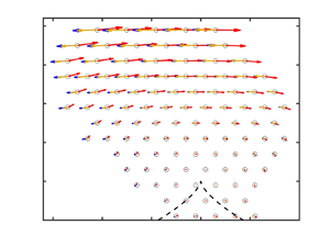
Figure 2. Joint p.d.f. of the dimensionless invariants  $\zeta$ and $\chi$ of the pressure Hessian conditioned on (a) $\varOmega \tau _K^2 = 1$, (b) $\varOmega \tau _K^2 = 4$, (c) $\varOmega \tau _K^2 = 25$ and (d) $\varOmega \tau _K^2 = 100$. The red line with cross symbols in (d) corresponds to a Burgers vortex. The white dashed-dotted lines show the iso-probability contours corresponding to the value $1$, and the dashed lines to $2^n$.
We now demonstrate that the structure of the p.d.f.s of  $(\zeta, \chi )$ conditioned on $\varOmega \tau _K^2 \gg 1$ is fully consistent with the presence of intense vortex tube-like structure (Siggia Reference Siggia1981; She et al. Reference She, Jackson and Orszag1990; Jiménez et al. Reference Jiménez, Wray, Saffman and Rogallo1993; Ishihara et al. Reference Ishihara, Gotoh and Kaneda2009; Buaria et al. Reference Buaria, Pumir, Bodenschatz and Yeung2019). To this end, we consider a Burgers vortex, characterized by the standard definition of the Reynolds number, $Re = \varGamma /\nu$, where $\varGamma$ is the circulation of the vortex. At the centre of the vortex (Burgers Reference Burgers1948) with $Re \gg 1$, the eigenvalues of the pressure Hessian are also $\frac {1}{4}\omega ^2$, $\frac {1}{4}\omega ^2$ and $0$; and the eigendirection corresponding to the $0$ eigenvalue aligns with $\hat {\boldsymbol {\omega }}$ (Andreotti Reference Andreotti1997; Horiuti Reference Horiuti2001; Horiuti & Takagi Reference Horiuti and Takagi2005). We now compare the structure of the pressure Hessian in a turbulent flow with that in a Burgers vortex, whose properties depend only on the distance $r$ to the axis. Following Andreotti (Reference Andreotti1997), we use the dimensionless radius $r^* = r \, a/\nu$, where $a$ is the external strain rate acting on the vortex. We note that the Reynolds number $Re$ amounts to the vorticity at the centre divided by the external strain $a$. As already stated, the maximum value of the probability in all panels of figure 2, indicated by the green squares, corresponds to the axisymmetric configuration on the axis of the vortex ( $r^* = 0$). Furthermore, the dependence of the invariants $\zeta$ and $\chi$ on $r^*$ up to $r^* = 1$ in a Burgers vortex is shown as the red line with crosses in figure 2(d), see also (4) of Andreotti (Reference Andreotti1997). As $r^*$ increases, the solution moves up in the $(\zeta, \chi )$ plane, first towards the left border and then back towards the centre. We note that its variation with respect to Reynolds number $Re$ is negligible. The joint p.d.f. of $(\zeta, \chi )$, particularly the ridges, closely follows the Burgers vortex solution. We also observe that when conditioning on a given value of $\varOmega \tau _K^2$, as done in figure 2, the points at a given value of $(\zeta, \chi )$ away from the maximum, or $\zeta = \chi = \sqrt {3}/9$, correspond to points at some distances away from the centre, or $r^* > 0$, of vortices with increasing intensity. These vortices are therefore less probable, which explains that the maximum probability in figure 2 corresponds to $\zeta = \chi = \sqrt {3}/9$. Additionally, the distribution becomes more concentrated along the red curve when $\varOmega \tau _K^2$ increases. Figure 2 therefore demonstrates that the Burgers vortex model provides a compelling qualitative description of the pressure Hessian. We notice, however, that any axisymmetric vortex model would lead to qualitatively similar observations near the centre of the vortex, consistent with (3.6) for the deviatoric part of the pressure Hessian tensor.
4. Dynamics in the  $(R,Q)$ plane

To illustrate the dynamical implications of (3.6), we project the equations of motion for  ${\boldsymbol{\mathsf{m}}}$ on the plane $(R,Q)$, where the invariants $R$ and $Q$ are defined by
 $$\begin{gather} Q \equiv-\tfrac{1}{2}{\mathsf{m}}_{ij}{\mathsf{m}}_{ji} =-\tfrac{1}{2} {{\mathsf{s}}}_{ij}{{\mathsf{s}}}_{ji} + \tfrac{1}{4} \omega^2, \end{gather}$$
 $$\begin{gather}R \equiv-\tfrac{1}{3}{\mathsf{m}}_{ij}{\mathsf{m}}_{jk}{\mathsf{m}}_{ki} =-\tfrac{1}{3} {{\mathsf{s}}}_{ij}{{\mathsf{s}}}_{jk} {{\mathsf{s}}}_{ki} - \tfrac{1}{4}\omega_i {{\mathsf{s}}}_{ij}\omega_j . \end{gather}$$
In (4.1) and (4.2), and throughout this text, we assume summation of repeated indices. Physically,  $Q$ expresses the difference between enstrophy and the square of the strain rate, so $Q = \frac {1}{2} \varOmega - {\rm tr}({\boldsymbol{\mathsf{s}}}^2) > 0$ corresponds to vorticity-dominated regions and $Q<0$ corresponds to strain-dominated regions. Similarly, $R = - \frac {1}{3} {\rm tr}({\boldsymbol{\mathsf{s}}}^2) - \frac {1}{4} \boldsymbol {\omega } \boldsymbol {\cdot } {\boldsymbol{\mathsf{s}}} \boldsymbol {\cdot } \boldsymbol {\omega } <0$ corresponds to the vortex-stretching-dominated region. The exact Lagrangian evolution equations for the invariants $R$ and $Q$ can be readily derived from (1.2):
 $$\begin{gather} \frac{{\rm d}Q}{{\rm d}t} =- 3 R + {\mathsf{m}}_{ij} {{\mathsf{H}}\,}^p_{ji} - {\mathsf{m}}_{ij} {{\mathsf{H}}}^\nu_{ji}, \end{gather}$$
 $$\begin{gather}\frac{{\rm d}R}{{\rm d}t} = \frac{2}{3} Q^2 + {\mathsf{m}}_{ij} {\mathsf{m}}_{jk} {{\mathsf{H}}\,}^p_{ki} - {\mathsf{m}}_{ij} {\mathsf{m}}_{jk} {{\mathsf{H}}}^\nu_{ki}, \end{gather}$$
where  ${{\mathsf{H}}\,}^p_{ij}$ is the deviatoric part of the pressure Hessian, and ${{\mathsf{H}}}^\nu _{ij} \equiv \nu ({\partial ^2 {\mathsf{m}}_{ij}}/{\partial x_k \partial x_k})$. We stress that these two terms in (4.3) and (4.4) are unclosed. The RE approximation introduced above provides a closure consisting in neglecting the deviatoric contributions to the pressure Hessian: ${\boldsymbol{\mathsf{H}}\kern0.7pt}^p = {\boldsymbol{\mathsf{0}}}$. As mentioned already (Buaria & Pumir Reference Buaria and Pumir2023), the RE assumption fails to predict the qualitative behaviour of the dynamics in the $(R,Q)$ plane when $Q$ is positive and large. Specifically, the RE assumption leads to ${{\rm d}R}/{{\rm d}t} = \frac {2}{3} Q^2 >0$, but the results of DNS show that ${{\rm d}R}/{{\rm d}t} < 0$ in some region of the second quadrant of the $(R, Q)$ plane, see, for example, figures 3(a) and 3(d) of Wilczek & Meneveau (Reference Wilczek and Meneveau2014) and figure 5 of Yang et al. (Reference Yang, Bodenschatz, He, Pumir and Xu2023). The observation that pressure leads to a ‘depression of nonlinearity’ (Borue & Orszag Reference Borue and Orszag1998) suggests the functional ${{\mathsf{H}}\,}^p_{ij} = - \alpha ({\mathsf{m}}_{ik}{\mathsf{m}}_{kj} - \frac {1}{3} {\rm tr}({\boldsymbol{\mathsf{m}}}^2)\delta _{ij})$ where $0 < \alpha < 1$ is a model parameter (Chertkov et al. Reference Chertkov, Pumir and Shraiman1999). This model predicts that the pressure terms induced by ${{\mathsf{H}}\,}^p_{ij}$ in (4.3) and (4.4) anti-align with the RE terms in the $(R,Q)$ plane, in quantitative contradiction with numerical results for $Q > 0$, and particularly for $R < 0$. Attempts to improve the RE approximation have assumed mostly some local expressions for the pressure Hessian, with an explicit relation between ${\boldsymbol{\mathsf{H}}\kern0.7pt}^p$ and the velocity gradient tensor ${\boldsymbol{\mathsf{m}}}$ (Wilczek & Meneveau Reference Wilczek and Meneveau2014). In the following, we will discuss theoretically the role of pressure Hessian in the vorticity-dominated regions, and derive a local analytical expression for the contributions of ${{\mathsf{H}}\,}^p_{ij}$ in Eqs. (4.3) and (4.4), to leading order when $\varOmega \tau _K^2 \gg 1$.
We now use the approximate form of the deviatoric part of the pressure Hessian, (3.6), to analyse the dynamics in the  $(R,Q)$ plane. When $\varOmega \tau _K^2 \gg 1$, (3.6) gives
 $$\begin{gather} {\mathsf{m}}_{ij} \tilde{H}^p_{ji} =-\tfrac{1}{4} \omega_i {{\mathsf{s}}}_{ij} \omega_j = R - \tfrac{1}{3}{{\mathsf{s}}}_{ij}{{\mathsf{s}}}_{jk}{{\mathsf{s}}}_{ki} , \end{gather}$$
 $$\begin{gather}{\mathsf{m}}_{ij}{\mathsf{m}}_{jk} \tilde{H}^p_{ki} =-\tfrac{2}{3} Q^2 - \tfrac{1}{12} \omega^2 {{\mathsf{s}}}_{ij}{{\mathsf{s}}}_{ji} +\tfrac{1}{6}({{\mathsf{s}}}_{ij} {{\mathsf{s}}}_{ji})^2 - \tfrac{1}{4} \omega_i {{\mathsf{s}}}_{ik}{{\mathsf{s}}}_{kj}\omega_j . \end{gather}$$
 We recall that the expressions for  ${\rm d}Q/{\rm d}t$ and ${\rm d}R/{\rm d}t$ obtained by using the RE approximation, provided by (4.3) and (4.4) are $- 3R$ and $\frac {2}{3} Q^2$, respectively. In the spirit of the approach in § 3.1, based on the quantitative difference between $\varSigma$ and $\varOmega$, namely with $\varSigma \ll \varOmega$ when $\varOmega \tau _K^2 \gg 1$, we further notice that when $\varOmega \tau _K^2 \gg 1$, $R \gg \frac {1}{3}{{\mathsf{s}}}_{ij}{{\mathsf{s}}}_{jk}{{\mathsf{s}}}_{ki}$, so the ${\boldsymbol{\mathsf{H}}\kern0.7pt}^p$ term cancels, to the leading order in $\varSigma /\varOmega$, approximately $1/3$ of the RE term in the $Q$ equation. More significantly, in the limit $\varOmega \tau _K^2 \gg 1$, we find that $Q^2 \gg \omega ^2 {{\mathsf{s}}}_{ij}{{\mathsf{s}}}_{ji}, \omega _i {{\mathsf{s}}}_{ik}{{\mathsf{s}}}_{kj}\omega _j \gg ({{\mathsf{s}}}_{ij} {{\mathsf{s}}}_{ji})^2$ in the $R$ equation, so the ${\boldsymbol{\mathsf{H}}\kern0.7pt}^p$ terms cancel out the dominant RE term $\frac {2}{3} Q^2$. The lowest-order contribution in a formal development in $(\varSigma /\varOmega )$ involves terms such as $- \frac {1}{12} \omega ^2 {{\mathsf{s}}}_{ij}{{\mathsf{s}}}_{ji} - \frac {1}{4} \omega _i {{\mathsf{s}}}_{ik}{{\mathsf{s}}}_{kj}\omega _j$, which is negative. We observe that this implies ${\rm d}R/{\rm d}t < 0$, which is generally consistent with the DNS results (see e.g. figure 5 of Yang et al. Reference Yang, Bodenschatz, He, Pumir and Xu2023). Earlier work aimed at describing the pressure Hessian (Chevillard et al. Reference Chevillard, Meneveau, Biferale and Toschi2008; Wilczek & Meneveau Reference Wilczek and Meneveau2014) did not particularly focus on high-enstrophy regions. It would be interesting to compare the corresponding predictions in light of the approximation. We note that the tetrad model (Chertkov et al. Reference Chertkov, Pumir and Shraiman1999; Yang et al. Reference Yang, Pumir and Xu2020, Reference Yang, Bodenschatz, He, Pumir and Xu2023) involves quadratic terms in the vorticity introduced through the full tensor ${\boldsymbol{\mathsf{m}}}$, insufficient to compensate for the strong vortex-stretching reduction due to the RE approximation.
Figure 3(a) shows the DNS results for  ${{\rm d}Q}/{{\rm d}t}$ and ${{\rm d}R}/{{\rm d}t}$ on the $(R,Q)$ plane (blue arrows) and compares them with the theoretical predictions (magenta arrows). Figure 3(a) demonstrates that when $Q \tau _K^2 \gtrsim 5$ and $|R \, \tau _K^3|$ is not too large, the magenta arrows, which represent our theoretical predictions (rightmost terms of (4.5), (4.6)), agree well with the blue arrows, which represent the ‘exact’ DNS values. Figure 3 also directly compares the ratios between the numerically determined values ${\rm tr}({\boldsymbol{\mathsf{H}}\kern0.7pt}^p \boldsymbol {\cdot } {\boldsymbol{\mathsf{m}}} )$ (b) and ${\rm tr}({\boldsymbol{\mathsf{H}}\kern0.7pt}^p \boldsymbol {\cdot } {\boldsymbol{\mathsf{m}}}^2 )$ (c) and the values found by replacing ${\boldsymbol{\mathsf{H}}\kern0.7pt}^p$ by $\tilde {{\boldsymbol{\mathsf{H}}}\kern0.7pt}^p$. The agreement for the ${\rm tr}({\boldsymbol{\mathsf{H}}\kern0.7pt}^p \boldsymbol {\cdot } {\boldsymbol{\mathsf{m}}}^2 )$ generally improves when $Q$ increases, as expected when $\varOmega \tau _K^2$ increases. The effect is weaker for the term ${\rm tr}({\boldsymbol{\mathsf{H}}\kern0.7pt}^p \boldsymbol {\cdot } {\boldsymbol{\mathsf{m}}})$. We note that the quality of the agreement at $R \approx 0$ degrades when $Q \tau _K^2$ increases, which is due to the small values of both numerator and denominator. Figure 4 provides further insight on the dynamics, by comparing the contributions of ${\boldsymbol{\mathsf{H}}\kern0.7pt}^p$ to ${{\rm d}Q}/{{\rm d}t}$ and ${{\rm d}R}/{{\rm d}t}$ in the $(R,Q)$ plane, with the leading-order terms in (4.5) and (4.6), namely $R$ and $- \frac {2}{3} Q^2$. Figure 4 reveals that when $Q \tau _K^2 > 5$ and $|R\tau _K^3|$ is not too large, the green arrows, which represent our theoretical predictions to leading order are reassuringly close to the blue arrows, which represent the values obtained directly from DNS.

Figure 3. (a) Results for  ${{\rm d}Q}/{{\rm d}t}$ and ${{\rm d}R}/{{\rm d}t}$ in the $(R,Q)$ plane. The red arrows show the RE term $(-3R, \frac {2}{3}Q^2)$, the blue arrows the deviatoric pressure Hessian term $(- {\mathsf{m}}_{ij} {{\mathsf{H}}\,}^p_{ji}, - {\mathsf{m}}_{ij}{\mathsf{m}}_{jk} {{\mathsf{H}}\,}^p_{ki})$ and the magenta arrows our theoretical predictions for large $\varOmega$, i.e. the rightmost terms of (4.5), (4.6). Panels (b,c) show the ratio between the contributions of the deviatoric part of the pressure Hessian, ${\boldsymbol{\mathsf{H}}\kern0.7pt}^p$, and those of the approximate form, $\tilde {{\boldsymbol{\mathsf{H}}}\kern0.7pt}^p$, (3.6), to ${\rm d} Q/{\rm d}t$ (b) and ${\rm d}R/{\rm d}t$ (c). The ratios, plotted as a function of $R \tau _K^3$, increase towards $1$ as $Q \tau _K^2$ increases. The large value for ${\rm d}Q/{\rm d}t$ close to $R \tau _K^3 \approx 0$ corresponds to very small values of both the terms ${\rm tr}({\boldsymbol{\mathsf{H}}\kern0.7pt}^p \boldsymbol {\cdot } {\boldsymbol{\mathsf{m}}})$ and ${\rm tr}(\tilde {{\boldsymbol{\mathsf{H}}}\kern0.7pt}^p \boldsymbol {\cdot } {\boldsymbol{\mathsf{m}}})$. Dataset B was used to construct the figure.

Figure 4. (a) Pressure contribution to  ${{\rm d}Q}/{{\rm d}t}$ and ${{\rm d}R}/{{\rm d}t}$ in the $(R,Q$) plane. The red arrows correspond to the RE term $(-3R, \frac {2}{3}Q^2)$, which corresponds to the isotropic (local) contribution of the pressure Hessian, the blue arrows to the anisotropic pressure Hessian term $(- {\mathsf{m}}_{ij} H^p_{ji}, - {\mathsf{m}}_{ij}{\mathsf{m}}_{jk} H^p_{ki})$ and the green arrows show the simplified theoretical predictions at large $\varOmega$, $(R, -\frac {2}{3}Q^2)$. Panel (b) shows the ratio between the contribution of ${\boldsymbol{\mathsf{H}}\kern0.7pt}^p$ to ${\rm d}R/{\rm d}t$, compared with the simplified form $-2 Q^2/3$. Dataset B ( $R_\lambda = 210$) was used to construct the figure.
Remarkably, we notice that using  $-\frac {2}{3} Q^2$ for the contribution due to the deviatoric part of the pressure Hessian leads to ${\rm d}R/{\rm d}t = 0$ in the inviscid case. Whether the blue arrows in figure 4(a) are longer or shorter than the green ones in fact determines the sign of ${\rm d}R/{\rm d}t$. We observe that ${\rm d}R/{\rm d}t > 0$ when $Q \tau _K^2 \gtrsim 20$ for Dataset B with $R_\lambda = 210$. At lower values of $Q \tau _K^2$, and for $R \tau _K^3$ sufficiently negative, on the contrary, ${\rm d}R/{\rm d}t < 0$. For these values, the dynamics tends to keep the values $(R,Q)$ in the ( $R < 0, Q > 0$) quadrant, where stretching is largest. This contrasts sharply with the predictions of the RE approximation, which tends to inhibit vortex stretching (Buaria & Pumir Reference Buaria and Pumir2023). A more precise comparison between ${\rm tr}( {\boldsymbol{\mathsf{H}}\kern0.7pt}^p \boldsymbol {\cdot } {\boldsymbol{\mathsf{m}}}^2)$ and $-\frac {2}{3} Q^2$ is shown in figure 4(b). At relatively low value of $Q \tau _K^2$, and for $R \tau _K^3 \lesssim -3$, ${\rm tr} ({\boldsymbol{\mathsf{H}}\kern0.7pt}^p \boldsymbol {\cdot } {\boldsymbol{\mathsf{m}}}^2 )$ is more negative than $-\frac {2}{3} Q^2$, consistent with the observation that ${\rm d}R/{\rm d}t < 0$. As $Q \tau _K^2$ increases, however, the region where ${\rm d}R/{\rm d}t < 0$ is restricted to much larger values of $R \tau _K^3 < 0$, whereas at small, intermediate values of $|R\tau_K^3|$, ${\rm d}R/{\rm d}t > 0$.
5. Conclusion
In this work, we have proposed a very simple approximate expression for the deviatoric part of the pressure Hessian in terms of the local field, valid in regions of very large vorticity in turbulent flows. Namely, we find that  ${\partial ^2 p}/{\partial x_i \partial x_j} \sim - \frac {1}{4}(\omega _i \omega _j - \omega ^2 \delta _{ij} )$ when $\omega ^2 \tau _K^2 \gg 1$. This simple expression comes from an elementary analysis of the flow, and in particular, on the structure of the solutions (vortex tubes) in these flow regions. We stress that the deviatoric term of the pressure Hessian is essentially non-local, which implies that (3.6) can be only approximately valid. Despite these limitations, the observations from DNS support our theoretical discussions and provide further evidence for our conclusions. The numerical results in homogeneous isotropic flows presented here therefore demonstrate that the considerations developed in this work provide potentially valuable insight into the closure models of pressure Hessian in the Lagrangian dynamics of velocity gradient. Although one expects on general grounds that our conclusions should extend to other turbulent flows, e.g. in the presence of mean shear and/or walls at large Reynolds numbers, it will be interesting to check the validity of our approximation for other classes of turbulent flows.
The expression (3.6) reduces to the simple explicit (local) relation between  $\tilde {{\boldsymbol{\mathsf{H}}}\kern0.7pt}^p_{ij}$ and ${{\mathsf{w}}}_{ij} \equiv \frac {1}{2}({\mathsf{m}}_{ij} - {\mathsf{m}}_{ji})$, the antisymmetric part of the velocity gradient tensor: $\tilde {{{\mathsf{H}}}\,}^p_{ij} = {{\mathsf{w}}}_{ik} {{\mathsf{w}}}_{kj} - \frac {1}{3} {\rm tr}({\boldsymbol{\mathsf{w}}}^2)\delta _{ij}$. We note in this respect that recent machine-learning approaches (Tian et al. Reference Tian, Livescu and Chertkov2021; Buaria & Sreenivasan Reference Buaria and Sreenivasan2023) have looked systematically for an expansion of ${\boldsymbol{\mathsf{H}}\kern0.7pt}^p$ in terms of all the invariants of the velocity gradient tensor, ${\boldsymbol{\mathsf{m}}}$. In this sense, (3.6) can be compared with that from machine learning approaches. Alternatively, the expression provides a point of comparison which may be used in a physics-informed machine-learning approach. It is our expectation that the physical considerations initiated in this work can be further developed, and can lead to clearer understanding of the structure and modelling of turbulent flows.
Funding
P.-F.Y., H.X. and G.W.H. are grateful to the Natural Science Foundation of China (NSFC) Basic Science Center Program ‘Multiscale Problems in Nonlinear Mechanics’ (grant no. 11988102). P.-F.Y. and H.X. also acknowledge financial support from the NSFC grants 12202452, 11672157 and 91852104. A.P. received support from Agence Nationale de la Recherche (ANR) under grant number Contract TILT No. ANR-20-CE30-0035.
Declaration of interests
The authors report no conflict of interest.


 Open access