


1 Introduction
Geophysical vortices, such as those in the atmosphere and oceans, are observed in a dynamical state that often departs, if only slightly, from a symmetric flow rotating around a vertically oriented axis (for example, Boulanger, Meunier & Le Dizès Reference Boulanger, Meunier and Le Dizès2007). Hence, a classical set of problems in physical oceanography and dynamical meteorology deals with the processes of horizontal axisymmetrization and vertical alignment of baroclinic vortices (for example, Viera Reference Viera1995; Schecter, Montgomery & Reasor Reference Schecter, Montgomery and Reasor2002). In particular, the initial tilt of a geophysical vortex may be due either to its initial vortex genesis (Canals, Pawlak & MacCready Reference Canals, Pawlak and MacCready2009) or to the action of any external forcing (for example, Tang et al. Reference Tang, Gulick, Sun, Sun and Jing2020). Our understanding of the vertical alignment of vortices could be substantially improved with a mathematical model able to describe in a simple way the permanent precession of vortices with distributed potential vorticity anomaly. This work provides, under the quasi-geostrophic (QG) approximation, a vortex model with distributed potential vorticity able to sustain, under inviscid and adiabatic conditions, a permanent precession of its vertical axis.
The basic QG dynamics required to describe the precessing vortex model is first briefly introduced in § 2, including the fundamental equation expressing the material conservation of QG potential vorticity anomaly  $\unicode[STIX]{x1D71B}(\boldsymbol{x},t)$ (PVA) by the horizontal geostrophic flow $\boldsymbol{u}(\boldsymbol{x},t)$. In the next section § 3 we introduce a PVA distribution $\widetilde{\unicode[STIX]{x1D71B}}(\boldsymbol{x},t_{0})$ at the initial time, say, $t_{0}=0$, involving only three modes, comprising spherical Bessel functions of the first kind $\text{j}_{l}(\unicode[STIX]{x1D70C})$, and spherical harmonics $\text{Y}_{l}^{m}(\unicode[STIX]{x1D703},\unicode[STIX]{x1D711})$, where $(\unicode[STIX]{x1D70C},\unicode[STIX]{x1D703},\unicode[STIX]{x1D711})$ are the spherical coordinates. The modes used are the spherical zero-degree mode $\hat{\unicode[STIX]{x1D71B}}_{0}\text{j}_{0}(\unicode[STIX]{x1D70C})$, and the second-degree modes $\hat{\unicode[STIX]{x1D71B}}_{2,0}\text{j}_{2}(\unicode[STIX]{x1D70C})\text{Y}_{2}^{0}(\unicode[STIX]{x1D703})$ and $\hat{\unicode[STIX]{x1D71B}}_{2,1}\text{j}_{2}(\unicode[STIX]{x1D70C})\text{Y}_{2}^{1}(\unicode[STIX]{x1D703},\unicode[STIX]{x1D711})$. It is postulated that this PVA distribution $\widetilde{\unicode[STIX]{x1D71B}}(\boldsymbol{x},t_{0})$ evolves, subjected to the QG dynamics, as a stable precessing vortex as long as the modal amplitudes $|\hat{\unicode[STIX]{x1D71B}}_{2,0}|$ and $|\hat{\unicode[STIX]{x1D71B}}_{2,1}|$ are smaller than the spherical vortex amplitude $|\hat{\unicode[STIX]{x1D71B}}_{0}|$ (that is, as long as the modes of degree 2 are small perturbations to the spherical mode). The stable precession is verified using three-dimensional numerical simulations. Then a closed-form PVA field $\tilde{\unicode[STIX]{x1D71B}}(\boldsymbol{x},t)$ is obtained in § 4 as an approximate solution to the unsteady $\widetilde{\unicode[STIX]{x1D71B}}(\boldsymbol{x},t)$. This approximate solution $\tilde{\unicode[STIX]{x1D71B}}(\boldsymbol{x},t)$ is periodic but not rigid, and addresses both the precession frequency and precession axis slope of the vortex. Finally, concluding remarks are given in § 5.
2 Basic QG dynamics
The inviscid adiabatic QG flow is governed by the conservation of QG PVA  $\unicode[STIX]{x1D71B}(\boldsymbol{x},t)$,
 $$\begin{eqnarray}{\displaystyle \frac{\text{d}_{g}\unicode[STIX]{x1D71B}}{\text{d}t}}\equiv {\displaystyle \frac{\unicode[STIX]{x2202}\unicode[STIX]{x1D71B}}{\unicode[STIX]{x2202}t}}+\boldsymbol{u}\boldsymbol{\cdot }\unicode[STIX]{x1D735}_{h}\unicode[STIX]{x1D71B}=0\end{eqnarray}$$
 by the horizontal geostrophic flow  $\boldsymbol{u}(\boldsymbol{x},t)\equiv -\unicode[STIX]{x1D735}_{h}\times (\unicode[STIX]{x1D719}\boldsymbol{e}_{z})$, scaled by $f_{0}^{-1}$, where $f_{0}$ is the constant background vorticity, or Coriolis parameter, and $\unicode[STIX]{x1D719}(\boldsymbol{x},t)$ is the geopotential anomaly field. The QG PVA $\unicode[STIX]{x1D71B}(\boldsymbol{x},t)$ is the sum of the dimensionless (scaled by $f_{0}^{-1}$) vertical component of geostrophic vorticity $\unicode[STIX]{x1D701}(\boldsymbol{x},t)=\unicode[STIX]{x1D6FB}_{h}^{2}\unicode[STIX]{x1D719}$ and the dimensionless vertical stratification anomaly ${\mathcal{S}}(\boldsymbol{x},t)=-\unicode[STIX]{x2202}{\mathcal{D}}(\boldsymbol{x},t)/\unicode[STIX]{x2202}z=\unicode[STIX]{x2202}^{2}\unicode[STIX]{x1D719}/\unicode[STIX]{x2202}\hat{z}^{2}$, where ${\mathcal{D}}$ is the vertical displacement of isopycnals. Above $\hat{z}\equiv (N_{0}/f_{0})z$, where $N_{0}$ is the constant background Brunt–Väisälä frequency. Henceforth we omit the hat symbol ( $\hat{\hspace{2.22198pt}\hspace{2.22198pt}}$) in $\hat{z}$ and will always work in the QG space, now simply denoted as $(x,y,z)$. The QG PVA $\unicode[STIX]{x1D71B}$ equals, in the vertically stretched QG space $(x,y,z)$, the Laplacian of $\unicode[STIX]{x1D719}(\boldsymbol{x},t)$,
 $$\begin{eqnarray}\unicode[STIX]{x1D71B}=\unicode[STIX]{x1D701}+{\mathcal{S}}=\unicode[STIX]{x1D6FB}^{2}\unicode[STIX]{x1D719}.\end{eqnarray}$$
 In terms of the geopotential  $\unicode[STIX]{x1D719}(\boldsymbol{x},t)$ the QG PVA conservation (2.1) is
 $$\begin{eqnarray}{\displaystyle \frac{\unicode[STIX]{x2202}}{\unicode[STIX]{x2202}t}}\unicode[STIX]{x1D6FB}^{2}\unicode[STIX]{x1D719}+(\boldsymbol{e}_{z}\times \unicode[STIX]{x1D735}_{h}\unicode[STIX]{x1D719})\boldsymbol{\cdot }\unicode[STIX]{x1D735}_{h}\unicode[STIX]{x1D6FB}^{2}\unicode[STIX]{x1D719}={\displaystyle \frac{\unicode[STIX]{x2202}}{\unicode[STIX]{x2202}t}}\unicode[STIX]{x1D6FB}^{2}\unicode[STIX]{x1D719}+{\mathcal{J}}\{\unicode[STIX]{x1D719},\unicode[STIX]{x1D6FB}^{2}\unicode[STIX]{x1D719}\}=0,\end{eqnarray}$$
 where  ${\mathcal{J}}\{A,B\}\equiv \unicode[STIX]{x2202}A/\unicode[STIX]{x2202}x\unicode[STIX]{x2202}B/\unicode[STIX]{x2202}y-\unicode[STIX]{x2202}A/\unicode[STIX]{x2202}y\unicode[STIX]{x2202}B/\unicode[STIX]{x2202}x$ is the Jacobian operator. Steady-state solutions to (2.3), with separation of variables in spherical coordinates $(\unicode[STIX]{x1D70C},\unicode[STIX]{x1D703},\unicode[STIX]{x1D711})$ and regular at the origin, are the product of the spherical Bessel functions of the first kind $\text{j}_{l}(\unicode[STIX]{x1D70C})$ with the spherical harmonics $\text{Y}_{l}^{m}(\unicode[STIX]{x1D703},\unicode[STIX]{x1D711})$, of degree $l$ and order $m$, which satisfy the Helmholtz equation $\unicode[STIX]{x1D6FB}^{2}(\,\text{j}_{l}(\unicode[STIX]{x1D70C})\text{Y}_{l}^{m}(\unicode[STIX]{x1D703},\unicode[STIX]{x1D711}))=-\text{j}_{l}(\unicode[STIX]{x1D70C})\text{Y}_{l}^{m}(\unicode[STIX]{x1D703},\unicode[STIX]{x1D711})$. These solutions, with distributed PVA, are used to describe the precessing QG vortex in the next section.
3 The three modes vertically precessing QG vortex
In this section we describe the precessing QG vortex directly from the initial QG PVA distribution  $\widetilde{\unicode[STIX]{x1D71B}}(\boldsymbol{x},t_{0})$. The purpose is to show that, for some range of the modal vortex amplitudes, this initial condition leads to a stable precessing vortex. Those readers already familiar with the QG PV dynamics will rapidly understand the vortex precession directly from the geometry of the modal components of the vortex configuration. The more rigorous mathematical justification of this vortex configuration is postponed to the next section.
The vortex interior comprises three PVA modes, consisting of simple spherical Bessel and spherical harmonics modes, defined as
 $$\begin{eqnarray}\displaystyle & \unicode[STIX]{x1D71B}_{0}(\unicode[STIX]{x1D70C})\equiv \hat{a}_{0}(\,\text{j}_{0}(\unicode[STIX]{x1D70C})-\text{j}_{0}(\unicode[STIX]{x1D70C}_{1}))\text{Y}_{0}^{0}=\hat{\unicode[STIX]{x1D71B}}_{0}(\,\text{j}_{0}(\unicode[STIX]{x1D70C})-\text{j}_{0}(\unicode[STIX]{x1D70C}_{1})), & \displaystyle\end{eqnarray}$$
 $$\begin{eqnarray}\displaystyle & \unicode[STIX]{x1D71B}_{2,0}(\unicode[STIX]{x1D70C},\unicode[STIX]{x1D703})\equiv \hat{a}_{2,0}\text{j}_{2}(\unicode[STIX]{x1D70C})\text{Y}_{2}^{0}(\unicode[STIX]{x1D703})=\hat{\unicode[STIX]{x1D71B}}_{2,0}\text{j}_{2}(\unicode[STIX]{x1D70C})(3\cos ^{2}\unicode[STIX]{x1D703}-1), & \displaystyle\end{eqnarray}$$
 $$\begin{eqnarray}\displaystyle & \unicode[STIX]{x1D71B}_{2,1}(\unicode[STIX]{x1D70C},\unicode[STIX]{x1D703},\unicode[STIX]{x1D711})\equiv \hat{a}_{2,1}\text{j}_{2}(\unicode[STIX]{x1D70C})\text{Y}_{2}^{1}(\unicode[STIX]{x1D703},\unicode[STIX]{x1D711})=\hat{\unicode[STIX]{x1D71B}}_{2,1}\text{j}_{2}(\unicode[STIX]{x1D70C})\sin \unicode[STIX]{x1D703}\cos \unicode[STIX]{x1D703}\cos \unicode[STIX]{x1D711}. & \displaystyle\end{eqnarray}$$
 The PVA modes are defined here as real-valued functions so that the complex modal amplitude  $\hat{a}_{2,1}$ is such that $\hat{\unicode[STIX]{x1D71B}}_{2,1}$ is a real-valued amplitude. The normalization constants of the spherical harmonics are absorbed in the modal PVA amplitudes. To use modal PVA amplitudes independent of the spherical harmonic normalization, constants $\{\hat{\unicode[STIX]{x1D71B}}_{0},\hat{\unicode[STIX]{x1D71B}}_{2,0},\hat{\unicode[STIX]{x1D71B}}_{2,1}\}$ must be replaced with $\{(1/2\sqrt{\unicode[STIX]{x03C0}})\hat{\unicode[STIX]{x1D71B}}_{0},{\textstyle \frac{1}{4}}\sqrt{(5/\unicode[STIX]{x03C0})}\hat{\unicode[STIX]{x1D71B}}_{2,0},-{\textstyle \frac{1}{2}}\sqrt{(15/2\unicode[STIX]{x03C0})}\hat{\unicode[STIX]{x1D71B}}_{2,1}\}$.
The precessing vortex is defined as a piecewise PVA function with three subdomains,
 $$\begin{eqnarray}\widetilde{\unicode[STIX]{x1D71B}}(\unicode[STIX]{x1D70C},\unicode[STIX]{x1D703},\unicode[STIX]{x1D711},t_{0})\equiv \left\{\begin{array}{@{}ll@{}}\unicode[STIX]{x1D71B}_{0}(\unicode[STIX]{x1D70C})+\unicode[STIX]{x1D71B}_{2,0}(\unicode[STIX]{x1D70C},\unicode[STIX]{x1D703})+\unicode[STIX]{x1D71B}_{2,1}(\unicode[STIX]{x1D70C},\unicode[STIX]{x1D703},\unicode[STIX]{x1D711}),\quad & \unicode[STIX]{x1D70C}\leqslant \unicode[STIX]{x1D70C}_{1}\\ \unicode[STIX]{x1D71B}_{2,0}(\unicode[STIX]{x1D70C},\unicode[STIX]{x1D703})+\unicode[STIX]{x1D71B}_{2,1}(\unicode[STIX]{x1D70C},\unicode[STIX]{x1D703},\unicode[STIX]{x1D711}),\quad & \unicode[STIX]{x1D70C}_{1}<\unicode[STIX]{x1D70C}\leqslant \unicode[STIX]{x1D70C}_{2}\\ 0,\quad & \unicode[STIX]{x1D70C}_{2}<\unicode[STIX]{x1D70C}.\end{array}\right.\end{eqnarray}$$
 The three subdomains are spherical shells (for brevity referred to here as the inner, intermediate or transition, and outer domains) defined from the first zeros,  $\unicode[STIX]{x1D70C}_{1}$ and $\unicode[STIX]{x1D70C}_{2}$, of the spherical Bessel functions $\text{j}_{1}(\unicode[STIX]{x1D70C})$ and $\text{j}_{2}(\unicode[STIX]{x1D70C})$ (that is, $\text{j}_{1}(\unicode[STIX]{x1D70C}_{1})=0$ and $\text{j}_{2}(\unicode[STIX]{x1D70C}_{2})=0$). Because of their frequent use here we record the constants
 $$\begin{eqnarray}\unicode[STIX]{x1D70C}_{1}\simeq 4.493,\quad \unicode[STIX]{x1D70C}_{2}\simeq 5.763,\quad \text{j}_{0}(\unicode[STIX]{x1D70C}_{1})\simeq -0.2172\quad \text{and}\quad \text{j}_{0}(\unicode[STIX]{x1D70C}_{2})\simeq -0.08617.\quad\end{eqnarray}$$
 Mode  $\unicode[STIX]{x1D71B}_{0}(\unicode[STIX]{x1D70C})$, having radial $\unicode[STIX]{x1D70C}$ symmetry, is the spherical mode, or unperturbed vortex. Since $\unicode[STIX]{x1D71B}_{0}(\unicode[STIX]{x1D70C})$ has no particular axis of symmetry (all the radial axes are axes of symmetry), all the rotations leave the PVA mode invariant, and therefore it is not a mode susceptible to being tilted. Mode $\unicode[STIX]{x1D71B}_{0}(\unicode[STIX]{x1D70C})$ occupies only the inner vortex, vanishing at the radius $\unicode[STIX]{x1D70C}_{1}$ where $\text{j}_{0}^{\prime }(\unicode[STIX]{x1D70C}_{1})=\text{j}_{1}(\unicode[STIX]{x1D70C}_{1})=0$, and therefore $\unicode[STIX]{x1D71B}_{0}(\unicode[STIX]{x1D70C}_{1})=\unicode[STIX]{x1D71B}_{0}^{\prime }(\unicode[STIX]{x1D70C}_{1})=0$.
Modes  $\unicode[STIX]{x1D71B}_{2,0}(\unicode[STIX]{x1D70C},\unicode[STIX]{x1D703})$ and $\unicode[STIX]{x1D71B}_{2,1}(\unicode[STIX]{x1D70C},\unicode[STIX]{x1D703},\unicode[STIX]{x1D711})$ occupy both the inner and intermediate domains, since they terminate at the radius $\unicode[STIX]{x1D70C}_{2}$ where $\unicode[STIX]{x1D71B}_{2,0}(\unicode[STIX]{x1D70C}_{2},\unicode[STIX]{x1D703})=\unicode[STIX]{x1D71B}_{2,1}(\unicode[STIX]{x1D70C}_{2},\unicode[STIX]{x1D703},\unicode[STIX]{x1D711})=0$. Mode $\unicode[STIX]{x1D71B}_{2,0}(\unicode[STIX]{x1D70C},\unicode[STIX]{x1D703})$ (figure 1a) is the zonal vortex mode, symmetric around its vertical axis (has no azimuthal $\unicode[STIX]{x1D711}$ dependence), and therefore is susceptible to being tilted. By itself, mode $\unicode[STIX]{x1D71B}_{2,0}(\unicode[STIX]{x1D70C},\unicode[STIX]{x1D703})$ is centrifugally unstable (for example, Sipp & Jacquin Reference Sipp and Jacquin2000), since the PVA gradient $\unicode[STIX]{x1D735}\unicode[STIX]{x1D71B}_{2,0}$ changes sign within its domain. However, the spherical mode $\unicode[STIX]{x1D71B}_{0}(\unicode[STIX]{x1D70C})$ can stabilize the vortex, at least within its inner domain, as long as the spherical modal amplitude satisfies $|\hat{\unicode[STIX]{x1D71B}}_{0}|\gg |\hat{\unicode[STIX]{x1D71B}}_{2,0}|$.

Figure 1. Isosurfaces of the PVA modes. Isosurfaces of (a)  $\unicode[STIX]{x1D71B}_{2,0}(\boldsymbol{x})=\pm 1$, (b) $\unicode[STIX]{x1D71B}_{2,1}(\boldsymbol{x})=\pm 1$ and (c) $\unicode[STIX]{x1D71B}_{2,0}(\boldsymbol{x})+\unicode[STIX]{x1D71B}_{2,1}(\boldsymbol{x})=\pm 1$. Modal amplitudes $\hat{\unicode[STIX]{x1D71B}}_{2,0}=\hat{\unicode[STIX]{x1D71B}}_{2,1}=1$. Blue colour means negative values and orange colour means positive values.
Mode  $\unicode[STIX]{x1D71B}_{2,1}(\unicode[STIX]{x1D70C},\unicode[STIX]{x1D703},\unicode[STIX]{x1D711})$ (figure 1b) is, by itself, baroclinically unstable or, better expressed, is the baroclinic instability, in the sense that it consists of two baroclinic dipoles, one above the other, travelling horizontally in opposite directions along straight trajectories. These baroclinic dipoles would experience vertical shear since, for symmetry reasons, the flow velocity vanishes at the mid-depth $z=0$. However, the vortex may be stable due to, again, the addition of the spherical mode $\unicode[STIX]{x1D71B}_{0}(\unicode[STIX]{x1D70C})$, which adds curvature to the $\unicode[STIX]{x1D71B}_{2,1}$ dipole trajectories, as occurs with the radial and dipolar modes in the two-dimensional Chaplygin–Lamb vortex (Chaplygin Reference Chaplygin1903; Flierl, Stern & Whitehead Reference Flierl, Stern and Whitehead1983; Meleshko & van Heijst Reference Meleshko and van Heijst1994), or as happens with the spherical and dipolar modes, which depend on $\text{j}_{0}(\unicode[STIX]{x1D70C})$ and $\text{j}_{1}(\unicode[STIX]{x1D70C})\text{Y}_{1}^{1}(\unicode[STIX]{x1D703},\unicode[STIX]{x1D711})$ in baroclinic QG dipoles (Viúdez Reference Viúdez2019). If this curvature radius is much smaller than the vortex radius (roughly if $z|\hat{\unicode[STIX]{x1D71B}}_{2,1}|/|\hat{\unicode[STIX]{x1D71B}}_{0}|\ll z\unicode[STIX]{x1D70C}_{2}$ – that is, if $|\hat{\unicode[STIX]{x1D71B}}_{0}|\gg |\hat{\unicode[STIX]{x1D71B}}_{2,1}|$), the inner vortex remains stable and oscillates due to the presence of the two dipoles of the $\unicode[STIX]{x1D71B}_{2,1}$ mode.
The specification of the PVA in the intermediate transition domain shell  $\unicode[STIX]{x1D70C}_{1}<\unicode[STIX]{x1D70C}<\unicode[STIX]{x1D70C}_{2}$ is not, however, unique. Several possibilities, different from that in (3.4), seem to be possible. Extending the mode-0 domain to $\unicode[STIX]{x1D70C}\leqslant \unicode[STIX]{x1D70C}_{2}$ is another option; although in this case the spherical mode becomes unstable in the intermediate region $\unicode[STIX]{x1D70C}_{1}<\unicode[STIX]{x1D70C}\leqslant \unicode[STIX]{x1D70C}_{2}$, since the gradient of $\text{j}_{0}(\unicode[STIX]{x1D70C})$ changes sign at $\unicode[STIX]{x1D70C}=\unicode[STIX]{x1D70C}_{1}$. Another option is to stretch the radial variable of the spherical Bessel function $\text{j}_{0}(k_{0}\,\unicode[STIX]{x1D70C})$, with $k_{0}\equiv \unicode[STIX]{x1D70C}_{1}/\unicode[STIX]{x1D70C}_{2}$, and extend the inner domain to $\unicode[STIX]{x1D70C}\leqslant \unicode[STIX]{x1D70C}_{2}$, so that $\text{j}_{0}(k_{0}\,\unicode[STIX]{x1D70C}_{2})=\text{j}_{0}(\unicode[STIX]{x1D70C}_{1})$. However, in this case the vortex becomes unsteady in the inner domain $\unicode[STIX]{x1D70C}\leqslant \unicode[STIX]{x1D70C}_{2}$, since the advective cross-terms of modes $\{0\}$ and $\{2,1\}$ no longer cancel out (that is, ${\mathcal{J}}\{\unicode[STIX]{x1D719}_{0},\unicode[STIX]{x1D6FB}^{2}\unicode[STIX]{x1D719}_{2,1}\}+{\mathcal{J}}\{\unicode[STIX]{x1D719}_{2,1},\unicode[STIX]{x1D6FB}^{2}\unicode[STIX]{x1D719}_{0}\}=-{\mathcal{J}}\{\unicode[STIX]{x1D719}_{0},\unicode[STIX]{x1D719}_{2,1}\}-k_{0}^{2}{\mathcal{J}}\{\unicode[STIX]{x1D719}_{2,1},\unicode[STIX]{x1D719}_{0}\}=(k_{0}^{2}-1){\mathcal{J}}\{\unicode[STIX]{x1D719}_{0},\unicode[STIX]{x1D719}_{2,1}\}$). Thus we have used (3.4) as the least unsteady among the different possibilities considered (being aware, however, that other solutions may be possible).
It rests now to prove that for small amplitudes  $|\hat{\unicode[STIX]{x1D71B}}_{2,1}|$, such that the ratio $|\hat{\unicode[STIX]{x1D71B}}_{2,0}/\hat{\unicode[STIX]{x1D71B}}_{2,1}|=|\unicode[STIX]{x1D716}_{0}|\ll 1$, the addition of modes $\unicode[STIX]{x1D71B}_{2,0}$ and $\unicode[STIX]{x1D71B}_{2,1}$ is approximately equal to a rotation of $\unicode[STIX]{x1D71B}_{2,0}$ around an horizontal axis (figure 1c). First we write, using a convenient mix of spherical, cylindrical $(r,\unicode[STIX]{x1D717},z)$, and Cartesian $(x,y,z)$ coordinates, $\unicode[STIX]{x1D71B}_{2,0}=\hat{\unicode[STIX]{x1D719}}_{2,0}\text{j}_{2}(\unicode[STIX]{x1D70C})(2z^{2}-r^{2})/\unicode[STIX]{x1D70C}^{2}$ and $\unicode[STIX]{x1D71B}_{2,1}=\hat{\unicode[STIX]{x1D719}}_{2,1}\text{j}_{2}(\unicode[STIX]{x1D70C})xz/\unicode[STIX]{x1D70C}^{2}$. Since a rotation around the $y$-axis by a small angle $|\unicode[STIX]{x1D6FC}_{0}|\ll 1$ transforms $(x,y,z)\rightarrow (x\cos \unicode[STIX]{x1D6FC}_{0}-z\sin \unicode[STIX]{x1D6FC}_{0},y,z\cos \unicode[STIX]{x1D6FC}_{0}+x\sin \unicode[STIX]{x1D6FC}_{0})\simeq (x-\unicode[STIX]{x1D6FC}_{0}z,y,z+\unicode[STIX]{x1D6FC}_{0}x)$, the term $(2z^{2}-r^{2})$ in $\unicode[STIX]{x1D71B}_{2,0}$ above transforms as $(2z^{2}-r^{2})\rightarrow (2z^{2}-r^{2}-4\unicode[STIX]{x1D6FC}_{0}xz)$, and therefore we see, since $\unicode[STIX]{x1D70C}$ remains invariant under a rotation, that $\unicode[STIX]{x1D71B}_{2,0}+\unicode[STIX]{x1D71B}_{2,1}$ may be approximately regarded as mode $\unicode[STIX]{x1D71B}_{2,0}$ rotated by a small angle $\unicode[STIX]{x1D6FC}_{0}=-\unicode[STIX]{x1D716}_{0}/4$.
Numerical simulations were carried out using a three-dimensional pseudo-spectral code where the initial QG PVA field  $\widetilde{\unicode[STIX]{x1D71B}}(\boldsymbol{x},t_{0})$, defined by (3.4), was evolved in a triple-periodic domain to confirm the stability of the vortex and the permanent precession of its vertical axis. The numerical algorithm uses an explicit leap-frog, time-stepping method, together with a weak Robert–Asselin time filter to avoid the decoupling of even and odd time levels (as in Dritschel & Viúdez (Reference Dritschel and Viúdez2003)). Spatial fields are computed using the pseudo-spectral method, wherein spatial derivatives are computed in spectral space, while the advective nonlinear products are computed on the physical grid, and fast Fourier transforms are used to go from one representation to the other.

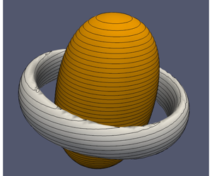
Figure 2. Isosurfaces of the initial PVA distribution  $\widetilde{\unicode[STIX]{x1D71B}}(\boldsymbol{x},t_{0})$ for modal amplitudes $\hat{\unicode[STIX]{x1D71B}}_{0}=1/4$, $\hat{\unicode[STIX]{x1D71B}}_{2,1}=1/8$, with (a) $\hat{\unicode[STIX]{x1D71B}}_{2,0}=-1/8$, isosurfaces $\widetilde{\unicode[STIX]{x1D71B}}=-0.01$ (grey) and $\widetilde{\unicode[STIX]{x1D71B}}=0.05$ (dark orange) and (b) $\hat{\unicode[STIX]{x1D71B}}_{2,0}=1/8$, isosurfaces $\widetilde{\unicode[STIX]{x1D71B}}=-0.015$ (grey) and $\widetilde{\unicode[STIX]{x1D71B}}=0.04$ (dark orange).
Numerical simulations with a relatively low resolution ( $128^{3}$ and $256^{3}$ grid points) showed that the vortex configuration is stable and displays a precessing PVA field. Only two particular cases are described here, in which the perturbation amplitudes $|\hat{\unicode[STIX]{x1D71B}}_{2,0}|=|\hat{\unicode[STIX]{x1D71B}}_{2,1}|=|\hat{\unicode[STIX]{x1D71B}}_{0}|/2$ are relatively large, in order to shown more clearly the vortex precession and that, even in these cases, the vortex remains stable. The initial PVA distributions are shown in figure 2 and their time evolution in movies 1, 2 and 3 (supplementary material available at https://doi.org/10.1017/jfm.2020.130). The precessing vortex may be conceptually regarded as a family of horizontal, two-dimensional Chaplygin–Lamb dipoles, parameterized by the depth $z$, whose trajectories are horizontal circles of radius proportional to the depth $z$ and centred along the vertical axis $\boldsymbol{e}_{z}$. The initial points of these Chaplygin–Lamb dipole trajectories are located along a straight vertically tilted axis, which corresponds to the vortex precession axis.
When the modal PVA amplitudes  $\hat{\unicode[STIX]{x1D71B}}_{0}$ and $\hat{\unicode[STIX]{x1D71B}}_{2,0}$ have different sign (initial PVA in figure 2(a) and time evolution in movies 1 and 2) this family of Chaplygin–Lamb dipoles is visualized from the two tilted spherical caps of PVA anomaly, with sign opposite to that of the vortex core, located above and below the vortex core. In this particular simulation the precessing vortex experienced $n_{p}=11$ anticlockwise precessions in a time period $\unicode[STIX]{x0394}t\simeq 4860$, which corresponds to an angular velocity $\unicode[STIX]{x1D714}_{0}=2\unicode[STIX]{x03C0}n_{p}/\unicode[STIX]{x0394}t\simeq 0.0142$.
When the zonal modal PVA amplitudes  $\hat{\unicode[STIX]{x1D71B}}_{0}$ and $\hat{\unicode[STIX]{x1D71B}}_{2,0}$ have the same sign (initial PVA in figure 2(b) and time evolution in movie 3) the family of Chaplygin–Lamb dipoles is easily inferred from the tilted torus of PVA anomaly, with sign opposite to that of the vortex core, located around the vortex core at mid-depth $z\simeq 0$. In this particular simulation the precessing vortex experienced $n_{p}=10$ anticlockwise precessions in a time period $\unicode[STIX]{x0394}t\simeq 4950$, which corresponds to an angular velocity $\unicode[STIX]{x1D714}_{0}=2\unicode[STIX]{x03C0}n_{p}/\unicode[STIX]{x0394}t\simeq 0.0127$. We note that, in the two cases described above, the PVA distributions of opposite sign to that of the vortex core, having a geometry similar to two spherical caps and one tilted torus, though of small amplitude in comparison with that of the vortex core, are necessary to maintain the vortex precession.
We conclude this section by asserting that the precession of a baroclinic vortex may be interpreted as the horizontal and circular advection by a large-amplitude spherical mode  $\unicode[STIX]{x1D71B}_{0}(\unicode[STIX]{x1D70C})$ of the small-amplitude vertical mode $\unicode[STIX]{x1D71B}_{2,0}(\unicode[STIX]{x1D70C},\unicode[STIX]{x1D703})$ tilted by a small-amplitude mode $\unicode[STIX]{x1D71B}_{2,1}(\unicode[STIX]{x1D70C},\unicode[STIX]{x1D703},\unicode[STIX]{x1D711})$. The next section provides the mathematical justification of this assertion.
4 Precessing vortex solutions
4.1 Steady-state solutions
Here we provide the steady-state solutions, in terms of the geopotential function  $\unicode[STIX]{x1D719}(\boldsymbol{x})$, as an intermediate step towards the time-dependent solution $\widetilde{\unicode[STIX]{x1D719}}(\boldsymbol{x},t)$. Since the modes $\text{j}_{l}(\unicode[STIX]{x1D70C})\,\text{Y}_{l}^{m}(\unicode[STIX]{x1D703},\unicode[STIX]{x1D711})$ are eigenfunctions of the Laplacian operator, the interior (superscript $i$) geopotentials are
 $$\begin{eqnarray}\displaystyle & \unicode[STIX]{x1D719}_{0}^{i}(\unicode[STIX]{x1D70C})\equiv {\hat{c}}_{0}\text{j}_{0}(\unicode[STIX]{x1D70C})\text{Y}_{0}^{0}=\hat{\unicode[STIX]{x1D719}}_{0}\text{j}_{0}(\unicode[STIX]{x1D70C}), & \displaystyle\end{eqnarray}$$
 $$\begin{eqnarray}\displaystyle & \unicode[STIX]{x1D719}_{2,0}^{i}(\unicode[STIX]{x1D70C},\unicode[STIX]{x1D703})\equiv {\hat{c}}_{2,0}\text{j}_{2}(\unicode[STIX]{x1D70C})\text{Y}_{2}^{0}(\unicode[STIX]{x1D703})=\hat{\unicode[STIX]{x1D719}}_{2,0}\text{j}_{2}(\unicode[STIX]{x1D70C})(3\cos ^{2}\unicode[STIX]{x1D703}-1), & \displaystyle\end{eqnarray}$$
 $$\begin{eqnarray}\displaystyle & \unicode[STIX]{x1D719}_{2,1}^{i}(\unicode[STIX]{x1D70C},\unicode[STIX]{x1D703},\unicode[STIX]{x1D711})\equiv {\hat{c}}_{2,1}\text{j}_{2}(\unicode[STIX]{x1D70C})\text{Y}_{2}^{1}(\unicode[STIX]{x1D703},\unicode[STIX]{x1D711})=\hat{\unicode[STIX]{x1D719}}_{2,1}\text{j}_{2}(\unicode[STIX]{x1D70C})\sin \unicode[STIX]{x1D703}\cos \unicode[STIX]{x1D703}\cos \unicode[STIX]{x1D711}, & \displaystyle\end{eqnarray}$$
 where  $\{\hat{\unicode[STIX]{x1D719}}_{0},\hat{\unicode[STIX]{x1D719}}_{2,0},\hat{\unicode[STIX]{x1D719}}_{2,1}\}=-\{\hat{\unicode[STIX]{x1D71B}}_{0},\hat{\unicode[STIX]{x1D71B}}_{2,0},\hat{\unicode[STIX]{x1D71B}}_{2,1}\}$ are real-valued geopotential modal amplitudes. The steady modal geopotentials are piecewise functions comprising the interior and exterior solutions, and are given by
 $$\begin{eqnarray}\displaystyle & \displaystyle {\displaystyle \frac{\unicode[STIX]{x1D719}_{0}(\unicode[STIX]{x1D70C})}{\hat{\unicode[STIX]{x1D719}}_{0}}}=\left\{\begin{array}{@{}ll@{}}\text{j}_{0}(\unicode[STIX]{x1D70C}),\quad & \unicode[STIX]{x1D70C}\leqslant \unicode[STIX]{x1D70C}_{1}\\ \text{j}_{0}(\unicode[STIX]{x1D70C}_{1})\left(1-{\displaystyle \frac{(\unicode[STIX]{x1D70C}_{1}-\unicode[STIX]{x1D70C})^{2}(2\unicode[STIX]{x1D70C}_{1}+\unicode[STIX]{x1D70C})}{6\unicode[STIX]{x1D70C}}}\right),\quad & \unicode[STIX]{x1D70C}_{1}<\unicode[STIX]{x1D70C},\end{array}\right. & \displaystyle\end{eqnarray}$$
 $$\begin{eqnarray}\displaystyle & \displaystyle {\displaystyle \frac{\unicode[STIX]{x1D719}_{2,0}(\unicode[STIX]{x1D70C},\unicode[STIX]{x1D703})}{\hat{\unicode[STIX]{x1D719}}_{2,0}(3\cos ^{2}\unicode[STIX]{x1D703}-1)}}={\displaystyle \frac{\unicode[STIX]{x1D719}_{2,1}(\unicode[STIX]{x1D70C},\unicode[STIX]{x1D703},\unicode[STIX]{x1D711})}{\hat{\unicode[STIX]{x1D719}}_{2,1}\sin \unicode[STIX]{x1D703}\cos \unicode[STIX]{x1D703}\cos \unicode[STIX]{x1D711}}}=\left\{\begin{array}{@{}ll@{}}\text{j}_{2}(\unicode[STIX]{x1D70C}),\quad & \unicode[STIX]{x1D70C}\leqslant \unicode[STIX]{x1D70C}_{2}\\ {\displaystyle \frac{\text{j}_{0}(\unicode[STIX]{x1D70C}_{2})}{15}}{\displaystyle \frac{\unicode[STIX]{x1D70C}^{5}-\unicode[STIX]{x1D70C}_{2}^{5}}{\unicode[STIX]{x1D70C}^{3}}},\quad & \unicode[STIX]{x1D70C}_{2}<\unicode[STIX]{x1D70C}.\end{array}\right. & \displaystyle\end{eqnarray}$$
 Finally, the steady geopotential  $\unicode[STIX]{x1D719}(\boldsymbol{x})$ is the sum of the three modes,
 $$\begin{eqnarray}\unicode[STIX]{x1D719}(\unicode[STIX]{x1D70C},\unicode[STIX]{x1D703},\unicode[STIX]{x1D711})\equiv \unicode[STIX]{x1D719}_{0}(\unicode[STIX]{x1D70C})+\unicode[STIX]{x1D719}_{2,0}(\unicode[STIX]{x1D70C},\unicode[STIX]{x1D703})+\unicode[STIX]{x1D719}_{2,1}(\unicode[STIX]{x1D70C},\unicode[STIX]{x1D703},\unicode[STIX]{x1D711}).\end{eqnarray}$$
 The interior and exterior solutions satisfy continuity at the internal radial boundaries  $\unicode[STIX]{x1D719}_{0}(\unicode[STIX]{x1D70C}_{1})=\text{j}_{0}(\unicode[STIX]{x1D70C}_{1})$ and $\unicode[STIX]{x1D719}_{2,0}(\unicode[STIX]{x1D70C}_{2},\unicode[STIX]{x1D703})=\unicode[STIX]{x1D719}_{2,1}(\unicode[STIX]{x1D70C}_{2},\unicode[STIX]{x1D703},\unicode[STIX]{x1D711})=0$, as well as continuity of the first and second radial derivatives,
 $$\begin{eqnarray}\left.\begin{array}{@{}c@{}}{\displaystyle \frac{\unicode[STIX]{x2202}\unicode[STIX]{x1D719}_{0}}{\unicode[STIX]{x2202}\unicode[STIX]{x1D70C}}}(\unicode[STIX]{x1D70C}_{1})=0,\quad {\displaystyle \frac{\unicode[STIX]{x2202}^{2}\unicode[STIX]{x1D719}_{0}}{\unicode[STIX]{x2202}\unicode[STIX]{x1D70C}^{2}}}(\unicode[STIX]{x1D70C}_{1})=-\hat{\unicode[STIX]{x1D719}}_{0}\text{j}_{0}(\unicode[STIX]{x1D70C}_{1}),\\ {\displaystyle \frac{1}{\unicode[STIX]{x1D70C}_{2}}}{\displaystyle \frac{\unicode[STIX]{x2202}\unicode[STIX]{x1D719}_{2,0}}{\unicode[STIX]{x2202}\unicode[STIX]{x1D70C}}}(\unicode[STIX]{x1D70C}_{2},\unicode[STIX]{x1D703})=-{\displaystyle \frac{1}{2}}{\displaystyle \frac{\unicode[STIX]{x2202}^{2}\unicode[STIX]{x1D719}_{2,0}}{\unicode[STIX]{x2202}\unicode[STIX]{x1D70C}^{2}}}(\unicode[STIX]{x1D70C}_{2},\unicode[STIX]{x1D703})=\hat{\unicode[STIX]{x1D719}}_{2,0}{\displaystyle \frac{\text{j}_{0}(\unicode[STIX]{x1D70C}_{2})}{3}}(3\cos ^{2}\unicode[STIX]{x1D703}-1),\\ {\displaystyle \frac{1}{\unicode[STIX]{x1D70C}_{2}}}{\displaystyle \frac{\unicode[STIX]{x2202}\unicode[STIX]{x1D719}_{2,1}}{\unicode[STIX]{x2202}\unicode[STIX]{x1D70C}}}(\unicode[STIX]{x1D70C}_{2},\unicode[STIX]{x1D703},\unicode[STIX]{x1D711})=-{\displaystyle \frac{1}{2}}{\displaystyle \frac{\unicode[STIX]{x2202}^{2}\unicode[STIX]{x1D719}_{2,1}}{\unicode[STIX]{x2202}\unicode[STIX]{x1D70C}^{2}}}(\unicode[STIX]{x1D70C}_{2},\unicode[STIX]{x1D703},\unicode[STIX]{x1D711})=\hat{\unicode[STIX]{x1D719}}_{2,1}{\displaystyle \frac{\text{j}_{0}(\unicode[STIX]{x1D70C}_{2})}{3}}\sin \unicode[STIX]{x1D703}\cos \unicode[STIX]{x1D703}\cos \unicode[STIX]{x1D719},\end{array}\right\}\end{eqnarray}$$
which ensures horizontal velocity, vertical stratification, vorticity and PVA continuity. For later reference we show, in spherical coordinates, the cylindrical velocity components of the three modes,
 $$\begin{eqnarray}\left.\begin{array}{@{}c@{}}{\displaystyle \frac{\boldsymbol{u}_{0}(\unicode[STIX]{x1D70C},\unicode[STIX]{x1D703})}{\hat{\unicode[STIX]{x1D719}}_{0}\sin \unicode[STIX]{x1D703}}}=-\boldsymbol{e}_{\unicode[STIX]{x1D711}}\left\{\begin{array}{@{}ll@{}}\text{j}_{1}(\unicode[STIX]{x1D70C}),\quad & \unicode[STIX]{x1D70C}\leqslant \unicode[STIX]{x1D70C}_{1}\\ {\displaystyle \frac{\text{j}_{0}(\unicode[STIX]{x1D70C}_{1})}{3}}{\displaystyle \frac{\unicode[STIX]{x1D70C}^{3}-\unicode[STIX]{x1D70C}_{1}^{3}}{\unicode[STIX]{x1D70C}^{2}}},\quad & \unicode[STIX]{x1D70C}_{1}<\unicode[STIX]{x1D70C},\end{array}\right.\\ {\displaystyle \frac{\boldsymbol{u}_{2,0}(\unicode[STIX]{x1D70C},\unicode[STIX]{x1D703})}{\hat{\unicode[STIX]{x1D719}}_{2,0}\sin \unicode[STIX]{x1D703}}}=\boldsymbol{e}_{\unicode[STIX]{x1D711}}\left\{\begin{array}{@{}ll@{}}\text{j}_{1}(\unicode[STIX]{x1D70C})(3\cos ^{2}\unicode[STIX]{x1D703}-1)-{\displaystyle \frac{\text{j}_{2}(\unicode[STIX]{x1D70C})}{\unicode[STIX]{x1D70C}}}3(5\cos ^{2}\unicode[STIX]{x1D703}-1),\quad & \unicode[STIX]{x1D70C}\leqslant \unicode[STIX]{x1D70C}_{2}\\ {\displaystyle \frac{\text{j}_{0}(\unicode[STIX]{x1D70C}_{2})}{15\unicode[STIX]{x1D70C}^{4}}}[(3(5\cos ^{2}\unicode[STIX]{x1D703}-1))\unicode[STIX]{x1D70C}_{2}^{5}-2\unicode[STIX]{x1D70C}^{5}],\quad & \unicode[STIX]{x1D70C}_{2}<\unicode[STIX]{x1D70C},\end{array}\right.\\ {\displaystyle \frac{\boldsymbol{u}_{2,1}(\unicode[STIX]{x1D70C},\unicode[STIX]{x1D703},\unicode[STIX]{x1D711})}{\hat{\unicode[STIX]{x1D719}}_{2,1}\cos \unicode[STIX]{x1D703}}}=\left\{\begin{array}{@{}l@{}}{\displaystyle \frac{\text{j}_{2}(\unicode[STIX]{x1D70C})}{2}}\sin \unicode[STIX]{x1D711}\boldsymbol{e}_{r}+\left(\sin ^{2}\unicode[STIX]{x1D703}\text{j}_{1}(\unicode[STIX]{x1D70C})+(5\cos ^{2}\unicode[STIX]{x1D703}-4){\displaystyle \frac{\text{j}_{2}(\unicode[STIX]{x1D70C})}{\unicode[STIX]{x1D70C}}}\right)\cos \unicode[STIX]{x1D711}\boldsymbol{e}_{\unicode[STIX]{x1D711}},\quad \\ \quad \unicode[STIX]{x1D70C}\leqslant \unicode[STIX]{x1D70C}_{2}\quad \\ {\displaystyle \frac{\text{j}_{0}(\unicode[STIX]{x1D70C}_{2})}{15\unicode[STIX]{x1D70C}^{4}}}[(\unicode[STIX]{x1D70C}^{5}-\unicode[STIX]{x1D70C}_{2}^{5})\sin \unicode[STIX]{x1D711}\boldsymbol{e}_{r}+(\unicode[STIX]{x1D70C}^{5}-\unicode[STIX]{x1D70C}_{2}^{5}(5\cos ^{2}\unicode[STIX]{x1D703}-4))\cos \unicode[STIX]{x1D711}\boldsymbol{e}_{\unicode[STIX]{x1D711}}],\quad \\ \quad \unicode[STIX]{x1D70C}_{2}<\unicode[STIX]{x1D70C}.\quad \end{array}\right.\end{array}\right\}\end{eqnarray}$$
For later use we also provide the vertical vorticity of the spherical mode,
 $$\begin{eqnarray}{\displaystyle \frac{\unicode[STIX]{x1D701}_{0}(\unicode[STIX]{x1D70C},\unicode[STIX]{x1D703})}{\hat{\unicode[STIX]{x1D719}}_{0}}}=\left\{\begin{array}{@{}ll@{}}-2{\displaystyle \frac{\text{j}_{1}(\unicode[STIX]{x1D70C})}{\unicode[STIX]{x1D70C}}}+\text{j}_{2}(\unicode[STIX]{x1D70C})\sin ^{2}\unicode[STIX]{x1D703},\quad & \unicode[STIX]{x1D70C}\leqslant \unicode[STIX]{x1D70C}_{1}\\ {\displaystyle \frac{\text{j}_{0}(\unicode[STIX]{x1D70C}_{1})}{3}}\left[(3\cos ^{2}\unicode[STIX]{x1D703}-1){\displaystyle \frac{\unicode[STIX]{x1D70C}_{2}^{3}}{\unicode[STIX]{x1D70C}^{3}}}-2\right],\quad & \unicode[STIX]{x1D70C}_{1}<\unicode[STIX]{x1D70C},\end{array}\right.\end{eqnarray}$$
 as well as the exterior vertical vorticity of modes  $\{2,0\}$ and $\{2,1\}$,
 $$\begin{eqnarray}\left.\begin{array}{@{}c@{}}\unicode[STIX]{x1D701}_{2,0}^{e}(\unicode[STIX]{x1D70C},\unicode[STIX]{x1D703})=\hat{\unicode[STIX]{x1D719}}_{2,0}\text{j}_{0}(\unicode[STIX]{x1D70C}_{2}){\displaystyle \frac{15\unicode[STIX]{x1D70C}_{2}^{5}(4\cos (2\unicode[STIX]{x1D703})+7\cos (4\unicode[STIX]{x1D703}))-32\unicode[STIX]{x1D70C}^{5}+27\unicode[STIX]{x1D70C}_{2}^{5}}{120\unicode[STIX]{x1D70C}^{5}}},\\ \unicode[STIX]{x1D701}_{2,1}^{e}(\unicode[STIX]{x1D70C},\unicode[STIX]{x1D703},\unicode[STIX]{x1D711})=\hat{\unicode[STIX]{x1D719}}_{2,1}\text{j}_{0}(\unicode[STIX]{x1D70C}_{2}),\unicode[STIX]{x1D70C}_{2}^{5}{\displaystyle \frac{\sin (2\unicode[STIX]{x1D703})(7\cos (2\unicode[STIX]{x1D703})+1)\cos \unicode[STIX]{x1D711}}{12\unicode[STIX]{x1D70C}^{5}}},\end{array}\right\}\end{eqnarray}$$
 and we note that, since these two modes have zero exterior PVA, their exterior vertical vorticity equals, with opposite sign, their exterior vertical stratification (that is,  $\unicode[STIX]{x1D701}_{2,0}^{e}(\unicode[STIX]{x1D70C},\unicode[STIX]{x1D703})=-{\mathcal{S}}_{2,0}^{e}(\unicode[STIX]{x1D70C},\unicode[STIX]{x1D703})$ and $\unicode[STIX]{x1D701}_{2,1}^{e}(\unicode[STIX]{x1D70C},\unicode[STIX]{x1D703},\unicode[STIX]{x1D711})=-{\mathcal{S}}_{2,0}^{e}(\unicode[STIX]{x1D70C},\unicode[STIX]{x1D703},\unicode[STIX]{x1D711})$).
4.2 The far field of the steady solutions
The solutions in the previous subsection in terms of the geopotential  $\unicode[STIX]{x1D719}(\boldsymbol{x})$ are steady-state solutions, but are not completely satisfactory, in the sense that the velocity and density stratification anomaly fields do not vanish as $\unicode[STIX]{x1D70C}\rightarrow \infty$. For example, from (4.9), the far-field velocity of the spherical mode,
 $$\begin{eqnarray}\boldsymbol{u}_{0}(\unicode[STIX]{x1D70C},\unicode[STIX]{x1D703})\sim {\displaystyle \frac{\hat{\unicode[STIX]{x1D71B}}_{0}}{3}}\text{j}_{0}(\unicode[STIX]{x1D70C}_{1})\unicode[STIX]{x1D70C}\sin \unicode[STIX]{x1D703}\boldsymbol{e}_{\unicode[STIX]{x1D711}}={\displaystyle \frac{\hat{\unicode[STIX]{x1D71B}}_{0}}{3}}\text{j}_{0}(\unicode[STIX]{x1D70C}_{1})r(\unicode[STIX]{x1D70C},\unicode[STIX]{x1D703})\boldsymbol{e}_{\unicode[STIX]{x1D711}}\equiv \boldsymbol{u}_{0}^{\infty }(r),\end{eqnarray}$$
 increases as  $r$, and therefore tends to a constant vertical vorticity
 $$\begin{eqnarray}\unicode[STIX]{x1D73B}_{0}^{\infty }\equiv \unicode[STIX]{x1D735}\times \boldsymbol{u}_{0}^{\infty }={\textstyle \frac{2}{3}}\hat{\unicode[STIX]{x1D71B}}_{0}\text{j}_{0}(\unicode[STIX]{x1D70C}_{1})\boldsymbol{e}_{z}\equiv \unicode[STIX]{x1D701}_{0}^{\infty }\boldsymbol{e}_{z}.\end{eqnarray}$$
 The far-field velocity of the mode  $\{2,0\}$, from (4.9),
 $$\begin{eqnarray}\boldsymbol{u}_{2,0}(\unicode[STIX]{x1D70C},\unicode[STIX]{x1D703})\sim {\textstyle \frac{2}{15}}\hat{\unicode[STIX]{x1D71B}}_{2,0}\text{j}_{0}(\unicode[STIX]{x1D70C}_{2})\unicode[STIX]{x1D70C}\sin \unicode[STIX]{x1D703}\boldsymbol{e}_{\unicode[STIX]{x1D711}}={\textstyle \frac{2}{15}}\hat{\unicode[STIX]{x1D71B}}_{2,0}\text{j}_{0}(\unicode[STIX]{x1D70C}_{2})r(\unicode[STIX]{x1D70C},\unicode[STIX]{x1D703})\boldsymbol{e}_{\unicode[STIX]{x1D711}}\equiv \boldsymbol{u}_{2,0}^{\infty }(r),\end{eqnarray}$$
 increases also as  $r$, and also tends to a constant far-field vertical vorticity
 $$\begin{eqnarray}\unicode[STIX]{x1D73B}_{2,0}^{\infty }\equiv \unicode[STIX]{x1D735}\times \boldsymbol{u}_{2,0}^{\infty }={\textstyle \frac{4}{15}}\hat{\unicode[STIX]{x1D71B}}_{2,0}\text{j}_{0}(\unicode[STIX]{x1D70C}_{2})\boldsymbol{e}_{z}\equiv \unicode[STIX]{x1D701}_{2,0}^{\infty }\boldsymbol{e}_{z},\end{eqnarray}$$
 while the far-field velocity of mode  $\{2,1\}$
 $$\begin{eqnarray}\boldsymbol{u}_{2,1}(\unicode[STIX]{x1D70C},\unicode[STIX]{x1D703})\sim {\displaystyle \frac{\hat{\unicode[STIX]{x1D71B}}_{2,1}}{15}}\text{j}_{0}(\unicode[STIX]{x1D70C}_{2})\unicode[STIX]{x1D70C}\cos \unicode[STIX]{x1D703}(\sin \unicode[STIX]{x1D711}\boldsymbol{e}_{r}+\cos \unicode[STIX]{x1D711}\boldsymbol{e}_{\unicode[STIX]{x1D711}})={\displaystyle \frac{\hat{\unicode[STIX]{x1D71B}}_{2,1}}{15}}\text{j}_{0}(\unicode[STIX]{x1D70C}_{2})z\boldsymbol{e}_{y}\equiv \boldsymbol{u}_{2,1}^{\infty },(z)\end{eqnarray}$$
 increases as  $z$ and therefore tends to a constant far-field horizontal vorticity
 $$\begin{eqnarray}\unicode[STIX]{x1D73B}_{2,1}^{\infty }\equiv \unicode[STIX]{x1D735}\times \boldsymbol{u}_{2,1}^{\infty }=-\hat{\unicode[STIX]{x1D71B}}_{2,1}{\displaystyle \frac{\text{j}_{0}(\unicode[STIX]{x1D70C}_{2})}{15}}\boldsymbol{e}_{x}\equiv \unicode[STIX]{x1D709}_{2,1}^{\infty }\boldsymbol{e}_{x}.\end{eqnarray}$$
 Since modes  $\{2,0\}$ and $\{2,1\}$ have zero exterior PVA, their far-field vertical vorticity equals the (negative of the) far-field density stratification, which implies, from (4.10), that
 $$\begin{eqnarray}\displaystyle & \displaystyle \unicode[STIX]{x1D701}_{2,0}^{\infty }\equiv \lim _{\unicode[STIX]{x1D70C}\rightarrow \infty }\unicode[STIX]{x1D701}_{2,0}^{e}(\unicode[STIX]{x1D70C},\unicode[STIX]{x1D703})=-{\mathcal{S}}_{2,0}^{\infty }\equiv -\lim _{\unicode[STIX]{x1D70C}\rightarrow \infty }{\mathcal{S}}_{2,0}^{e}(\unicode[STIX]{x1D70C},\unicode[STIX]{x1D703})={\textstyle \frac{4}{15}}\hat{\unicode[STIX]{x1D71B}}_{2,0}\text{j}_{0}(\unicode[STIX]{x1D70C}_{2}), & \displaystyle\end{eqnarray}$$
 $$\begin{eqnarray}\displaystyle & \displaystyle \unicode[STIX]{x1D701}_{2,1}^{\infty }\equiv \lim _{\unicode[STIX]{x1D70C}\rightarrow \infty }\unicode[STIX]{x1D701}_{2,1}^{e}(\unicode[STIX]{x1D70C},\unicode[STIX]{x1D703},\unicode[STIX]{x1D711})=-{\mathcal{S}}_{2,1}^{\infty }\equiv -\lim _{\unicode[STIX]{x1D70C}\rightarrow \infty }{\mathcal{S}}_{2,1}^{e}(\unicode[STIX]{x1D70C},\unicode[STIX]{x1D703},\unicode[STIX]{x1D711})=0, & \displaystyle\end{eqnarray}$$
 so that mode  $\{2,0\}$ induces also a constant far-field density stratification ${\mathcal{S}}_{2,0}^{\infty }$.
4.3 Unsteady approximate solutions with vanishing far fields
In order to remove the finite far fields from the steady modal geopotentials, three background modal geopotentials,  $\bar{\unicode[STIX]{x1D719}}_{0}(\unicode[STIX]{x1D70C})$, $\bar{\unicode[STIX]{x1D719}}_{2,0}(\unicode[STIX]{x1D70C},\unicode[STIX]{x1D703})$ and $\bar{\unicode[STIX]{x1D719}}_{2,1}(\unicode[STIX]{x1D70C},\unicode[STIX]{x1D703},\unicode[STIX]{x1D711})$, are added to the full domain of the steady-state solution $\unicode[STIX]{x1D719}(\boldsymbol{x})$. These background modal geopotentials are, with opposite sign, the leading terms as $\unicode[STIX]{x1D70C}\rightarrow \infty$ of the steady-state modal geopotentials given by (4.5): that is,
 $$\begin{eqnarray}\displaystyle & \displaystyle {\displaystyle \frac{\bar{\unicode[STIX]{x1D719}}_{0}(\unicode[STIX]{x1D70C})}{\hat{\unicode[STIX]{x1D71B}}_{0}}}=-{\displaystyle \frac{\text{j}_{0}(\unicode[STIX]{x1D70C}_{1})}{6}}\unicode[STIX]{x1D70C}^{2}, & \displaystyle\end{eqnarray}$$
 $$\begin{eqnarray}\displaystyle & \displaystyle {\displaystyle \frac{\bar{\unicode[STIX]{x1D719}}_{2,0}(\unicode[STIX]{x1D70C},\unicode[STIX]{x1D703})}{\hat{\unicode[STIX]{x1D71B}}_{2,0}(3\cos ^{2}\unicode[STIX]{x1D703}-1)}}={\displaystyle \frac{\bar{\unicode[STIX]{x1D719}}_{2,1}(\unicode[STIX]{x1D70C},\unicode[STIX]{x1D703},\unicode[STIX]{x1D711})}{\hat{\unicode[STIX]{x1D71B}}_{2,1}\sin \unicode[STIX]{x1D703}\cos \unicode[STIX]{x1D703}\cos \unicode[STIX]{x1D711}}}={\displaystyle \frac{\text{j}_{0}(\unicode[STIX]{x1D70C}_{2})}{15}}\unicode[STIX]{x1D70C}^{2}, & \displaystyle\end{eqnarray}$$
 so that the background geopotential  $\bar{\unicode[STIX]{x1D719}}(\boldsymbol{x})$ is the sum of the three contributions,
 $$\begin{eqnarray}\bar{\unicode[STIX]{x1D719}}(\unicode[STIX]{x1D70C},\unicode[STIX]{x1D703},\unicode[STIX]{x1D711})=\bar{\unicode[STIX]{x1D719}}_{0}(\unicode[STIX]{x1D70C})+\bar{\unicode[STIX]{x1D719}}_{2,0}(\unicode[STIX]{x1D70C},\unicode[STIX]{x1D703})+\bar{\unicode[STIX]{x1D719}}_{2,1}(\unicode[STIX]{x1D70C},\unicode[STIX]{x1D703},\unicode[STIX]{x1D711}).\end{eqnarray}$$
 Addition of the background geopotential  $\bar{\unicode[STIX]{x1D719}}(\boldsymbol{x})$ to the vortex assures vanishing fields at infinity, but at the expense of making the vortex unsteady, so that we can only define the initial condition $\widetilde{\unicode[STIX]{x1D719}}(\boldsymbol{x},t_{0})$ of the unsteady geopotential $\widetilde{\unicode[STIX]{x1D719}}(\boldsymbol{x},t)$ as
 $$\begin{eqnarray}\widetilde{\unicode[STIX]{x1D719}}(\boldsymbol{x},t_{0})=\unicode[STIX]{x1D719}(\boldsymbol{x})+\bar{\unicode[STIX]{x1D719}}(\boldsymbol{x}).\end{eqnarray}$$
 Since  $\unicode[STIX]{x1D6FB}^{2}\bar{\unicode[STIX]{x1D719}}_{0}=-\hat{\unicode[STIX]{x1D71B}}_{0}\text{j}_{0}(\unicode[STIX]{x1D70C}_{1})$ and $\unicode[STIX]{x1D6FB}^{2}\bar{\unicode[STIX]{x1D719}}_{2,0}=\unicode[STIX]{x1D6FB}^{2}\bar{\unicode[STIX]{x1D719}}_{2,1}=0$, the PVA of the initial geopotential condition (4.22) is exactly $\widetilde{\unicode[STIX]{x1D71B}}(\unicode[STIX]{x1D70C},\unicode[STIX]{x1D703},\unicode[STIX]{x1D711},t_{0})$, as given by (3.4).
The background flow  $\bar{\boldsymbol{u}}(\boldsymbol{x})\equiv -\unicode[STIX]{x1D735}\times (\bar{\unicode[STIX]{x1D719}}(\boldsymbol{x})\,\boldsymbol{e}_{z})$ is horizontal and is the sum of the background modal velocity fields
 $$\begin{eqnarray}\left.\begin{array}{@{}c@{}}\bar{\boldsymbol{u}}_{0}(r)=-\boldsymbol{u}_{0}^{\infty }(r)=-\hat{\unicode[STIX]{x1D71B}}_{0}{\displaystyle \frac{\text{j}_{0}(\unicode[STIX]{x1D70C}_{1})}{3}}r\boldsymbol{e}_{\unicode[STIX]{x1D711}},\\ \bar{\boldsymbol{u}}_{2,0}(r)=-\boldsymbol{u}_{2,0}^{\infty }(r)=-\hat{\unicode[STIX]{x1D71B}}_{2,0}{\displaystyle \frac{2\text{j}_{0}(\unicode[STIX]{x1D70C}_{2})}{15}}r\boldsymbol{e}_{\unicode[STIX]{x1D711}},\\ \bar{\boldsymbol{u}}_{2,1}(z)=-\boldsymbol{u}_{2,1}^{\infty }(z)=-\hat{\unicode[STIX]{x1D71B}}_{2,1}{\displaystyle \frac{\text{j}_{0}(\unicode[STIX]{x1D70C}_{2})}{15}}z\boldsymbol{e}_{y}.\end{array}\right\}\end{eqnarray}$$
 The position  $\bar{\boldsymbol{r}}(\boldsymbol{X},t)$ of particles $\boldsymbol{X}=(X,Y,Z)$ moving with the background flow $\bar{\boldsymbol{u}}(\boldsymbol{x})=\bar{\boldsymbol{u}}_{0}(r)+\bar{\boldsymbol{u}}_{2,0}(r)+\bar{\boldsymbol{u}}_{2,1}(z)$ therefore satisfies the equation
 $$\begin{eqnarray}\displaystyle {\displaystyle \frac{\unicode[STIX]{x2202}\bar{\boldsymbol{r}}}{\unicode[STIX]{x2202}t}}(\boldsymbol{X},t) & = & \displaystyle \bar{\boldsymbol{u}}_{0}(\bar{r}(\boldsymbol{X},t))+\bar{\boldsymbol{u}}_{2,0}(\bar{r}(\boldsymbol{X},t))+\bar{\boldsymbol{u}}_{2,1}(\bar{z}(\boldsymbol{X},t))\nonumber\\ \displaystyle & = & \displaystyle \unicode[STIX]{x1D714}_{0}\boldsymbol{e}_{z}\times \bar{\boldsymbol{r}}(\boldsymbol{X},t)+\unicode[STIX]{x1D709}_{0}\boldsymbol{e}_{z}\boldsymbol{\cdot }\bar{\boldsymbol{r}}(\boldsymbol{X},t)\boldsymbol{e}_{y}\nonumber\\ \displaystyle & = & \displaystyle \unicode[STIX]{x1D714}_{0}(\bar{r}(\boldsymbol{X},t)\boldsymbol{e}_{\unicode[STIX]{x1D711}}+\unicode[STIX]{x1D6FE}_{0}Z\boldsymbol{e}_{y}),\end{eqnarray}$$
 where, obviously,  $\bar{z}(\boldsymbol{X},t)=z=Z=\boldsymbol{e}_{z}\boldsymbol{\cdot }\bar{\boldsymbol{r}}(\boldsymbol{X},t)$, since $\bar{\boldsymbol{u}}(\boldsymbol{x})$ is horizontal, and we have defined the angular velocity $\unicode[STIX]{x1D714}_{0}$, vertical shearing $\unicode[STIX]{x1D709}_{0}$, and their ratio $\unicode[STIX]{x1D6FE}_{0}$ as
 $$\begin{eqnarray}\unicode[STIX]{x1D714}_{0}\equiv -\hat{\unicode[STIX]{x1D71B}}_{0}{\displaystyle \frac{\text{j}_{0}(\unicode[STIX]{x1D70C}_{1})}{3}}-\hat{\unicode[STIX]{x1D71B}}_{2,0}{\displaystyle \frac{2\text{j}_{0}(\unicode[STIX]{x1D70C}_{2})}{15}},\quad \unicode[STIX]{x1D709}_{0}\equiv -\hat{\unicode[STIX]{x1D71B}}_{2,1}{\displaystyle \frac{\text{j}_{0}(\unicode[STIX]{x1D70C}_{2})}{15}},\quad \unicode[STIX]{x1D6FE}_{0}\equiv {\displaystyle \frac{\unicode[STIX]{x1D709}_{0}}{\unicode[STIX]{x1D714}_{0}}},\end{eqnarray}$$
 assuming, in the definition of the ratio  $\unicode[STIX]{x1D6FE}_{0}$, that $\unicode[STIX]{x1D714}_{0}\neq 0$. The solution to (4.24) is
 $$\begin{eqnarray}\bar{\boldsymbol{r}}(\boldsymbol{X},t)+\unicode[STIX]{x1D6FE}_{0}Z\boldsymbol{e}_{x}=\unicode[STIX]{x1D64D}[\unicode[STIX]{x1D714}_{0}t]\boldsymbol{\cdot }(\boldsymbol{X}+\unicode[STIX]{x1D6FE}_{0}Z\boldsymbol{e}_{x}),\end{eqnarray}$$
 where  $\unicode[STIX]{x1D64D}[\unicode[STIX]{x1D6FC}]$ is the two-dimensional rotation tensor that rotates a vector $(x,y)$ counterclockwise through an angle $\unicode[STIX]{x1D6FC}$. The background motion is therefore a horizontal rotation of the particles $(X,Y,Z)$ by an angle $\unicode[STIX]{x1D714}_{0}t$ around the point $(-\unicode[STIX]{x1D6FE}_{0}Z,0,Z)$. The background motion is not a rigid motion in the three-dimensional space, due to the constant $\unicode[STIX]{x1D6FE}_{0}$, but it might be thought of as a continuous family, parameterized by the vertical coordinate $z$, of changes of reference of horizontal two-dimensional frames rotating around the points $(-\unicode[STIX]{x1D6FE}_{0}Z,0,Z)=(-\unicode[STIX]{x1D6FE}_{0},0,1)Z$, where $\unicode[STIX]{x1D6FE}_{0}$ defines the tangent of the axis comprising the centres of rotation at every depth $z$. More importantly, since the streamlines of the horizontal background flow are circles, the background flow has no diffluence, no bifurcation points, and therefore will not largely distort the modal distributions, as long as the vertical shear $\unicode[STIX]{x1D709}_{0}$ remains small or the ratio $|\unicode[STIX]{x1D6FE}_{0}|\ll 1$. This property is characteristic of modes $\text{j}_{l}(\unicode[STIX]{x1D70C})\text{Y}_{l}^{0,\pm 1}(\unicode[STIX]{x1D703},\unicode[STIX]{x1D711})$, where the azimuthal wavenumber is 0 or $\pm 1$.
The particles  $\boldsymbol{X}$ located at position $\boldsymbol{x}$ at time $t$ are therefore given by $\bar{\boldsymbol{R}}(\boldsymbol{x},t)$,
 $$\begin{eqnarray}\bar{\boldsymbol{R}}(\boldsymbol{x},t)+\unicode[STIX]{x1D6FE}_{0}z\boldsymbol{e}_{x}=\unicode[STIX]{x1D64D}^{\imath }[\unicode[STIX]{x1D714}_{0}t]\boldsymbol{\cdot }(\boldsymbol{x}+\unicode[STIX]{x1D6FE}_{0}z\boldsymbol{e}_{x}),\end{eqnarray}$$
 where  $\unicode[STIX]{x1D64D}^{\imath }[\unicode[STIX]{x1D6FC}]=\unicode[STIX]{x1D64D}[-\unicode[STIX]{x1D6FC}]$ is the tensor inverse of $\unicode[STIX]{x1D64D}[\unicode[STIX]{x1D6FC}]$. Explicitly, in Cartesian coordinates,
 $$\begin{eqnarray}\left.\begin{array}{@{}c@{}}\bar{X}(\boldsymbol{x},t)+\unicode[STIX]{x1D6FE}_{0}z=(x+\unicode[STIX]{x1D6FE}_{0}z)\cos (\unicode[STIX]{x1D714}_{0}t)+y\sin (\unicode[STIX]{x1D714}_{0}t),\\ \bar{Y}(\boldsymbol{x},t)=-(x+\unicode[STIX]{x1D6FE}_{0}z)\sin (\unicode[STIX]{x1D714}_{0}t)+y\cos (\unicode[STIX]{x1D714}_{0}t).\end{array}\right\}\end{eqnarray}$$
 Given the background flow  $\bar{\boldsymbol{u}}(\boldsymbol{x},t)$, we postulate that, for small ratios $\unicode[STIX]{x1D6FE}_{0}$, an approximate solution to $\widetilde{\unicode[STIX]{x1D71B}}(\boldsymbol{x},t)$ is the unsteady solution $\check{\unicode[STIX]{x1D71B}}(\boldsymbol{x},t)$, defined as the initial PVA distribution $\widetilde{\unicode[STIX]{x1D71B}}(\boldsymbol{x},t_{0})$ materially advected by the background flow – that is,
 $$\begin{eqnarray}\check{\unicode[STIX]{x1D71B}}(\boldsymbol{x},t)\equiv \widetilde{\unicode[STIX]{x1D71B}}(\bar{\boldsymbol{R}}(\boldsymbol{x},t),t_{0})\simeq \widetilde{\unicode[STIX]{x1D71B}}(\boldsymbol{x},t).\end{eqnarray}$$
 Clearly, since  $\bar{\boldsymbol{R}}(\boldsymbol{x},t_{0})=\boldsymbol{x}$ and $\widetilde{\boldsymbol{u}}\boldsymbol{\cdot }\unicode[STIX]{x1D735}\widetilde{\unicode[STIX]{x1D71B}}(\boldsymbol{x},t_{0})=\bar{\boldsymbol{u}}\boldsymbol{\cdot }\unicode[STIX]{x1D735}\widetilde{\unicode[STIX]{x1D71B}}(\boldsymbol{x},t_{0})$ (appendix A), we have
 $$\begin{eqnarray}\check{\unicode[STIX]{x1D71B}}(\boldsymbol{x},t_{0})=\widetilde{\unicode[STIX]{x1D71B}}(\boldsymbol{x},t_{0}),\quad {\displaystyle \frac{\unicode[STIX]{x2202}\check{\unicode[STIX]{x1D71B}}}{\unicode[STIX]{x2202}t}}(\boldsymbol{x},t_{0})={\displaystyle \frac{\unicode[STIX]{x2202}\widetilde{\unicode[STIX]{x1D71B}}}{\unicode[STIX]{x2202}t}}(\boldsymbol{x},t_{0}).\end{eqnarray}$$
 However, higher-order time derivatives at the initial time  $t_{0}$ do not coincide. An example of the approximate solution $\check{\unicode[STIX]{x1D71B}}(\boldsymbol{x},t)$ is shown in movie 4. The precession frequency $\unicode[STIX]{x1D714}_{0}$ of the approximate solution $\check{\unicode[STIX]{x1D71B}}(\boldsymbol{x},t)$, given by (4.25), predicts precession frequencies $\unicode[STIX]{x1D71B}_{0}\simeq 0.0167$ and $\unicode[STIX]{x1D71B}_{0}\simeq 0.0195$ for the modal PVA amplitudes $|\hat{\unicode[STIX]{x1D71B}}_{2,0}|=|\hat{\unicode[STIX]{x1D71B}}_{2,1}|=|\hat{\unicode[STIX]{x1D71B}}_{0}|/2$ of the numerical simulations described in the previous section, which, taking into account the large amplitudes considered, are reasonable approximations to the numerical values (0.0142 and 0.0127, respectively).
The corresponding geopotential  $\check{\unicode[STIX]{x1D719}}(\boldsymbol{x},t)$, consistent with relation (2.2), must satisfy $\unicode[STIX]{x1D6FB}^{2}\check{\unicode[STIX]{x1D719}}(\boldsymbol{x},t)=\check{\unicode[STIX]{x1D71B}}(\boldsymbol{x},t)$, with vanishing far-field conditions. Inverting $\unicode[STIX]{x1D6FB}^{2}\check{\unicode[STIX]{x1D719}}(\boldsymbol{x},t)=\check{\unicode[STIX]{x1D71B}}(\boldsymbol{x},t)\equiv \widetilde{\unicode[STIX]{x1D71B}}(\bar{\boldsymbol{R}}(\boldsymbol{x},t),t_{0})$ is not trivial since the three-dimensional Laplacian $\unicode[STIX]{x1D6FB}^{2}$ is not invariant under the transformation $\bar{\boldsymbol{R}}(\boldsymbol{x},t)$ for $\unicode[STIX]{x1D6FE}_{0}\neq 0$, and therefore $\check{\unicode[STIX]{x1D719}}(\boldsymbol{x},t)$ differs from $\check{\unicode[STIX]{x1D719}}(\bar{\boldsymbol{R}}(\boldsymbol{x},t),t_{0})=\widetilde{\unicode[STIX]{x1D719}}(\bar{\boldsymbol{R}}(\boldsymbol{x},t),t_{0})$ at $t>t_{0}$. On the other hand, the geopotential $\check{\unicode[STIX]{x1D719}}(\boldsymbol{x},t)$, symbolically defined as $\check{\unicode[STIX]{x1D719}}(\boldsymbol{x},t)=\unicode[STIX]{x1D6FB}^{-2}\check{\unicode[STIX]{x1D71B}}(\boldsymbol{x},t)$, is not an exact solution to the dynamical equation (2.3) at $t>t_{0}$ because (a) $\check{\unicode[STIX]{x1D71B}}(\boldsymbol{x},t)$ is only an approximation to $\widetilde{\unicode[STIX]{x1D71B}}(\boldsymbol{x},t)$, (b) $\widetilde{\unicode[STIX]{x1D719}}(\boldsymbol{x},t)$ is assumed to satisfy the dynamical equation, and (c) the initial conditions coincide (4.30).
5 Concluding remarks
In this work we have provided a simple mathematical model, based on three potential vorticity anomaly modes in spherical geometry, which explains, under the quasi-geostrophic approximation, the permanent precession of geophysical vortices. The precession of this new coherent vortex structure is interpreted as the horizontal and circular advection by the background flow associated with the spherical mode  $\hat{\unicode[STIX]{x1D71B}}_{0}\text{j}_{0}(\unicode[STIX]{x1D70C})$ of the mode $\hat{\unicode[STIX]{x1D71B}}_{2,0}\text{j}_{2}(\unicode[STIX]{x1D70C})\text{Y}_{2}^{0}(\unicode[STIX]{x1D70C},\unicode[STIX]{x1D703})$ vertically tilted by the mode $\hat{\unicode[STIX]{x1D71B}}_{2,1}\text{j}_{2}(\unicode[STIX]{x1D70C})\text{Y}_{2}^{1}(\unicode[STIX]{x1D70C},\unicode[STIX]{x1D703},\unicode[STIX]{x1D711})$. Unlike what happens in the case of the quasi-geostrophic spherical dipole, which is a periodic rigid motion composed of mode-0 $\text{j}_{0}(\unicode[STIX]{x1D70C})$ and modes $\text{j}_{1}(\unicode[STIX]{x1D70C})\text{Y}_{1}^{0,\pm 1}(\unicode[STIX]{x1D703},\unicode[STIX]{x1D711})$, the potential vorticity anomaly in the precessing vortex experiences a periodic motion that is not rigid, and therefore is not steady in any reference frame.
We may therefore associate with the spherical QG vortex, whose potential vorticity anomaly is given only by the mode-0  $\hat{\unicode[STIX]{x1D71B}}_{0}\text{j}_{0}(\unicode[STIX]{x1D70C})$, an intrinsic frequency $\unicode[STIX]{x1D714}_{0}=-\hat{\unicode[STIX]{x1D71B}}_{0}\text{j}_{0}(\unicode[STIX]{x1D70C}_{1})/3$. This intrinsic frequency only shows up when the vortex is perturbed in some specific ways. Perturbations of degree 1 correspond to the uniformly translating QG vortex dipole. If the vortex is perturbed with the zonal mode $\{1,0\}$ (that is, adding $\hat{\unicode[STIX]{x1D71B}}_{1,0}\text{j}_{1}(\unicode[STIX]{x1D70C})\text{Y}_{1}^{0}(\unicode[STIX]{x1D703})$), the vertical structure of the vortex changes but the symmetry around the vertical axis is preserved and the intrinsic frequency remains hidden. However, if the perturbation is the non-zonal mode $\{1,1\}$ (that is, $\hat{\unicode[STIX]{x1D71B}}_{1,\pm 1}\text{j}_{1}(\unicode[STIX]{x1D70C})\text{Y}_{1}^{\pm 1}(\unicode[STIX]{x1D703},\unicode[STIX]{x1D711})$), the intrinsic frequency is detectable since the vortex dipole acquires a circular trajectory of signed radius $\hat{\unicode[STIX]{x1D71B}}_{1,\pm 1}/\hat{\unicode[STIX]{x1D71B}}_{0}$ and frequency $\unicode[STIX]{x1D714}_{0}$. In the precessing vortex model presented here the vortex also has an intrinsic frequency, given in this case by the zonal modes $\unicode[STIX]{x1D714}_{0}=-\hat{\unicode[STIX]{x1D71B}}_{0}\text{j}_{0}(\unicode[STIX]{x1D70C}_{1})/3-2\hat{\unicode[STIX]{x1D71B}}_{2,0}\text{j}_{0}(\unicode[STIX]{x1D70C}_{2})/15$. If the vortex is perturbed with the non-zonal mode $\{2,1\}$ (that is, $\hat{\unicode[STIX]{x1D71B}}_{2,\pm 1}\text{j}_{2}(\unicode[STIX]{x1D70C})\text{Y}_{2}^{\pm 1}(\unicode[STIX]{x1D703},\unicode[STIX]{x1D711})$), the intrinsic vortex frequency becomes detectable in the periodic precession of the vortex vertical axis, which tilts with slope $\unicode[STIX]{x1D6FE}_{0}=(-\hat{\unicode[STIX]{x1D71B}}_{2,1}\text{j}_{0}(\unicode[STIX]{x1D70C}_{2})/15)/\unicode[STIX]{x1D714}_{0}$. In both cases, the dipole vortex and the precessing vortex, the vortices have an intrinsic frequency which shows up when the vortex is perturbed in a non-zonal azimuthal way.
The existence of the permanent tilting modes described here are relevant to our understanding of vertical alignment of geophysical vortices. We may think of any small-amplitude, but otherwise arbitrary PVA distribution as decomposed by a sum of PVA modes  $\hat{\unicode[STIX]{x1D71B}}_{l,m}\text{j}_{l}(\unicode[STIX]{x1D70C})\text{Y}_{l}^{m}(\unicode[STIX]{x1D703},\unicode[STIX]{x1D711})$. Many of these excited modes are evanescent in the sense that their PVA distributions evolve into highly sheared structures, mainly by spiralling around the vortex centre due to the advection by the large-amplitude vortex spherical mode, so that their radial wavenumber increases indefinitely and are ultimately dumped by diffusive processes. The dumping of these modes causes the initial, but only partial, vertical alignment of the vortex. However, the tilting modes described here remain in the vortex and become responsible for the residual and permanent vortex precession.
It seems possible that potential vorticity spherical modal perturbations of higher degree,  $\text{j}_{l}(\unicode[STIX]{x1D70C})\text{Y}_{l}^{0,\pm 1}(\unicode[STIX]{x1D703},\unicode[STIX]{x1D711})$ for degrees $l\geqslant 3$, may also give rise to stable precessing vortical structures, since these solutions share some of the characteristics of the perturbations of degree $l=2$ analysed here (that is, $\text{j}_{2}(\unicode[STIX]{x1D70C})\text{Y}_{2}^{0,\pm 1}(\unicode[STIX]{x1D703},\unicode[STIX]{x1D711})$). The stability of these solutions is currently under investigation.
Acknowledgements
I thank three anonymous referees for their very helpful comments. Partial support for this study was obtained through project RTI2018-100844-B-C33 (Spanish Ministry of Science, Innovation and Universities).
Declaration of interests
The authors report no conflict of interest.
Supplementary movies
Supplementary movies are available at https://doi.org/10.1017/jfm.2020.130.
Appendix A. Advection at the initial time  $t_{0}=0$

Since the advection involving the eigenfunctions  $\text{j}_{l}(\unicode[STIX]{x1D70C})\text{Y}_{l}^{m}(\unicode[STIX]{x1D703},\unicode[STIX]{x1D711})$ of the Laplacian operator vanish, and the PVA of the background flow is constant, the PVA advection at the initial time $t_{0}=0$ involves only the advection by the background flow. Taking into account that $\bar{\boldsymbol{u}}_{0}$ and $\bar{\boldsymbol{u}}_{2,0}$ are azimuthal flows and that the gradients of $\unicode[STIX]{x1D71B}_{0}(\unicode[STIX]{x1D70C})$ and $\unicode[STIX]{x1D71B}_{2,0}(\unicode[STIX]{x1D70C},\unicode[STIX]{x1D703})$ have no azimuthal dependence, the only non-vanishing advective terms in the vortex interior $\unicode[STIX]{x1D70C}\leqslant \unicode[STIX]{x1D70C}_{1}$ are the three advective terms, $\bar{\boldsymbol{u}}_{0}\boldsymbol{\cdot }\unicode[STIX]{x1D735}\unicode[STIX]{x1D71B}_{2,1}+\bar{\boldsymbol{u}}_{2,1}\boldsymbol{\cdot }\unicode[STIX]{x1D735}\unicode[STIX]{x1D71B}_{0}$, $\bar{\boldsymbol{u}}_{2,1}\boldsymbol{\cdot }\unicode[STIX]{x1D735}\unicode[STIX]{x1D71B}_{2,1}$ and $\bar{\boldsymbol{u}}_{2,1}\boldsymbol{\cdot }\unicode[STIX]{x1D735}\unicode[STIX]{x1D71B}_{2,0}+\bar{\boldsymbol{u}}_{2,0}\boldsymbol{\cdot }\unicode[STIX]{x1D735}\unicode[STIX]{x1D71B}_{2,1}$. The sum of these three terms results in
 $$\begin{eqnarray}\displaystyle & & \displaystyle \check{\boldsymbol{u}}\boldsymbol{\cdot }\unicode[STIX]{x1D735}\check{\unicode[STIX]{x1D71B}}(\unicode[STIX]{x1D70C},\unicode[STIX]{x1D703},\unicode[STIX]{x1D711},t_{0})=-{\displaystyle \frac{\hat{\unicode[STIX]{x1D71B}}_{2,1}}{15}}\sin \unicode[STIX]{x1D703}\cos \unicode[STIX]{x1D703}\sin \unicode[STIX]{x1D711}\{\!\hat{\unicode[STIX]{x1D71B}}_{0}[\text{j}_{0}(\unicode[STIX]{x1D70C}_{2})\unicode[STIX]{x1D70C}\text{j}_{1}(\unicode[STIX]{x1D70C})-5\text{j}_{0}(\unicode[STIX]{x1D70C}_{1})\text{j}_{2}(\unicode[STIX]{x1D70C})]\nonumber\\ \displaystyle & & \displaystyle \quad +\;\text{j}_{0}(\unicode[STIX]{x1D70C}_{2})[5\text{j}_{2}(\unicode[STIX]{x1D70C})-\unicode[STIX]{x1D70C}\text{j}_{1}(\unicode[STIX]{x1D70C})][\hat{\unicode[STIX]{x1D71B}}_{2,1}\sin \unicode[STIX]{x1D703}\cos \unicode[STIX]{x1D703}\cos \unicode[STIX]{x1D711}+\hat{\unicode[STIX]{x1D71B}}_{2,0}(3\cos ^{2}\unicode[STIX]{x1D703}-1)]\!\},\end{eqnarray}$$
 where the three advective terms may be identified in (A 1) as those including the corresponding factors  $\hat{\unicode[STIX]{x1D71B}}_{0}\hat{\unicode[STIX]{x1D71B}}_{2,1}$, $\hat{\unicode[STIX]{x1D71B}}_{2,1}^{2}$ and $\hat{\unicode[STIX]{x1D71B}}_{2,0}\hat{\unicode[STIX]{x1D71B}}_{2,1}$.


 Open access