


1. Introduction
The interfacial free energy between two immiscible fluids depends on the local temperature. If the temperature varies along the interface, then the associated energy gradients lead to variations of the line tension. This is the thermocapillary effect (Thomson Reference Thomson1855; Scriven & Sternling Reference Scriven and Sternling1960; Levich & Krylov Reference Levich and Krylov1969), which can be a major driving force for fluid motion in pure fluids. Thermocapillary flows are of great importance for industrial applications such as welding (Mills et al. Reference Mills, Keene, Brooks and Shirali1998), combustion (Sirignano & Glassman Reference Sirignano and Glassman1970), crystal growth (Schwabe Reference Schwabe1981) and droplet manipulation in microfluidics (Young, Goldstein & Block Reference Young, Goldstein and Block1959).
To better understand thermocapillary flows, a number of paradigmatic configurations have been investigated, ranging from flows in thin films (Smith & Davis Reference Smith and Davis1983a, Reference Smith and Davisb; Oron, Davis & Bankoff Reference Oron, Davis and Bankoff1997; Diez & Kondic Reference Diez and Kondic2002; Craster & Matar Reference Craster and Matar2009), flows in liquid-filled cavities with a non-isothermal interface (Carpenter & Homsy Reference Carpenter and Homsy1989; Ohnishi, Azuma & Doi Reference Ohnishi, Azuma and Doi1992; Xu & Zebib Reference Xu and Zebib1998; Kuhlmann & Albensoeder Reference Kuhlmann and Albensoeder2008; Romanò & Kuhlmann Reference Romanò and Kuhlmann2017), and axisymmetric liquid bridges kept in place by the mean surface tension and aligned with the gravity vector (Chun & Wuest Reference Chun and Wuest1979; Preisser, Schwabe & Scharmann Reference Preisser, Schwabe and Scharmann1983; Kuhlmann Reference Kuhlmann1999; Kawamura & Ueno Reference Kawamura and Ueno2006; Schwabe Reference Schwabe2014; Kumar Reference Kumar2015; Romanò & Kuhlmann Reference Romanò and Kuhlmann2018). The canonical system of a liquid bridge is often employed to model the fundamental transport processes in the floating-zone technique of crystal growth (Pfann Reference Pfann1962; Hurle & Jakeman Reference Hurle and Jakeman1981). A major aspect in floating-zone crystal growth is the onset of time-dependent melt flow, because it is associated with a time-dependent propagation of the solidification front, which leads to an uneven distribution of impurities (striations) in the desired single crystal (Cröll et al. Reference Cröll, Müller-Sebert, Benz and Nitsche1991).
In the floating-zone technique, the liquid bridge is supported by solid crystalline or polycrystalline rods whose temperature near the melt zone is close to the melting point, while the temperature of the interface, which is heated, exhibits a maximum midway between the two supports. To simplify the problem while retaining the essential flow physics, the half-zone model has been introduced by Schwabe et al. (Reference Schwabe, Scharmann, Preisser and Oeder1978). In their half-zone model, two support rods of a material with a higher melting point than the liquid are used and kept at different temperatures. The strength of the flow in the half-zone depends on the applied temperature difference, often measured by a suitable Reynolds number  ${{Re}}$. As the Reynolds number is increased, the axisymmetric steady flow in the half-zone becomes unstable. As these flow instabilities are related to the striations found in crystals produced by the floating-zone technique, much effort has been devoted to flow instabilities in the half-zone model (Kuhlmann Reference Kuhlmann1999), which led to numerous experimental (Preisser et al. Reference Preisser, Schwabe and Scharmann1983; Velten, Schwabe & Scharmann Reference Velten, Schwabe and Scharmann1991; Takagi et al. Reference Takagi, Otaka, Natsui, Arai, Yoda, Yuan, Mukai, Yasuhiro and Imaishi2001; Ueno, Tanaka & Kawamura Reference Ueno, Tanaka and Kawamura2003; Kawamura & Ueno Reference Kawamura and Ueno2006; Gaponenko, Mialdun & Shevtsova Reference Gaponenko, Mialdun and Shevtsova2012; Yano et al. Reference Yano, Nishino, Ueno, Matsumoto and Kamotani2017; Kang et al. Reference Kang, Wu, Duan, Hu, Wang, Zhang and Hu2019) and numerical (Wanschura et al. Reference Wanschura, Shevtsova, Kuhlmann and Rath1995; Leypoldt, Kuhlmann & Rath Reference Leypoldt, Kuhlmann and Rath2000; Levenstam, Amberg & Winkler Reference Levenstam, Amberg and Winkler2001; Lappa, Savino & Monti Reference Lappa, Savino and Monti2001; Nienhüser & Kuhlmann Reference Nienhüser and Kuhlmann2002; Shevtsova, Gaponenko & Nepomnyashchy Reference Shevtsova, Gaponenko and Nepomnyashchy2013; Li et al. Reference Li, Matsumoto, Imaishi and Hu2015; Motegi, Fujimura & Ueno Reference Motegi, Fujimura and Ueno2017a) investigations, only a few of which can be cited here. Investigations of the full-zone problem are sparse (see, however, Wanschura, Kuhlmann & Rath Reference Wanschura, Kuhlmann and Rath1997a; Kasperski, Batoul & Labrosse Reference Kasperski, Batoul and Labrosse2000; Lappa Reference Lappa2003, Reference Lappa2004, Reference Lappa2005; Hu, Tang & Li Reference Hu, Tang and Li2008; Motegi, Kudo & Ueno Reference Motegi, Kudo and Ueno2017b).
The stability of the flow in a thermocapillary liquid bridge is a complex problem, because the flow and temperature fields in the gas and the liquid phase are coupled via a deformable interface. For this reason, most of the theoretical and numerical studies have made simplifying assumptions. The most popular approximation is to consider the interface indeformable (Shevtsova & Legros Reference Shevtsova and Legros1998; Nienhüser & Kuhlmann Reference Nienhüser and Kuhlmann2002) or even cylindrical (see e.g. Neitzel et al. Reference Neitzel, Chang, Jankowski and Mittelmann1993; Wanschura et al. Reference Wanschura, Shevtsova, Kuhlmann and Rath1995). Furthermore, the ambient atmosphere is often considered a passive gas that does not exert any viscous stresses on the interface and which may even be considered adiabatic. In this way, the two-phase problem is approximated by a single-phase problem that depends on only a few non-dimensional parameters. Within the single-fluid model, the dependence on the Prandtl number of the critical Reynolds number at which the instability arises has been established numerically by Wanschura et al. (Reference Wanschura, Shevtsova, Kuhlmann and Rath1995) and Levenstam et al. (Reference Levenstam, Amberg and Winkler2001): for large Prandtl numbers ( ${{Pr}}\gtrsim 1$), the axisymmetric flow becomes unstable to hydrothermal waves upon increasing the Reynolds number, while the first instability at low Prandtl numbers ( ${{Pr}}\lesssim 1$) is three-dimensional but steady.
The stationary three-dimensional instability was discovered by Levenstam & Amberg (Reference Levenstam and Amberg1994, Reference Levenstam and Amberg1995) using numerical simulation, and by Wanschura et al. (Reference Wanschura, Shevtsova, Kuhlmann and Rath1995) using linear stability analysis. The instability has been compared with the instability of vortex rings, and its mechanics was further detailed by Wanschura et al. (Reference Wanschura, Shevtsova, Kuhlmann and Rath1995) who noted that the instability is purely inertial, while the temperature field serves only to drive the basic flow. Leypoldt, Kuhlmann & Rath (Reference Leypoldt, Kuhlmann and Rath2002) carried out numerical simulations and explained the second instability at low Prandtl numbers when the steady three-dimensional flow becomes time-dependent. The second critical Reynolds number was further investigated by Motegi et al. (Reference Motegi, Fujimura and Ueno2017a) using a numerical Floquet stability analysis. Further investigation of the low-Prandtl-number instabilities are due to Takagi et al. (Reference Takagi, Otaka, Natsui, Arai, Yoda, Yuan, Mukai, Yasuhiro and Imaishi2001), Imaishi et al. (Reference Imaishi, Yasuhiro, Akiyama and Yoda2001), Li et al. (Reference Li, Imaishi, Jing and Yoda2007, Reference Li, Xun, Imaishi, Yoda and Hu2008) and Fujimura (Reference Fujimura2013).
For high Prandtl numbers, Wanschura et al. (Reference Wanschura, Shevtsova, Kuhlmann and Rath1995) identified numerically the critical mode as a hydrothermal wave, a concept first introduced by Smith & Davis (Reference Smith and Davis1983a). Hydrothermal waves are characterised by locally strong temperature extrema in the bulk while the thermal wave is very weak on the interface. At the onset, a weak perturbation flow is driven primarily by azimuthal temperature gradients (thermocapillary stresses). The associated return flow transports basic state temperature in the bulk, which leads to the large internal perturbation temperature extrema that feed back on the free surface. Preisser et al. (Reference Preisser, Schwabe and Scharmann1983) found experimentally the approximate correlation  $m\approx 2.2/\varGamma$ for the dependence of the critical wavenumber $m$ on the length-to-radius aspect ratio $\varGamma =d/R$ at the onset of oscillations. This dependence was confirmed within the linear stability analysis of Wanschura et al. (Reference Wanschura, Shevtsova, Kuhlmann and Rath1995) and others. However, the results of Wanschura et al. (Reference Wanschura, Shevtsova, Kuhlmann and Rath1995) were obtained for moderate Prandtl numbers, zero gravity and an indeformable adiabatic free surface. Therefore, they deviate from the extensive measurements of Velten et al. (Reference Velten, Schwabe and Scharmann1991), indicating that much finer and more realistic modelling is necessary.
The effect of the shape (slender/fat) of high-Prandtl-number liquid bridges on the critical Reynolds number has been investigated experimentally by Hu et al. (Reference Hu, Shu, Zhou and Tang1994), Masud, Kamotani & Ostrach (Reference Masud, Kamotani and Ostrach1997) and Sakurai, Ohishi & Hirata (Reference Sakurai, Ohishi and Hirata2004). Shevtsova & Legros (Reference Shevtsova and Legros1998) carried out numerical simulations. Using the assumption of an adiabatic free surface, Nienhüser & Kuhlmann (Reference Nienhüser and Kuhlmann2002) and Nienhüser (Reference Nienhüser2002) calculated numerically the impact of the static shape of the liquid bridge and of buoyancy forces on the linear stability of an axisymmetric flow. Their study overcame the limits of stability analyses, which were restricted before to cylindrical bridges. For volumes of liquid of approximately 90 % of the straight cylindrical volume, the high-Prandtl-number axisymmetric steady flow is remarkably stable (see e.g. Sakurai, Ohishi & Hirata Reference Sakurai, Ohishi and Hirata1996; Chen & Hu Reference Chen and Hu1998).
Even though Fu & Ostrach (Reference Fu and Ostrach1985) computed rudimentarily a coupled liquid–gas flow, early numerical attempts to model the heat transfer across the interface were typically based on Newton's law of heat transfer (see e.g. Shen Reference Shen1989; Neitzel et al. Reference Neitzel, Chang, Jankowski and Mittelmann1993; Nienhüser & Kuhlmann Reference Nienhüser and Kuhlmann2001; Fujimoto et al. Reference Fujimoto, Ogasawara, Ota, Motegi and Ueno2019; Carrión, Herrada & Montanero Reference Carrión, Herrada and Montanero2020). A recent study by Romanò & Kuhlmann (Reference Romanò and Kuhlmann2019) has shown, however, that modelling the heat transfer across the interface by Newton's law tends to underestimate the thermocapillary driving, except very close to the cold rod. Motivated by the experimental evidence of the strong impact of the heat transfer across the interface (Kamotani et al. Reference Kamotani, Wang, Hatta, Wang and Yoda2003; Yano et al. Reference Yano, Nishino, Ueno, Matsumoto and Kamotani2017), and with improved computing capabilities, more recent numerical approaches take into account the flow and heat transport in the surrounding gas phase (Shevtsova et al. Reference Shevtsova, Gaponenko, Kuhlmann, Lappa, Lukasser, Matsumoto, Mialdun, Montanero, Nishino and Ueno2014; Watanabe et al. Reference Watanabe, Melnikov, Matsugase, Shevtsova and Ueno2014). Also, the possibility of imposing an external gas flow shows promise for a control of the onset of hydrothermal waves. This perspective stimulated new experiments (Ueno, Kawazoe & Enomoto Reference Ueno, Kawazoe and Enomoto2010; Irikura et al. Reference Irikura, Arakawa, Ueno and Kawamura2005; Gaponenko et al. Reference Gaponenko, Mialdun, Nepomnyashchy and Shevtsova2021) and numerical investigations (Yasnou et al. Reference Yasnou, Gaponenko, Mialdun and Shevtsova2018) with imposed axial gas flow.
The present work is aimed at a linear stability analysis of the flow in a thermocapillary liquid bridge including the gas phase. To that end, we use our linear stability code MaranStable, which has been significantly extended and improved since its earlier version (see e.g. Shevtsova et al. Reference Shevtsova, Gaponenko, Kuhlmann, Lappa, Lukasser, Matsumoto, Mialdun, Montanero, Nishino and Ueno2014). Owing to the large parameter space, a liquid bridge made of 2 cSt silicone oil is considered ( ${{Pr}}=28$), which has often been employed in experiments (Yano et al. Reference Yano, Nishino, Matsumoto, Ueno, Komiya, Kamotani and Imaishi2018c), fully coupled to the surrounding air. The material parameters are assumed constant, and the interface is indeformable. Stability analyses are carried out quasi-continuously varying the aspect ratio, the volume fraction and the gravity level. The relevance of such data is understood when considering that accurate numerical studies in such high-Prandtl-number liquid bridges are hardly reported in the literature, even though they are of great interest for experiments on stability and particle accumulation studies on the ground and under zero gravity. On the ground buoyancy-driven flow is always coupled to and interferes with a thermocapillary flow. Under zero gravity, however, buoyancy can be eliminated. This property is utilised in space experiments like MEIS (Kawamura et al. Reference Kawamura, Nishino, Matsumoto and Ueno2012), Dynamic Surf (Yano et al. Reference Yano, Nishino, Matsumoto, Ueno, Komiya, Kamotani and Imaishi2018b) and JEREMI (planned; Barmak, Romanò & Kuhlmann Reference Barmak, Romanò and Kuhlmann2021).
To compute the linear stability of the axisymmetric flow and its dependence on the parameters, we first formulate the governing equations and boundary conditions in § 2. Thereafter, in § 3 the linear stability approach and the post-processing are described. The results are presented and discussed in § 4, interpreting the stability boundaries in the light of the multi-phase energy budgets. We close with a discussion and conclusions in § 5.
2. Problem formulation
2.1. The setup
We consider an axisymmetric liquid bridge of a Newtonian liquid captured between two coaxial cylindrical rods both of length  $d_{rod}$. The liquid bridge has axial length $d$ and is assumed to be pinned to the sharp circular edges of the rods of radius $r_{i}$, as shown in figure 1. The rods are aligned parallel to the acceleration of gravity $\boldsymbol {g} = -g\boldsymbol {e}_z$, where $\boldsymbol{e}_z$ is the axial unit vector, and mounted coaxially in a closed cylindrical chamber of radius $r_{o} > r_{i}$ and height $2d_{rod} + d$ filled with a gas. We use cylindrical coordinates $(r,\varphi,z)$ centred in the middle of the liquid bridge, and corresponding unit vectors $(\boldsymbol {e}_r,\boldsymbol {e}_\varphi,\boldsymbol {e}_z)$ such that the position vector is $\boldsymbol {x} = r\boldsymbol {e}_r + z\boldsymbol {e}_z$, and the velocity field is represented by $\boldsymbol {u}=u\boldsymbol {e}_r+ v \boldsymbol {e}_{\varphi }+w\boldsymbol {e}_z$. The characteristic geometrical parameters are
 \begin{equation} \varGamma = \frac{d}{r_{i}}, \quad \varGamma_{rod} = \frac{d_{rod}}{r_{i}}, \quad \eta = \frac{r_{o}}{r_{i}}, \end{equation}
where  $\varGamma$ and $\varGamma _{rod}$ are the aspect ratio of the liquid bridge and of the rods, respectively, and $\eta$ is the radius ratio of the chamber.

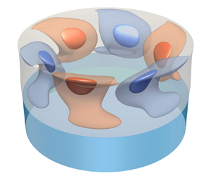
Figure 1. Schematic of the problem set-up and coordinates. The hot (red) and cold (blue) solid rods supporting the liquid bridge (light blue) are mounted coaxially in a closed cylindrical gas container (grey, hatched). Gravity acts in the negative  $z$ direction and leads to the hydrostatic shape $h(z)$ of the liquid bridge. The system is axisymmetric with respect to the dash-dotted line ( $r=0$).
While the cylindrical sidewall and the annular top and bottom walls of the chamber are assumed to be adiabatic, the cylindrical support rods are kept at different but constant temperatures  $T_{hot}=T_0+\Delta T/2$ and $T_{cold}=T_0-\Delta T/2$, respectively, where $T_0=(T_{hot}+T_{cold} )/2$ is the mean temperature, hereinafter used as the reference temperature. The enforced temperature variation across the liquid bridge creates a variation of the surface tension that can be described, to first order, by the linear dependence
 \begin{equation} \sigma(T)=\sigma_0-\gamma(T-T_0)+{O}[ \left(T-T_0 \right)^2 ], \end{equation}
where  $\sigma _0 = \sigma (T_0)$ is the surface tension at the mean temperature, and $\gamma =-\partial \sigma / \partial T |_{T=T_0}$ is the negative surface tension coefficient. The resulting surface tension gradients induce tangential shear stresses via the thermocapillary effect, which lead to an axisymmetric thermocapillary flow on both sides of the interface (Kuhlmann Reference Kuhlmann1999).
In addition to the thermocapillary stresses, the flow in the liquid is driven by buoyancy forces due to the temperature dependence of the density of the liquid:
 \begin{equation} \rho (T) = \rho_0\{1-\beta (T-T_0 )+{O}[ (T-T_0 )^2 ] \}, \end{equation}
where  $\rho _0=\rho (T_0)$ is the liquid density at the reference temperature, and $\beta = -\rho _0^{-1}(\partial \rho / \partial T)_p$ is the thermal expansion coefficient. Buoyancy forces also act in the gas phase due to the temperature-induced density variation of the gas in contact with the liquid–gas interface. For short liquid bridges employed in terrestrial laboratories, thermocapillary surface forces typically dominate over buoyant volume forces.
2.2. Governing equations
To compute the axisymmetric flow and temperature fields, and to investigate the hydrodynamic stability of the flow, the governing transport equations must be solved subject to the respective boundary conditions.
2.2.1. Transport equations
To non-dimensionalise the governing equations, we adopt the thermocapillary diffusive scaling given in table 1 (see e.g. Kuhlmann Reference Kuhlmann1999), where  $\nu$ is the constant kinematic viscosity of the liquid at the reference temperature. The temperature dependence of the density in the liquid and in the gas is taken into account within the Oberbeck–Boussinesq approximation (Landau & Lifschitz Reference Landau and Lifschitz1959; Mihaljan Reference Mihaljan1962). In this formulation, the Navier–Stokes, continuity and energy equations for the liquid phase read
 $$\begin{gather} \frac{\partial \boldsymbol{u}}{\partial t} +{{Re}}\,\boldsymbol{u} \boldsymbol{\cdot} \boldsymbol{\nabla} \boldsymbol{u} ={-}\boldsymbol{\nabla} p +\nabla^2 \boldsymbol{u}+{{Bd}}\,\vartheta \boldsymbol{e}_z, \end{gather}$$
 $$\begin{gather}\boldsymbol{\nabla} \boldsymbol{\cdot} \boldsymbol{u} = 0, \end{gather}$$
 $$\begin{gather}\frac{\partial \vartheta}{\partial t} + {{Re}}\,\boldsymbol{u} \boldsymbol{\cdot} \boldsymbol{\nabla} \vartheta = \frac{1}{{{Pr}}}\,\nabla^2 \vartheta, \end{gather}$$
where  $\vartheta = (T-T_0)/\Delta T$ is the normalised deviation from the reference temperature. The fluid motion depends on the thermocapillary Reynolds, Prandtl and dynamic Bond numbers defined as
 \begin{equation} {{Re}}=\frac{\gamma\,\Delta T\,d}{\rho_0 \nu^2}, \quad {{Pr}} = \frac{\nu}{\kappa},\quad {{Bd}} = \frac{\rho_0 g\beta d^2}{\gamma}, \end{equation}
where  $\kappa$ is the constant thermal diffusivity of the liquid at the reference temperature. Instead of ${{Re}}$, the Marangoni number ${{Ma}}={{Re}}\,{{Pr}}$ can be used.
Table 1. Scaling.
Using the same scaling, the flow in the gas phase is governed by
 $$\begin{gather} \frac{\partial \boldsymbol{u}_{g}}{\partial t} + {{Re}}\,\boldsymbol{u}_{g} \boldsymbol{\cdot} \boldsymbol{\nabla} \boldsymbol{u}_{g} ={-}\frac{1}{\tilde{\rho}}\,\boldsymbol{\nabla} p_{g} +\tilde{\nu}\,\nabla^2 \boldsymbol{u}_{g} + \tilde\beta\,{{Bd}}\,\vartheta_{g} \boldsymbol{e}_z, \end{gather}$$
 $$\begin{gather}\boldsymbol{\nabla} \boldsymbol{\cdot} \boldsymbol{u}_{g} = 0, \end{gather}$$
 $$\begin{gather}\frac{\partial \vartheta_{g}}{\partial t} + {{Re}}\,\boldsymbol{u}_{g} \boldsymbol{\cdot} \boldsymbol{\nabla} \vartheta_{g} = \frac{\tilde{\kappa}}{{{Pr}}}\,\nabla^2 \vartheta_{g}, \end{gather}$$
where the non-dimensional field quantities are indicated by the subscript  ${g}$. The additional non-dimensional parameters are the gas-to-liquid ratios of the density $\tilde {\rho }=\rho _{g}/\rho _0$, the kinematic viscosity $\tilde {\nu }=\nu _{g}/\nu$, the thermal diffusivity $\tilde {\kappa }=\kappa _{g}/\kappa$, and the thermal expansion coefficient $\tilde \beta =\beta _{g}/\beta$. Introducing
 \begin{equation} \boldsymbol{\alpha} = \left( \alpha_\rho,\alpha_\nu,\alpha_\kappa,\alpha_\beta \right)= \begin{cases} (1,1,1,1), & \text{for the liquid phase},\\ (\tilde{\rho},\tilde{\nu},\tilde{\kappa},\tilde\beta), & \text{for the gas phase}, \end{cases} \end{equation}
allows us to refer to both phases at the same time, while keeping the notation succinct.
2.2.2. Boundary conditions
(i) Support rods. To be able to control experimentally the temperatures imposed on the liquid bridge, the heating rods are typically made from good thermal conductors. Accordingly, the surfaces of the rods are modelled as isothermal, no-slip and no-penetration walls,
 \begin{align} \text{hot rod: } & \quad \boldsymbol{u}=\boldsymbol{u}_{g} = 0, \quad \vartheta=\vartheta_{g}= 1/2, \end{align}
 \begin{align} \text{cold rod: }& \quad \boldsymbol{u}=\boldsymbol{u}_{g} = 0, \quad \vartheta=\vartheta_{g}={-} 1/2, \end{align}
being in contact with the liquid along the faces of the rods and with the gas phase along the cylindrical surface.
(ii) Chamber walls. The outer cylindrical wall and the top and bottom walls of the closed chamber are considered as no-slip and adiabatic boundaries satisfying
 \begin{align} r=\eta/\varGamma: & \quad \boldsymbol{u}_{g} =0, \quad \frac{\partial \vartheta_{g}}{\partial r}=0, \end{align}
 \begin{align} z={\pm} \left(1/2 + \varGamma_{rod}/\varGamma\right): & \quad \boldsymbol{u}_{g}=0, \quad \frac{\partial \vartheta_{g}}{\partial z}=0. \end{align}
 (iii) Liquid–gas interface. The contiguous non-axisymmetric liquid–gas interface is described by a unique radial position  $r=h(\varphi, z, t)$ on which coupling conditions for $\boldsymbol{u}$ and $\vartheta$ must be provided. The continuity of temperature and heat flux requires
 \begin{equation} r=h(\varphi, z, t) : \quad \vartheta = \vartheta_{g} \quad \text{and} \quad \boldsymbol{n}\boldsymbol{\cdot} \boldsymbol{\nabla} \vartheta = \tilde{\kappa} \boldsymbol{n}\boldsymbol{\cdot} \boldsymbol{\nabla} \vartheta_{g}, \end{equation}
where  $\boldsymbol {n}$ is the local unit vector normal to the interface directed from the liquid into the gas phase. The kinematic coupling
 \begin{equation} r=h(\varphi, z, t) : \quad \boldsymbol{u} = \boldsymbol{u}_{g} \quad \text{and} \quad u = \frac{1}{{{Re}}}\, \frac{\partial h}{\partial t} + \frac{v}{r}\,\frac{\partial h}{\partial \varphi} + w\,\frac{\partial h}{\partial z}, \end{equation}
forces material elements on the interface to remain on the interface. Finally, the dynamic condition provided by the tangential stress balance
 \begin{equation} r=h(\varphi, z, t) : \quad \boldsymbol{n}\boldsymbol{\cdot}\boldsymbol{\mathsf{S}}\boldsymbol{\cdot}\boldsymbol{t} ={-}\boldsymbol{\nabla} \vartheta \boldsymbol{\cdot}\boldsymbol{t}+\tilde{\rho}\tilde{\nu} \boldsymbol{n}\boldsymbol{\cdot}\boldsymbol{\mathsf{S}}_{g}\boldsymbol{\cdot}\boldsymbol{t} \end{equation}
must be satisfied, where  $\boldsymbol{\mathsf{S}}=\boldsymbol {\nabla }\boldsymbol {u}+(\boldsymbol {\nabla }\boldsymbol {u})^\mathrm {T}$ and $\tilde {\rho }\tilde {\nu }\boldsymbol{\mathsf{S}}_{g}$ are the viscous stress tensors in the liquid and the gas, respectively. The vector $\boldsymbol {t}$ can be any of the two orthogonal unit vectors tangent to the interface.
2.3. Solution structure
2.3.1. Shape of the interface
The non-dimensional radial position  $r=h(\varphi,z,t)$ of the interface is part of the solution and therefore a priori unknown. Motivated by the very small capillary numbers ${{Ca}} = \gamma \,\Delta T/\sigma _0$ in typical experiments, we consider the limit of asymptotically large mean surface tension $\sigma _0$ in which ${{Ca}} \to 0$. In this limit, dynamic free-surface deformations can be neglected, and the problem of determining the liquid–gas interface decouples from solving (2.4) and (2.6) together with (2.8)–(2.12). These circumstances allow for an axisymmetric and stationary interface $h(\varphi,z,t) \to h(z)$ that is determined solely by the normal-stress balance, yielding the Young–Laplace equation
 \begin{equation} \Delta p_h =\frac{\boldsymbol{\nabla} \boldsymbol{\cdot} \boldsymbol{n}}{{{Ca}}} +\frac{{{Bo}}}{{{Ca}}}\,z, \end{equation}
where  $\boldsymbol{n} = (1,0,-h_z)^\text {T}/\sqrt {1+h_z^2}$ is the outward surface normal vector, $\Delta p_h$ is the hydrostatic (subscript $h$) pressure jump across the liquid–gas interface, and
 \begin{equation} {{Bo}} = \frac{(\rho_0-\rho_{{g0}}) g d^2}{\sigma_0} \end{equation}
is the static Bond number. Note that the ratio  $\lambda ={{Bd}}/{{Bo}} = \rho _0\beta \sigma _0 / [\gamma (\rho _0-\rho _{{g0}})]$ is a material parameter. The Young–Laplace equation (2.13) for $h$ is of second order in $z$ and $\varphi$, and needs to be closed by additional conditions. The pinned contact lines require
 \begin{equation} h\left(z={\pm} 1/2 \right) = \frac{1}{\varGamma}. \end{equation}
Owing to these constraints, (2.13) has an axisymmetric solution  $h(z)$, which we consider within its stability limits (Slobozhanin & Perales Reference Slobozhanin and Perales1993). To determine $h(z)$ and the pressure jump $p_h$ uniquely, (2.13) is solved subject to the volume constraint
 \begin{equation} \varGamma^2\int_{{-}1/2}^{1/2} h^{2}(z)\, \mathrm{d} z={\mathcal{V}}, \end{equation}
where  ${\mathcal {V}}=V_l/V_0$ is the liquid volume $V_l$ normalised by the volume $V_0={\rm \pi} r_{i}^2 d$ of an upright cylindrical liquid bridge. Within the range of $\mathcal {V}$ considered, the contact angle is a bijective function of $\mathcal {V}$ (Nienhüser & Kuhlmann Reference Nienhüser and Kuhlmann2002).
2.3.2. Basic flow
For a given axisymmetric hydrostatic shape  $h(z)$ of the liquid bridge, the symmetries of the problem allow for a steady axisymmetric flow ( $\partial _t=\partial _\varphi =0$) with $v_0=v_{g0}=0$, which is denoted $\boldsymbol {q}_0(r,z)=(u_0,w_0,p_0,\vartheta _0)$ (liquid phase) and $\boldsymbol {q}_{{g0}}(r,z)=(u_{{g0}},w_{{g0}},p_{{g0}},\vartheta _{{g0}})$ (gas phase). The pressure fields $p_{g0}$ and $p_0$ are flow-induced and add, respectively, to the ambient pressures $p_a$ (gas) and $p_a+\Delta p_h$ (liquid).
The flows  $\boldsymbol {q}_0$ and $\boldsymbol {q}_{{g0}}$ are obtained by solving the steady axisymmetric versions of the differential equations (2.4) and (2.6), subject to the steady axisymmetric versions of the boundary conditions. On $r=0$, axisymmetry requires
 \begin{equation} u_0=\frac{\partial w_0}{\partial r}=\frac{\partial \vartheta_0}{\partial r}=0, \end{equation}
while on the free surface we obtain, from (2.11a,b),
 \begin{equation} \frac{u_0}{w_0}=h_z. \end{equation}
2.3.3. Linear stability analysis
For small Reynolds numbers  ${{Re}}$, the basic flow $(\boldsymbol {q}_{0},\boldsymbol {q}_{{g0}})$ is stable. When ${{Re}}$ exceeds a critical Reynolds number ${{Re}}_c$, the basic flow becomes unstable. In order to calculate the critical threshold, a linear stability analysis is carried out. To that end, the general three-dimensional time-dependent flow $\boldsymbol {q}=(u,v,w,p,\vartheta )$ and $\boldsymbol {q}_{g}=(u_{g},v_{g},w_{g},p_{g},\vartheta _{g})$ is written as
 \begin{align} u&= u_0(r,z)+u'(r,\varphi,z,t),& u_{g}&= u_{{g0}}(r,z)+u_{g}'(r,\varphi,z,t), \end{align}
 \begin{align} v&=0 + v'(r,\varphi,z,t),& v_{g}&= 0 +v_{g}'(r,\varphi,z,t), \end{align}
 \begin{align} w&= w_0(r,z)+w'(r,\varphi,z,t),& w_{g}&= w_{{g0}}(r,z)+w_{g}'(r,\varphi,z,t), \end{align}
 \begin{align} p&= p_0(r,z)+p'(r,\varphi,z,t),& p_{g}&= p_{{g0}}(r,z)+p_{g}'(r,\varphi,z,t), \end{align}
 \begin{align} \vartheta &=\vartheta_0(r,z)+\vartheta'(r,\varphi,z,t),& \vartheta_{g} &= \vartheta_{{g0}}(r,z)+\vartheta_{g}'(r,\varphi,z,t), \end{align}
where deviations from the basic flow are indicated by a prime  $(')$. Inserting this decomposition into (2.4) and (2.6), and linearising with respect to the perturbation quantities, yields the linear stability equations that have the same form,
 $$\begin{gather} \frac{\partial \boldsymbol{u}'}{\partial t} + {{Re}} (\boldsymbol{u}_0 \boldsymbol{\cdot} \boldsymbol{\nabla} \boldsymbol{u}'+ \boldsymbol{u}' \boldsymbol{\cdot} \boldsymbol{\nabla} \boldsymbol{u}_0) ={-}\frac{1}{\alpha_\rho}\,\boldsymbol{\nabla} p' +\alpha_\nu\,\nabla^2 \boldsymbol{u}'+\alpha_\beta\,{{Bd}}\, \vartheta' \boldsymbol{e}_z, \end{gather}$$
 $$\begin{gather}\boldsymbol{\nabla} \boldsymbol{\cdot} \boldsymbol{u}' = 0, \end{gather}$$
 $$\begin{gather}\frac{\partial \vartheta'}{\partial t} + {{Re}} (\boldsymbol{u}_0 \boldsymbol{\cdot} \boldsymbol{\nabla} \vartheta'+ \boldsymbol{u}' \boldsymbol{\cdot} \boldsymbol{\nabla} \vartheta_0) = \frac{\alpha_\kappa}{{{Pr}}}\,\nabla^2 \vartheta' , \end{gather}$$
for both phases. The subscript ‘g’ (for the gas phase) no longer appears, because the distinction between the two phases is made, henceforth, by the set of coefficients  $\boldsymbol{\alpha}$ defined in (2.7).
Due to the homogeneity of (2.20) in  $\varphi$ and $t$, the general solution $\boldsymbol {q}'=(u',v',w',p',\vartheta ')$ of (2.20) can be written as a superposition of normal modes
 \begin{equation} \boldsymbol{q}' = \sum_{j,m} \hat{\boldsymbol{q}}_{j,m}(r,z)\exp({\mu_{j,m} t+\mathrm{i} m\varphi})+\text{c.c.}, \end{equation}
where  $\mu = \mu _{j,m} \in \mathbb {C}$ is a complex growth rate, and $m\in \mathbb {N}_0$ is the azimuthal wavenumber. The index $j$ numbers the discrete part of the spectrum, and c.c. denotes the complex conjugate. Inserting the ansatz (2.21) into the linear perturbation equations (2.20), one obtains linear differential equations for the perturbation amplitudes $\hat {\boldsymbol {q}} = (\hat {u}, \hat {v}, \hat {w}, \hat {p}, \hat {\vartheta })$ that depend only on $r$ and $z$:
$z$:
 \begin{align}
&\mu\hat{u}+{{Re}}\left[ \left( \frac{1}{r}
+\frac{\partial }{\partial r} \right) (2u_0\hat{u})
+\frac{u_0 \mathrm{i} \hat{v}m}{r} +\frac{\partial (u_0
\hat{w}+\hat{u}w_0)}{\partial z}\right] \nonumber\\ &\qquad
={-}\frac{1}{\alpha_\rho}\,\frac{\partial \hat{p}}{\partial
r}+\alpha_\nu\left[ \frac{1}{r}\, \frac{\partial}{\partial
r} \left( r\,\frac{\partial \hat{u}}{\partial r}
\right)-(m^2+1)\,\frac{\hat{u}}{r^2}-\frac{2}{r^2}\,\mathrm{i}
\hat{v}m+\frac{\partial^2 \hat{u}}{\partial z^2}
\right], \\
&\mu\hat{v}+{{Re}}\left[\left( \frac{2}{r}
+\frac{\partial }{\partial r} \right) (u_0\hat{v})
+\frac{\partial (\hat{v}w_0)}{\partial z}\right]\nonumber\\
&\qquad
={-}\frac{1}{\alpha_\rho}\,\frac{1}{r}\,\hat{p}\mathrm{i}
m +\alpha_\nu\left[ \frac{1}{r}\, \frac{\partial}{\partial
r} \left( r\,\frac{\partial \hat{v}}{\partial r}
\right)-(m^2+1)\,\frac{\hat{v}}{r^2}+\frac{2}{r^2}\,\mathrm{i}
\hat{u}m+\frac{\partial^2 \hat{v}}{\partial z^2} \right],\\
&
\mu\hat{w}+{{Re}}\left[\frac{1}{r}\,\frac{\partial
(w_0 \hat{u}+\hat{w}u_0)}{\partial r} +\frac{w_0 \mathrm{i}
\hat{v}m}{r} + 2\,\frac{\partial w_0\hat{w}}{\partial
z}\right]\nonumber\\ &\qquad
={-}\frac{1}{\alpha_\rho}\,\frac{\partial \hat{p}}{\partial
z}+\alpha_\nu\left[ \frac{1}{r}\, \frac{\partial}{\partial
r} \left( r\,\frac{\partial \hat{w}}{\partial r}
\right)-m^2\,\frac{\hat{w}}{r^2}+\frac{\partial^2
\hat{w}}{\partial z^2}
\right]+\alpha_\beta\,{{Bd}}\,\hat{\vartheta},
\end{align}
\begin{align}
&\mu\hat{u}+{{Re}}\left[ \left( \frac{1}{r}
+\frac{\partial }{\partial r} \right) (2u_0\hat{u})
+\frac{u_0 \mathrm{i} \hat{v}m}{r} +\frac{\partial (u_0
\hat{w}+\hat{u}w_0)}{\partial z}\right] \nonumber\\ &\qquad
={-}\frac{1}{\alpha_\rho}\,\frac{\partial \hat{p}}{\partial
r}+\alpha_\nu\left[ \frac{1}{r}\, \frac{\partial}{\partial
r} \left( r\,\frac{\partial \hat{u}}{\partial r}
\right)-(m^2+1)\,\frac{\hat{u}}{r^2}-\frac{2}{r^2}\,\mathrm{i}
\hat{v}m+\frac{\partial^2 \hat{u}}{\partial z^2}
\right], \\
&\mu\hat{v}+{{Re}}\left[\left( \frac{2}{r}
+\frac{\partial }{\partial r} \right) (u_0\hat{v})
+\frac{\partial (\hat{v}w_0)}{\partial z}\right]\nonumber\\
&\qquad
={-}\frac{1}{\alpha_\rho}\,\frac{1}{r}\,\hat{p}\mathrm{i}
m +\alpha_\nu\left[ \frac{1}{r}\, \frac{\partial}{\partial
r} \left( r\,\frac{\partial \hat{v}}{\partial r}
\right)-(m^2+1)\,\frac{\hat{v}}{r^2}+\frac{2}{r^2}\,\mathrm{i}
\hat{u}m+\frac{\partial^2 \hat{v}}{\partial z^2} \right],\\
&
\mu\hat{w}+{{Re}}\left[\frac{1}{r}\,\frac{\partial
(w_0 \hat{u}+\hat{w}u_0)}{\partial r} +\frac{w_0 \mathrm{i}
\hat{v}m}{r} + 2\,\frac{\partial w_0\hat{w}}{\partial
z}\right]\nonumber\\ &\qquad
={-}\frac{1}{\alpha_\rho}\,\frac{\partial \hat{p}}{\partial
z}+\alpha_\nu\left[ \frac{1}{r}\, \frac{\partial}{\partial
r} \left( r\,\frac{\partial \hat{w}}{\partial r}
\right)-m^2\,\frac{\hat{w}}{r^2}+\frac{\partial^2
\hat{w}}{\partial z^2}
\right]+\alpha_\beta\,{{Bd}}\,\hat{\vartheta},
\end{align}
 \begin{align}
&\frac{1}{r}\,\frac{\partial (r \hat{u})}{\partial
r}+\frac{1}{r}\,\mathrm{i}\hat{v}m+\frac{\partial
\hat{w}}{\partial z}=0,\end{align}
\begin{align}
&\frac{1}{r}\,\frac{\partial (r \hat{u})}{\partial
r}+\frac{1}{r}\,\mathrm{i}\hat{v}m+\frac{\partial
\hat{w}}{\partial z}=0,\end{align}
 \begin{align}
&\mu\hat{\vartheta}+{{Re}}\left[\frac{1}{r}\,\frac{\partial
(\vartheta_0 \hat{u}+\hat{\vartheta}u_0)}{\partial r}
+\frac{\vartheta_0 \mathrm{i} \hat{v}m}{r} + \frac{\partial
( \vartheta_0\hat{w}+\hat{\vartheta}w_0)}{\partial
z}\right]\nonumber\\
&\qquad
=\frac{\alpha_\kappa}{{{Pr}}}\left[
\frac{1}{r}\,\frac{\partial}{\partial r} \left(
r\,\frac{\partial \hat{\vartheta}}{\partial r}
\right)-m^2\,\frac{\hat{\vartheta}}{r^2}+\frac{\partial^2
\hat{\vartheta}}{\partial z^2} \right].
\end{align}
\begin{align}
&\mu\hat{\vartheta}+{{Re}}\left[\frac{1}{r}\,\frac{\partial
(\vartheta_0 \hat{u}+\hat{\vartheta}u_0)}{\partial r}
+\frac{\vartheta_0 \mathrm{i} \hat{v}m}{r} + \frac{\partial
( \vartheta_0\hat{w}+\hat{\vartheta}w_0)}{\partial
z}\right]\nonumber\\
&\qquad
=\frac{\alpha_\kappa}{{{Pr}}}\left[
\frac{1}{r}\,\frac{\partial}{\partial r} \left(
r\,\frac{\partial \hat{\vartheta}}{\partial r}
\right)-m^2\,\frac{\hat{\vartheta}}{r^2}+\frac{\partial^2
\hat{\vartheta}}{\partial z^2} \right].
\end{align}
Using polar coordinates, the perturbation flow must satisfy boundary conditions on the axis  $r=0$. These are provided in table 2 and can be derived from uniqueness conditions for $\partial \boldsymbol {u}/\partial \varphi$ and $\partial \vartheta /\partial \varphi$ as $r\to 0$ (Batchelor & Gill Reference Batchelor and Gill1962; Xu & Davis Reference Xu and Davis1984). Since the imposed constant temperatures on the cylindrical rods are taken care of by the basic flow, all perturbation quantities must vanish on the support rods:
 \begin{equation} \hat{\boldsymbol{u}}=\hat{\boldsymbol{u}}_{g} = 0 \quad\text{and}\quad \hat{\vartheta}=\hat{\vartheta}_{g} = 0. \end{equation}
Like the basic flow, the velocity and heat flux of the perturbations must vanish on the solid adiabatic walls of the gas container:
 \begin{equation} \hat{\boldsymbol{u}}_{g} = 0 \quad\text{and}\quad \boldsymbol{n}\boldsymbol{\cdot}\boldsymbol{\nabla} \hat\vartheta_{g}=0. \end{equation}
In the limit  ${{Ca}}\to 0$ considered, the liquid–gas interface is indeformable. From (2.10a,b)–(2.12), the coupling on the axisymmetric interface at $r=h(z)$ between the liquid- and gas-phase perturbations is provided by
 \begin{equation} \hat{\boldsymbol{u}}=\hat{\boldsymbol{u}}_{g},\quad \hat{\vartheta} = \hat{\vartheta}_{g}, \quad \boldsymbol{n}\boldsymbol{\cdot} \boldsymbol{\nabla} \hat{\vartheta} = \tilde{\kappa} \boldsymbol{n}\boldsymbol{\cdot} \boldsymbol{\nabla} \hat{\vartheta}_{g} \quad \text{and}\quad \boldsymbol{n}\boldsymbol{\cdot}\hat{\boldsymbol{\mathsf{S}}}\boldsymbol{\cdot}\boldsymbol{t} ={-}\boldsymbol{\nabla} \hat{\vartheta} \boldsymbol{\cdot}\boldsymbol{t}+\tilde\rho\tilde{\nu} \boldsymbol{n}\boldsymbol{\cdot}\hat{\boldsymbol{\mathsf{S}}}_{g}\boldsymbol{\cdot}\boldsymbol{t}, \end{equation}
with  $\hat {\boldsymbol{\mathsf{S}}}=\boldsymbol {\nabla } \hat {\boldsymbol {u}}+(\boldsymbol {\nabla } \hat {\boldsymbol {u}})^\mathrm {T}$.
Table 2. Boundary conditions for the perturbation flow on  $r=0$.

For each azimuthal wavenumber  $m$, (2.22)–(2.25a–d) represent a linear eigenvalue problem with an infinite number of eigenmodes $\boldsymbol {q}'$. The eigenmodes and the corresponding eigenvalues
 \begin{align} \mu_{j,m} = \mu(j, m; {{Re}}, \varGamma, {\mathcal{V}}, {{Pr}}, \lambda, \tilde{\rho}, \tilde{\nu}, \tilde{\kappa}, \tilde\beta) \end{align}
depend on a number of parameters. Neutral values  ${{Re}}_n$ (using subscript $n$) of the Reynolds number associated with each mode $(j,m)$ are characterised by a vanishing real part (Re) of the eigenvalue, $\mathrm {Re} [\mu _{j,m} ({{Re}}_n)] = 0$. These conditions define neutral hypersurfaces ${{Re}}_n^{j,m}(\varGamma, {\mathcal {V}}, {{Pr}}, \lambda, \tilde {\rho }, \tilde {\nu }, \tilde {\kappa },\tilde \beta )$ in the parameter space. The envelope of all neutral hypersurfaces ${{Re}}_c = \min _{j,m}{{Re}}_n^{j,m}$ is the critical Reynolds number ${{Re}}_c(\varGamma, {\mathcal {V}}, {{Pr}}, \lambda, \tilde {\rho }, \tilde {\nu }, \tilde {\kappa },\tilde \beta )$. For slightly supercritical Reynolds numbers with $\epsilon = ({{Re}}-{{Re}}_c)/{{Re}}_c \ll 1$, the basic flow is guaranteed to be unstable, because at least one eigenmode exists that has a positive growth rate $\mathrm {Re}(\mu ) > 0$. This does not preclude the rare case of isolated islands in parameter space for larger Reynolds numbers ( ${{Re}}/{{Re}}_c > 1$) for which the basic flow can be linearly stable, i.e. for which $\forall _{j,m}\,\mathrm {Re}(\mu _{j,m}) < 0$. However, within the present linear stability approach, which does not take care of nonlinear effects in the perturbation flow, it cannot be decided if the basic flow $\boldsymbol{q}_0$ is stable to finite-amplitude perturbations, either in these linearly stable islands or for ${{Re}} < {{Re}}_c$. Experimental and numerical evidence (Velten et al. Reference Velten, Schwabe and Scharmann1991; Leypoldt et al. Reference Leypoldt, Kuhlmann and Rath2000; Sim & Zebib Reference Sim and Zebib2002) suggests, however, that the first instability of the basic flow is typically supercritical.
2.4. Post-processing
Analysing the energy transfer between the basic flow and the neutral mode can provide insights regarding the instability mechanism and helps us to understand the underlying physics. To that end, we build on the energy analysis derived in Nienhüser & Kuhlmann (Reference Nienhüser and Kuhlmann2002) for a non-cylindrical axisymmetric liquid bridge, where the gas phase was neglected, and extend the equations to the present two-phase model. Multiplying the linearised momentum equation (2.20a) by the perturbation velocity vector  $\boldsymbol {u}'$, the resulting equations for the liquid and gas are integrated over the volumes $V_l$ and $V_{g}$, respectively, occupied by each phase. After splitting all terms into volume and surface integrals by means of Green's theorem, we obtain the balance
 \begin{equation} \frac{\mathrm{d} E_{kin}}{\mathrm{d} t}= \frac{1}{\mathcal{D}_{kin}}\,\frac{\mathrm{d}}{\mathrm{d} t}\int_{V_i}\frac{\boldsymbol{u}'^2}{2}\,\mathrm{d} V ={-}1 + M_r + M_\varphi + M_z + \sum_{j=1}^5 I_j + B,\quad i\in [{l},{g}], \end{equation}
for the (normalised) rate of change of the kinetic energy  $E_{kin}$, where all terms on the right-hand side have been normalised by the mechanical dissipation rate $\mathcal {D}_{kin}$. Similarly, multiplication of (2.20c) by $\vartheta '$ and integration over the volume occupied by each phase yields the thermal energy balance
 \begin{equation} \frac{\mathrm{d} E_{th}}{\mathrm{d} t}= \frac{1}{\mathcal{D}_{th}}\,\frac{\mathrm{d}}{\mathrm{d} t}\int_{V_i}\frac{\vartheta'^2}{2}\,\mathrm{d} V ={-}1 + \sum_{j=1}^2 J_j + H_{fs},\quad i\in [{l},\,{g}], \end{equation}
where all terms now have been scaled by the thermal dissipation rate  $\mathcal {D}_{th}$. Thus the scaled dissipation rates $D_{kin} = D_{th} = 1$ are constant. The subscripts ${l}$ and ${g}$ have been omitted for all terms arising in (2.27) and (2.28) with the understanding that the balances are valid separately for both the liquid and gas phases. Detailed expressions for the individual terms are provided in Appendix A. The terms $\sum I_j = \sum \int i_j \, \mathrm {d} V$ and $\sum J_j = \sum \int j_j \, \mathrm {d} V$ (see (A2)) represent the scaled total production rates of kinetic and thermal energy, respectively, which is transferred between the basic and perturbation flows, with corresponding local production densities $i_j$ and $j_j$. The terms $M_r$, $M_\varphi$ and $M_z$ in the kinetic energy balance (2.27) represent the work done per unit time by Marangoni forces in the respective spatial directions. Furthermore, the contribution $B$ (see (A4)) accounts for the work done per unit time by buoyancy forces. In the thermal budget (2.28), $H_{fs}$ (see (A5)) denotes the heat transferred through the liquid–gas interface. It appears in the budgets for both the liquid and gas phases, albeit with opposite signs.
It is generally accepted to refer to  $E_{th}$ and $E_{{th},{g}}$ as thermal energies, even though it contradicts the definition of the thermodynamic thermal energy. Hence, what we call thermal energy is rather a measure for the temperature deviation from the axisymmetric temperature field.
2.5. Reference case and parameter variation
Due to the large number of parameters governing the linear stability problem, it is computationally too demanding to cover the whole parameter space. Therefore, we consider the liquid–gas couple made of 2 cSt silicone oil (KF96L-2cs, Shin-Etsu Chemical Co., Ltd., Japan) and air with constant material parameters, evaluated at  $T_0=25\,^\circ$C for both fluids. This selection determines the non-dimensional material parameters ${{Pr}}$, $\lambda$, $\tilde {\rho }$, $\tilde {\nu }$, $\tilde {\kappa }$ and $\tilde \beta$. The thermophysical properties of both working fluids are listed in table 3.
Table 3. Thermophysical properties of the working fluids 2 cSt silicone oil KF96L-2cs and air at  $25\,^\circ$C.

Furthermore, we keep the aspect ratio of the support rods as well as the chamber radius ratio constant at  $\varGamma _{rod}=0.4$ and $\eta =4$, respectively. This configuration corresponds to the experiments carried out by Romanò et al. (Reference Romanò, Kuhlmann, Ishimura and Ueno2017). We are left with the important geometrical parameters $\mathcal {V}$ and $\varGamma$ representing the volume of liquid and the geometric aspect ratio of the liquid bridge, respectively. Finally, the gravity level can be varied via the Bond number ${{Bd}}$.
The origin of all parameter variations is a common reference case. It is based on the experimental geometry investigated by Romanò et al. (Reference Romanò, Kuhlmann, Ishimura and Ueno2017) with support rods of radius  $r_{i}=2.5$ mm and terrestrial gravity. Different from our objectives, however, Romanò et al. (Reference Romanò, Kuhlmann, Ishimura and Ueno2017) kept the temperature difference constant at $\Delta T=10\,\text {K} <\Delta T_c$, which is far subcritical. We define the reference case by $\varGamma _{ref}=0.66$, ${\mathcal {V}}_{ref} =1$ and ${{Bd}}_{ref}=0.41$. All reference parameters are collected in table 4. Starting from the reference case, we perform three parameter variations.
(i) A first variation, which is typically made in laboratory experiments, is a variation of the length $d$ of the liquid bridge (Velten et al. Reference Velten, Schwabe and Scharmann1991; Monti, Savino & Lappa Reference Monti, Savino and Lappa2000; Nienhüser & Kuhlmann Reference Nienhüser and Kuhlmann2003; Melnikov et al. Reference Melnikov, Shevtsova, Yano and Nishino2015), corresponding to a variation of $\varGamma$. Owing to the dependence of ${{Bd}}\sim d^2$, we simultaneously vary ${{Bd}}$ such that ${{Bd}} = {{Bd}}_{ref}(\varGamma /\varGamma _{ref})^2$, corresponding to a constant acceleration of gravity. The range of variation is $\varGamma \in [0.5, 1.8]$ and ${{Bd}} \in [0.236, 3.07]$.
(ii) In a second series of calculations, we vary
${\mathcal {V}} \in [0.65, 1.3]$ for $\varGamma =\varGamma _{ref}$ and ${{Bd}}={{Bd}}_{ref}$. This type of variation has also been used in experiments (Hu et al. Reference Hu, Shu, Zhou and Tang1994; Sakurai et al. Reference Sakurai, Ohishi and Hirata1996; Tang & Hu Reference Tang and Hu1999; Nienhüser & Kuhlmann Reference Nienhüser and Kuhlmann2002; Yano et al. Reference Yano, Maruyama, Matsunaga and Nishino2016).(iii) In a third step, we vary the acceleration of gravity for
$\varGamma =\varGamma _{ref}$ and ${\mathcal {V}}={\mathcal {V}}_{ref}$. In this series of calculations, the Bond number is varied in the range ${{Bd}} \in [-1.25, 1.25]$. This variation is intended to show how the instabilities for heating from above (reference case) and below are related to each other and to the case of zero gravity in which buoyancy forces and hydrostatic pressure are eliminated (Velten et al. Reference Velten, Schwabe and Scharmann1991; Wanschura, Kuhlmann & Rath Reference Wanschura, Kuhlmann and Rath1997b; Kawamura et al. Reference Kawamura, Nishino, Matsumoto and Ueno2012).


Table 4. Constant non-dimensional parameters;  $\varGamma$, ${\mathcal {V}}$ and ${{Bd}}$ are varied around the reference values given.
3. Numerical methods
To compute the basic state and its linear stability, a revised version of the numerical code MaranStable (Kuhlmann, Lukasser & Muldoon Reference Kuhlmann, Lukasser and Muldoon2011; Stojanovic & Kuhlmann Reference Stojanovic and Kuhlmann2020b) is used. It is based on an earlier version developed by M. Lukasser (see § 4.2 of Shevtsova et al. Reference Shevtsova, Gaponenko, Kuhlmann, Lappa, Lukasser, Matsumoto, Mialdun, Montanero, Nishino and Ueno2014).
3.1. Shape of the interface
In a first step, the static axisymmetric shape  $h(z)$ of the liquid–gas interface is computed. To that end, the Young–Laplace equation (2.13) is reformulated as a system of two ordinary differential equations:
 $$\begin{gather} h_{zz}=(1+h_z^2)\left[\frac{1}{h}-({{Ca}}\,\Delta p_h-{{Bo}}\,z)\sqrt{1+h_z^2}\right], \end{gather}$$
 $$\begin{gather}\Delta p_{h,z}=0, \end{gather}$$
where the subscript  $z$ denotes differentiation with respect to $z$. These equations, together with the pinning conditions (2.15), represent a boundary value problem, which is discretised by central finite differences on a uniform mesh. The pressure jump $\Delta p_h$ is determined by the volume constraint (2.16). The discretised set of nonlinear equations is solved using the Newton–Raphson method. The iteration is terminated as soon as both the $L_\infty$ and $L_2$ norms of the residual have dropped below $10^{-6}$.
3.2. Basic flow
The steady axisymmetric versions of the nonlinear equations (2.4) and (2.6) determining the basic state are discretised on a structured and staggered grid using second-order finite volumes (Wesseling Reference Wesseling2009). In order to implement the boundary conditions on the liquid–gas interface, the grid is body-fitted to the interface, transforming the radial coordinate to  $\xi = r/h(z)$. To perform this transformation, the previously determined $h(z)$ is interpolated to the current grid using splines. Furthermore, the grid is refined towards all boundaries using a hyperbolic-tangent profile (Thompson, Warsi & Mastin Reference Thompson, Warsi and Mastin1985). Inside the liquid, a minimum cell width of $\Delta _{{min},{l}} = 5\times 10^{-5}$ was chosen for the wall-bounded cells and along the interface in order to guarantee that thermal boundary layers will be resolved for all calculations. On the axis of symmetry (subscript $a$), moderate temperature and velocity gradients are expected, justifying the larger minimum cell width in radial direction $\Delta _{{min},a} = 10^{-3}$. The spatial resolution in the gas phase was set to $\Delta _{{min},g}=3\Delta _{{min},l}$ along the interface, and $\Delta _{{min},c} = 10^{-3}\times \varGamma _{rod}/\varGamma$ close to the adiabatic chamber walls (subscript $c$). The cells are stretched towards the interior with a stretching factor $f=1.15$ until maximum cell widths $\Delta _{{max},{l}} = 0.0075 = 150\,\Delta _{{min},{l}}$ and $\Delta _{{max},{g}} = 0.02(\eta -1)/\varGamma = 150\,\Delta _{{min},{c}}\approx 600\,\Delta _{{min},{g}}$ are reached in the bulk of the liquid and the gas, respectively. These conditions lead to a total of $N_{tot} = 103\,613$ cells, of which $N_r\times N_z = 244\times 197$ cells belong to the liquid, and $N_r\times N_z =115\times 483$ cells belong to the gas phase. Figure 2 shows the physical mesh, but at much lower resolution than used for the actual calculations.

Figure 2. Example for the physical mesh inside the liquid (light blue) and the gas (grey). For better visualisation, the total number of nodes was reduced to  $N_{tot}=18\,852$, which is a reduction of more than 80 % compared to the mesh used for the calculations.
The nonlinear algebraic equations resulting from the discretisation are solved by Newton–Raphson iteration:
 $$\begin{gather} \boldsymbol{\mathsf{J}}(\boldsymbol{q}_0^{(k)})\boldsymbol{\cdot} \delta \boldsymbol{q} ={-}\boldsymbol{f}(\boldsymbol{q}_0^{(k)}), \end{gather}$$
 $$\begin{gather}\boldsymbol{q}_0^{(k+1)} = \boldsymbol{q}_0^{(k)} + \delta \boldsymbol{q}, \end{gather}$$
where  $\delta \boldsymbol {q}$ is the increment of the approximation of the basic flow from the $k$th to the $(k+1)$th iteration step. Inserting (3.2b) into the steady axisymmetric versions of (2.4) and (2.6) yields the equations governing $\delta \boldsymbol {q}$:
 $$\begin{gather} {{Re}}(\delta \boldsymbol{u} \boldsymbol{\cdot} \boldsymbol{\nabla} \boldsymbol{u}_0^{(k)} + \boldsymbol{u}_0^{(k)} \boldsymbol{\cdot} \boldsymbol{\nabla} \delta \boldsymbol{u}) + \frac{1}{\alpha_\rho}\, \boldsymbol{\nabla} \delta p - \alpha_\nu\,\nabla^2 \delta \boldsymbol{u} - \alpha_\beta\,{{Bd}}\, \delta \vartheta\,\boldsymbol{e}_z \nonumber\\ ={-}{{Re}}\,\boldsymbol{u}_0^{(k)} \boldsymbol{\cdot} \boldsymbol{\nabla} \boldsymbol{u}_0^{(k)} - \frac{1}{\alpha_\rho}\,\boldsymbol{\nabla} p_0^{(k)} + \alpha_\nu\,\nabla^2 \boldsymbol{u}_0^{(k)} + \alpha_\beta\,{{Bd}}\, \vartheta_0^{(k)}\,\boldsymbol{e}_z, \end{gather}$$
 $$\begin{gather}\boldsymbol{\nabla} \boldsymbol{\cdot} \delta \boldsymbol{u} ={-}\boldsymbol{\nabla} \boldsymbol{\cdot} \boldsymbol{u}_0^{(k)}, \end{gather}$$
 $$\begin{gather}\delta \boldsymbol{u} \boldsymbol{\cdot} \boldsymbol{\nabla} \vartheta_0^{(k)} + \boldsymbol{u}_0^{(k)} \boldsymbol{\cdot} \boldsymbol{\nabla} \delta \vartheta - \frac{\alpha_k}{{{Ma}}}\,\nabla^2 \delta \vartheta ={-}\boldsymbol{u}_0^{(k)} \boldsymbol{\cdot} \boldsymbol{\nabla} \vartheta_0^{(k)} + \frac{\alpha_k}{{{Ma}}}\,\nabla^2 \vartheta_0^{(k)}, \end{gather}$$
where the nonlinear terms have been linearised with respect to  $\delta \boldsymbol{q}$. The Jacobian operator $\boldsymbol{\mathsf{J}}(\boldsymbol {q}_0^{(k)})$ and the nonlinear residual $-\boldsymbol {f}(\boldsymbol {q}_0^{(k)})$ are identified readily from (3.3). The Newton iteration (3.2) is considered converged as soon as both the infinity norm $\|\delta \boldsymbol {q}\|_\infty$ and the $L_2$ norm $\|\delta \boldsymbol {q}\|_2$ of the residual have dropped below $10^{-6}$.
3.3. Linear stability of the basic flow
Once the basic state  $\boldsymbol{q}_0$ is computed, it parametrically enters the linear stability equations (2.22), which are discretized on the same mesh using the same finite volume method. The resulting large generalised complex eigenvalue problem is converted into a generalised eigenvalue problem with real matrices by introducing $\check v = \mathrm {i}\hat v$ (Theofilis Reference Theofilis2003). Defining the decay rate $\chi = -\mu$, the generalised real eigenvalue problem has the form
 \begin{equation} \boldsymbol{\mathsf{A}}\boldsymbol{\cdot}\hat{\boldsymbol{q}} = \chi \boldsymbol{\mathsf{B}}\boldsymbol{\cdot}\hat{\boldsymbol{q}}, \end{equation}
where  $\boldsymbol{\mathsf{B}}$ is singular. For a Reynolds number ${{Re}}\approx {{Re}}_n$ close to a neutral stability boundary (subscript $n$), the most dangerous modes (numbered by $i$) belong to the eigenvalues $\chi _i$ with the smallest real parts, satisfying $\mathrm {Re}{(\chi _i)}\approx 0$. To find the most dangerous eigenvalue, i.e. the one with the smallest real part of $\chi$, twelve eigenvalues $\tilde {\chi }_i$ with the smallest absolute value are computed, in a first step, via an implicitly restarted Arnoldi method implemented in ARPACK (Lehoucq, Sorensen & Yang Reference Lehoucq, Sorensen and Yang1998) and available under MATLAB. A Krylov subspace of dimension $K=100$ is employed. Based on the eigenvalue $\tilde {\chi }_{sr}$ with the smallest real part among the twelve eigenvalues $\tilde {\chi }_i$, i.e. $\tilde {\chi }_{sr} : \mathrm {Re}{(\tilde {\chi }_{sr})} = \min [\mathrm {Re}{(\tilde {\chi }_i)}]$, we adopt the method proposed by Meerbergen, Spence & Roose (Reference Meerbergen, Spence and Roose1994) to validate that the eigenvalue $\tilde {\chi }_{sr}$ is indeed the one with the smallest real part among all the eigenvalues $\chi _i$ and not only among the twelve eigenvalues $\tilde {\chi }_i$ with the smallest absolute value. To that end, 17 eigenvalues $\zeta =(\chi -a_2)(\chi -a_1)$ with the largest magnitude of the Cayley transform
 \begin{equation} (\boldsymbol{\mathsf{A}} - a_2\boldsymbol{\mathsf{B}})\boldsymbol{\cdot}\hat{\boldsymbol{q}} = \zeta (\boldsymbol{\mathsf{A}}-a_1 \boldsymbol{\mathsf{B}})\boldsymbol{\cdot}\hat{\boldsymbol{q}} \end{equation}
are computed, as described in Meerbergen et al. (Reference Meerbergen, Spence and Roose1994). The parameters  $a_1$ and $a_2$ are determined by the five real eigenvalues with the smallest absolute value and a user-defined parameter $b= \vert (\chi _i - a_2)/(\chi _i - a_2)\vert =1.2$, where $\chi _i$ is one of the eigenvalues with the smallest real part. The resulting 17 eigenvalues containing the most dangerous mode are then sorted according to the magnitudes of their real parts.
At the neutral Reynolds number  ${{Re}}_n$, the real part of the eigenvalue of the most dangerous mode, identified from the above procedure, crosses zero. To determine ${{Re}}_n$ for a given azimuthal wavenumber $m$, the Reynolds number is varied in small steps, typically by approximately 5 % of its value, until the sign of $\min _i {\rm Re} (\chi _i )\rvert _{m}$ changes, signalling that at least one root exists within this interval of ${{Re}}$. The root ${{Re}}_n$ is then computed by the bisected direct quadratic regula falsi as described in Gottlieb & Thompson (Reference Gottlieb and Thompson2010), using the convergence condition $|{\min _i \mathrm {Re}(\chi _i )\rvert _{m}} | < 10^{-5}$, i.e. a sufficiently small absolute value of the growth rate's real part. Repeating this procedure for a series of wavenumbers $m = 0,1,2, \ldots,M$ allows us to detect the critical Reynolds number ${{Re}}_c$ as the envelope gathering the lowest neutral Reynolds numbers over all ${{Re}}_n(m)$.
In order to track the neutral curves under a variation of one of the parameters  $\varGamma$, $\mathcal {V}$ or ${{Bd}}$, a natural continuation technique is used. The converged basic state and neutral Reynolds number are used as initial conditions for the Newton iteration to compute the basic state for the incremented parameter, followed by solving the new eigenvalue problem. The step change of the parameter is typically 1 % of its value. If necessary, the parameter variation is refined, e.g. near intersection points of neutral curves or when ${{Re}}_n$ depends sensitively on the parameter varied.
The numerical code has been tested extensively. Grid convergence, verification and validation are described in detail in Appendix B.
4. Results
4.1. Reference case
4.1.1. Basic flow
Since the basic two-dimensional flow enters the linear stability analysis parametrically, it is important to examine its characteristics closely. Figure 3 shows the streamlines and the temperature field at criticality for the reference case ( $\varGamma =0.66$, ${\mathcal {V}} =1$, ${{Bd}}=0.41$). The hydrostatic shape of the interface deviates only slightly from the cylindrical shape. The thermocapillary stresses along the interface, directed from the hot corner to the cold one, lead to a streamline crowding at the interface and drive a clockwise vortex in the liquid phase (figure 3). Even though the absolute Rayleigh number for the liquid phase is $|{{Ra}}| = |{{Pr}}\,{{Bd}}\,{{Re}}| = 8392$, buoyancy forces do not cause the instability, because of the overall stable thermal stratification (see also Wanschura et al. Reference Wanschura, Kuhlmann and Rath1997b). Buoyancy forces are, however, responsible for the vortex in the liquid, which is more slender than under zero gravity, because the hot fluid transported near the free surface to the cold wall has the tendency to rise in the bulk. This causes the large separation bubble on the cold wall (Romanò & Kuhlmann Reference Romanò and Kuhlmann2018), also visible in figure 3.

Figure 3. Streamlines and temperature fields  $\vartheta _0$ and $\vartheta _{{g0}}$ (colour) of the basic state for the reference case ( $\varGamma =0.66$, ${\mathcal {V}} =1$, ${{Bd}}=0.41$) at criticality ${{Re}}_c = 731$. Streamline levels differ in the liquid and the gas, but they are drawn equidistantly in each phase.
Owing to the geometry of the gas space, a much larger vortex is created in the gas phase (counterclockwise in figure 3). Because the thermal diffusivity of the gas is much higher than that of the liquid (table 4), the convective effect on the temperature distribution in the gas phase is very weak. The temperature distribution along the interface (figure 4), being larger than  $T_0$ on average, causes a mean temperature $\vartheta _{g0} > 0$ in the gas phase far away from the liquid bridge. Furthermore, a weak flow arises in a large separation bubble, while much smaller viscous eddies can be identified close to all four corners of the annular gas container. Buoyancy in the gas phase is even weaker than in the liquid phase. The ratio ${{Ra}}_{g}/{{Ra}} = \tilde \beta \tilde d^3/(\tilde \nu \tilde \kappa ) \approx 10^{-2}$, where $\tilde d= 1+2\varGamma _{rod}/\varGamma$, suggests that buoyancy is negligible in the gas.

Figure 4. Tangential velocity  $u_{t0}=\boldsymbol {t}\boldsymbol {\cdot }\boldsymbol {u}_0$ (solid blue lines) and temperature distribution $\vartheta _0$ (solid red lines) of the basic flow along the free surface (parametrised by $z$) for the reference case at criticality ( $\varGamma =0.66$, ${\mathcal {V}}=1$, ${{Bd}}=0.41$, ${{Re}}={{Re}}_c=731$). Also shown, as dashed lines, are the corresponding profiles for the single-fluid model at the same Reynolds number, and for an adiabatic free surface, neglecting viscous stresses from the gas. (a) Profiles along the whole free surface. (b) Zoom into the red rectangle shown in (a). The black curve indicates the shape $h(z)$ of the interface.
The distributions of the velocity (blue) and temperature (red) on the free surface are shown in figure 4(a) for the reference case (solid lines). Also shown are the profiles for the single-fluid model with an adiabatic free surface (dashed lines), neglecting viscous stresses from the gas. For both models, the boundary layer character is obvious from the steep variation of the temperature near the hot and cold corners. Associated with the temperature gradients are peaks of the surface velocity very close to the hot and cold corners. Of these, the cold-corner peak is particularly sharp, because the fluid at the interface is accelerated towards the wall, where it must get decelerated to zero. Since the finite volume method employed does not require any regularisation of the boundary conditions near the corners, the velocity peaks are fully resolved (zoom in figure 4b). The temperature is almost constant along the free surface midway between the two surface velocity peaks (figure 4b) as well as inside the main vortex in the liquid (figure 3). The two-fluid model exhibits a lower surface temperature in the plateau region than the adiabatic single-fluid model. This indicates that the two-fluid model exhibits a heat loss, i.e. a net heat flux outwards through the free surface (free-surface Nusselt number  ${{Nu}}_{fs}<0$ defined in (B2)), a stronger thermocapillary driving along the hotter part of the interface as compared to the single-fluid model, and thus a larger surface velocity along most parts of the free surface. As a consequence, the flow obtained with the adiabatic single-fluid model is approximately twice as stable than the one obtained with the two-fluid model for the same conditions; cf. figure 29 in § B.1.
For high-Prandtl-number flows, the thermal boundary layers in the liquid near the hot and cold corners, i.e. on the circular rigid end walls and at the interface, are more relevant than the viscous boundary layers. For pure thermocapillary flow in the single-fluid model with contact angle  $\alpha =90^\circ$, the thermal boundary layer thickness on the cold wall near the contact line is expected to scale $\sim {{Ma}}^{-1}$ in the viscous convective limit ( ${{Ma}}\to \infty$, ${{Re}}\ll {{Ma}}$) (Canright Reference Canright1994). On the hot wall, the thermal boundary layer thickness should scale $\sim {{Ma}}^{-1/2}$ in this limit (Kamotani & Ostrach Reference Kamotani and Ostrach1998). The thickness of the thermal boundary layers can be measured by the distances $\Delta _{hot}$ and $\Delta _{cold}$ of the velocity peaks from the hot and cold corners, respectively. Both distances are shown in figure 5 as functions of ${{Ma}}$ for the present two-fluid model. The locations of the velocity peaks $\Delta _{hot}({{Ma}})$ and $\Delta _{cold}({{Ma}})$ exhibit the same scaling with ${{Ma}}$ as predicted theoretically for the single-fluid model in the viscous convective limit.

Figure 5. Distances  $\Delta _i$ of the surface velocity peaks of the basic flow from the cold corner (blue dots, $i=\text {cold}$) and the hot corner (red dots, $i=\text {hot}$) compared to the theoretical scalings of the respective thermal boundary layer thicknesses (lines).
4.1.2. Hydrothermal wave instability
At  ${{Re}}_c = 731$, the basic flow becomes unstable with respect to a pair of azimuthally propagating modes with $\omega _c=\mathrm {Im}(\gamma _c)= \pm 14.85$ and $m=3$. One of the two critical modes is illustrated in figure 6. The global temperature distribution in the horizontal plane at $z=0.20$ shown in figure 6(a) indicates that the temperature perturbations arise essentially in the liquid phase, while the gas phase temperature perturbations are weak. A close-up, including the velocity vector field, is shown figure 6(b). It reveals the characteristic structures of the internal perturbation temperature field and axial vortices known from smaller Prandtl numbers (Wanschura et al. Reference Wanschura, Shevtsova, Kuhlmann and Rath1995). The perturbation vortices are driven in the azimuthal direction by the mainly azimuthal temperature gradients on the free surface (figure 7). These vortices transport cold (hot) fluid (note the basic state temperature distribution shown in figure 3) from the interior (from the free surface) just ahead of the cold (hot) interior perturbation temperature extrema, thus feeding the existing extrema and determining the azimuthal direction of propagation (indicated by the grey arrow) of the wave. The perturbation flow, on the other hand, is maintained by radial conduction of perturbation temperature from the internal extrema to the free surface such that the (mainly axial) perturbation vortices seen in figure 6(b) are driven by (mainly azimuthal) thermocapillary stresses. The structure of the perturbation flow confirms its character as a hydrothermal wave (Smith & Davis Reference Smith and Davis1983a; Wanschura et al. Reference Wanschura, Shevtsova, Kuhlmann and Rath1995).

Figure 6. Critical velocity field (black arrows) and critical temperature field (colour) for the reference case ( ${{Re}}_c=731$, $m_c=3$) in the horizontal plane $z=0.20$ in which the local thermal production $\vartheta ' \boldsymbol {u}' \boldsymbol {\cdot } \boldsymbol {\nabla } \vartheta _0$ takes its maximum in the bulk of the liquid. The grey arrow indicates the rotation direction of the mode. (a) Complete domain. (b) Close-up of the liquid phase.

Figure 7. Critical mode (black arrows, colour) for the reference case evaluated on the free surface and projected radially ( ${{Re}}_c=731$, $m_c=3$). The arrow indicates the direction of propagation.
The relevance of the temperature transport described is also confirmed by the total thermal energy budgets shown in figure 8. From figure 8(a), thermal perturbation energy in the liquid phase is produced mainly by  $J_1$ (production due to radial convection of basic state temperature; see (A2b)) and dissipated in the bulk. Note that the instability cannot be due to axial temperature gradients, because their total contribution to the thermal energy budget is negative: $J_2<0$. Only a very small fraction of thermal perturbation energy ( $H_{fs}$) is lost to the gas phase (in accordance with figure 6a), which appears as the major source term $H_{{fs},{g}}=-H_{fs}(\mathcal {D}_{th}/\mathcal {D}_{th,g})$ in the gas phase (figure 8b) and which gets dissipated readily. In the present two-phase system with a cylindrical gas confinement, the gas phase thus merely plays a passive role when it comes to the instability mechanism. Moreover, due to the very high Prandtl number, inertial effects are not causing the instability (Wanschura et al. Reference Wanschura, Shevtsova, Kuhlmann and Rath1995). Likewise, buoyancy is not of key importance for the instability for the reference case (for stronger buoyancy, see Wanschura et al. Reference Wanschura, Kuhlmann and Rath1997b).

Figure 8. Thermal energy budget of the critical mode for the reference case ( ${{Re}}_c=731$, $m_c=3$). (a) Liquid phase. (b) Gas phase.
The three-dimensional structure of the travelling temperature perturbation field and of the total thermal energy production is shown by isosurfaces in figure 9. A cross-section at an azimuthal angle at which the local thermal energy production in the bulk reaches its maximum is shown in figure 10. It is seen that the thermal energy production is strong where large interior gradients of the basic temperature field arise, i.e. near the region  $\vartheta _0\approx 0$ (white colour in figure 3), which is aligned with the streamlines on the interior side of the basic vortex in the liquid phase. Further, from figure 9, one can notice that the perturbation temperature isosurfaces and those for the energy production form an approximate spiral around the basic vortex. The phase relation between the internal temperature perturbations and the thermal energy transfer rate $j$ is shown in figure 11 for $z=0.20$. Similar to the ${{Pr}}=4$ case (Wanschura et al. Reference Wanschura, Shevtsova, Kuhlmann and Rath1995), the thermal perturbation energy is created just ahead of the instantaneous perturbation temperature extrema, consistent with the clockwise propagation of the hydrothermal wave.

Figure 9. (a) Contours of the perturbation temperature  $\vartheta '$ in the liquid. The isosurface values are $\pm 0.25\times \max |\vartheta '|$ (light colours) and $\pm 0.75\times \max |\vartheta '|$ (dark colours). (b) Contours of the local thermal production rate $j_1+j_2 = \vartheta ' \boldsymbol {u}' \boldsymbol {\cdot } \boldsymbol {\nabla } \vartheta _0$ shown at the isosurface values $0.1\times \max |\vartheta ' \boldsymbol {u}' \boldsymbol {\cdot } \boldsymbol {\nabla } \vartheta _0|$ (light red) and $0.7\times \max |\vartheta ' \boldsymbol {u}' \boldsymbol {\cdot } \boldsymbol {\nabla } \vartheta _0|$ (dark red).

Figure 10. Critical mode  $m_c=3$ for the reference case at ${{Re}}_c=731$. Shown are streamlines of the basic flow, the critical velocity field (arrows) and the critical temperature field (colour) in the $(r,z)$ plane in which the local thermal production $\vartheta ' \boldsymbol {u}' \boldsymbol {\cdot } \boldsymbol {\nabla } \vartheta _0$ takes one of its maxima in the bulk.

Figure 11. Isolines of the positive (red) and negative (blue) perturbation temperature, and of the local production density  $j=j_1+j_2$ (black) in the horizontal plane $z=0.20$. Dashed lines are central lines through the maxima of the perturbation temperature (red) and of the related energy transfer (black). The grey arrow indicates the rotation direction of the mode.
We find that the critical Reynolds number for the single-fluid model and  $\varGamma =0.66$, ${\mathcal {V}} =1$, ${{Bo}}=0.41$ is more than twice that for the present two-fluid model (see also figure 29 in § B.1). The basic flow for the single-fluid model with adiabatic interface exhibits a higher surface temperature than the two-fluid model. This might suggest that the radial basic state temperature gradients are higher for the single-fluid model, thus providing a better source of energy for the instability. This effect, however, is counteracted by the lower surface and return-flow velocity (figure 4), which tends to reduce the radial temperature gradients at midplane. While we cannot pinpoint exactly the reason for the large difference in ${{Re}}_c$, we notice that the critical temperature field in case of the single-fluid model is distinct from that of the present two-fluid model, exhibiting a finer structure with a much more pronounced spiral character (not shown, but similar to the mode for ${{Pr}}=68$ reported in Stojanovic & Kuhlmann Reference Stojanovic and Kuhlmann2020a). It is thus expected that the relative importance of the thermal dissipation for the critical mode in the single-fluid model is considerable larger than for the critical mode of the two-fluid model, resulting in a considerable stabilisation of the basic flow in the single-fluid model.
4.2. Dependence of the linear stability boundary on the length of the liquid bridge
Figure 12 shows the dependence of the critical Reynolds number  ${{Re}}_c$ (figure 12a) and the critical oscillation frequency $\omega _c$ (figure 12b) on the length of the liquid bridge, expressed by the aspect ratio $\varGamma$. The relative volume of the liquid bridge is kept constant at ${\mathcal {V}} = {\mathcal {V}}_{ref} = 1$ and ${{Bd}}={{Bd}}_{ref} \times (\varGamma /\varGamma _{ref})^2$. In addition, neutral Reynolds numbers and associated neutral frequencies are displayed as thin lines for ${{Re}} > {{Re}}_c$. The critical azimuthal wavenumber $m$ is coded by colour.

Figure 12. (a) Neutral Reynolds numbers (thin lines) and critical Reynolds numbers  ${{Re}}_c$ (thick lines) as functions of the aspect ratio $\varGamma$ for ${\mathcal {V}} = 1$ and ${{Bd}}={{Bd}}_{ref}\times (\varGamma /\varGamma _{ref})^2$. (b) Corresponding neutral (thin lines) and critical (thick lines) frequencies $\omega$. The wavenumbers (colour), symbols and abbreviations are explained in the legend, with TFM meaning two-fluid model, SFM meaning adiabatic single-fluid model, Ueno10 meaning Ueno & Torii (Reference Ueno and Torii2010), and Yano16 meaning Yano et al. (Reference Yano, Maruyama, Matsunaga and Nishino2016).
Within the range of  $\varGamma$ considered, only critical modes with $m=1$, $m=3$ and $m=4$ arise. The aspect ratios at which the critical mode changes are $\varGamma ^{3,4}=0.5590$ ( $m=3\leftrightarrow 4$) with ${{Re}}_c(\varGamma ^{3,4})=643.1$, and $\varGamma ^{1,3}=0.9020$ ( $m=1\leftrightarrow 3$) with ${{Re}}_c(\varGamma ^{1,3})=1645.9$. We find the basic flow to be particularly stable near $\varGamma ^{1,3}$. The variation of the critical wavenumber with $\varGamma$ follows the well-known trend according to which $m_c$ decreases as $\varGamma$ increases (as the liquid bridge becomes longer). For ${{Pr}}=7$, Preisser et al. (Reference Preisser, Schwabe and Scharmann1983) found experimentally that $m_c \approx 2.2/\varGamma$ (for ${{Pr}}=28$; see also Ueno et al. (Reference Ueno, Tanaka and Kawamura2003), and others). A mode with $m=2$ does not become critical in the range of $\varGamma$. But near $\varGamma =0.9$, the many neutral Reynolds numbers do not differ much, with ${{Re}}_n(m=1) = 1690$, ${{Re}}_n(m=2) = 1681$ and ${{Re}}_c(m=3) = 1635$, such that a complicated supercritical dynamics can be expected near this aspect ratio.
In addition to the critical mode for the reference case  $\varGamma =0.66$ with $m_c=3$ discussed above, two other critical modes are visualised in figures 13 and 14 for a short ( $\varGamma =0.51$, $m_c=4$) and a long ( $\varGamma =1.66$, $m_c=1$) liquid bridge, respectively. These aspect ratios are indicated in figure 12(a) by vertical thin lines. Note that the interface is deformed in both cases. However, the static surface deformation is hardly visible for $\varGamma =0.51$ (figure 13), because the liquid bridge is much shorter and lighter than for the longer bridge with $\varGamma =1.66$ (figure 14), because the radius is the same in both cases. Even though the flow for $\varGamma =1.66$ is affected much more strongly by the hydrostatic deformation of the liquid bridge and by buoyancy forces for the present parameter variation, all critical modes show the generic structure of axial vortices and internal perturbation temperature extrema of hydrothermal waves. The instability mechanism is qualitatively the same for all modes, and similar arguments hold as for the reference case discussed in § 4.1. In particular, from figure 15, the energy budgets do not change very much with $\varGamma$. While there is a visible jump of the energy terms in the liquid at $\varGamma ^{1,3}$, as expected for a modal change, the jump at $\varGamma ^{3,4}$ is hardly visible. The jump at $\varGamma ^{1,3}$ is related to the particular structure of the $m=1$ mode, which admits a flow across the axis of symmetry (cf. table 2) representing a qualitative difference compared to all other three-dimensional modes. Due to this property, the role of the radial transport of basic state temperature, hence $J_1$, is more important for $m=1$ and $\varGamma > \varGamma ^{1,3}$, associated with a particularly strong stabilising effect by $J_2$ in the liquid (figure 15a). As $\varGamma$ increases beyond $\varGamma ^{1,3}$, the critical Reynolds number reduces drastically due to the geometrical constraint that rules the wavenumber selection, and the stabilising effect of $J_2$ diminishes. For $\varGamma > 1.66$ (liquid) and $\varGamma > 1.24$ (gas), both $J_1$ and $J_2$ become positive (not shown).

Figure 13. Critical velocity (black arrows) and temperature (colour) fields for  $\varGamma =0.51$, ${{Re}}_c=597$, ${{Bd}}={{Bd}}_{ref} \times (\varGamma /\varGamma _{ref})^2$ and $m_c=4$. (a) Horizontal cross-section at $z=0.03$ in which the local thermal production $\vartheta ' \boldsymbol {u}' \boldsymbol {\cdot } \boldsymbol {\nabla } \vartheta _0$ (isolines) takes its maximum (white crosses) in the bulk. (b) Vertical $(r,z)$ plane in which the local thermal production $\vartheta ' \boldsymbol {u}' \boldsymbol {\cdot } \boldsymbol {\nabla } \vartheta _0$ (not shown) takes its maximum (white cross) in the bulk. Lines indicate isotherms of the basic state. (c) Perturbation velocity and temperature fields on the free surface. The grey arrows in (a,c) indicate the direction of propagation of the critical mode. The black dashed lines represent the locations of the corresponding cuts. The green circle in (a) indicates the diameter of the support rods.

Figure 14. Same as figure 13, but for  $\varGamma =1.66$, ${{Re}}_c=492$, ${{Bd}}={{Bd}}_{ref} \times (\varGamma /\varGamma _{ref})^2$, $m_c=1$ and $z=0.23$.

Figure 15. Normalised contributions  $J_1$, $J_2$ and $H_{fs}$ to the thermal energy budget as functions of $\varGamma$ for the critical conditions shown in figure 12(a). The vertical dotted lines indicate $\varGamma ^{1,3}$ and $\varGamma ^{3,4}$ where $m_c$ (indicated by labels) changes. (a) Liquid phase; throughout $-0.0037< H_{fs}<0$. (b) Gas phase.
Also shown in figure 12(a) is a critical Reynolds number (green square) for  $\varGamma =1$ obtained by Yano et al. (Reference Yano, Maruyama, Matsunaga and Nishino2016) for the same volume, and a similar radius ratio and Bond number. Note, however, that the thermal conditions on $r=\eta /\varGamma$ differ in that Yano et al. (Reference Yano, Maruyama, Matsunaga and Nishino2016) have imposed a constant temperature $T(r=\eta /\varGamma ) = 20\,^\circ$C on the outer cylindrical wall of the gas container, and fixed $T_{cold}=14\,^\circ$C. These conditions lead to a cooling of the liquid bridge from the outer shield as soon as $T_{hot} \gtrsim 26\,^\circ$C, which is indeed the case in the reported experiments. Also, the aspect ratio $\varGamma _{rod}=4.8$ of the support rods in Yano et al. (Reference Yano, Maruyama, Matsunaga and Nishino2016) is much larger than the present value $\varGamma _{rod}=0.4$. In view of the importance of the gas phase for the critical Reynolds number (orange and white squares in figure 12, see also Kamotani et al. Reference Kamotani, Wang, Hatta, Wang and Yoda2003), it is not surprising that ${{Re}}_c$ and $m_c$ obtained by Yano et al. (Reference Yano, Maruyama, Matsunaga and Nishino2016) differ from the present critical data. The deviation of the critical Reynolds number obtained by Ueno et al. (Reference Ueno, Kawazoe and Enomoto2010) for $\varGamma =0.64$ (bright blue square in figure 12a) from the present data may be due to similar reasons. These comparisons demonstrate the important influence of the geometrical and thermal properties of the gas phase on the critical onset.
The effect on the critical Marangoni number of a partial confinement of the gas phase by partition disks was investigated experimentally by Irikura et al. (Reference Irikura, Arakawa, Ueno and Kawamura2005) in a geometry similar to the present one, also using the same working fluids. Since the critical temperature difference was always less than  $17\,^\circ$C, the thermal properties of the gas phase near the onset are comparable to the present ones. However, the geometry was slightly different: in our computations, the gas phase is radially confined by an adiabatic rigid wall, whereas it was open to the ambient in the experiments of Irikura et al. (Reference Irikura, Arakawa, Ueno and Kawamura2005). In their experiments, the effective length of the hot support rod was varied by axially moving a partition disk on the rod. For comparison, we adapted our geometry accordingly by selecting $\varGamma =1$, $\eta =6.55$ and $d_{rod,c}=1$ mm, and computed the critical Marangoni number as a function of the length $d_{rod,h}$ of the hot (upper) support rod for the data provided by Irikura et al. (Reference Irikura, Arakawa, Ueno and Kawamura2005). The result is shown as a line in figure 16. In qualitative agreement with Irikura et al. (Reference Irikura, Arakawa, Ueno and Kawamura2005) (circles in figure 16), we find a reduction of the critical Marangoni number (line) as the length of the hot rod $d_{rod,h}$ is increased. The systematically larger numerical critical Marangoni numbers are attributed mainly to the different radial boundary conditions: an adiabatic wall in the numerics versus a gas phase open to the ambient atmosphere in the experiment. The coupling of the gas phase to the ambient air in the experiment may have caused mechanical and thermal perturbation, which may explain the scatter of the experimental data.

Figure 16. Critical Marangoni number  ${{Ma}}_c={{Pr}}\,{{Re}}_c$ ( $m=1$, line) as a function of the length $d_{rod,h}$ of the upper (hot, subscript $h$) supporting rod. The length of the lower (cold, subscript $c$) support rod was kept constant at $d_{rod,c}=1$ mm, corresponding to the experiment of Irikura et al. (Reference Irikura, Arakawa, Ueno and Kawamura2005) whose data are reproduced as circles. The liquid bridge has length $d=2.5$ mm and aspect ratio $\varGamma =1$. The radius ratio $\eta =6.55$ is estimated from figure 1 of Irikura et al. (Reference Irikura, Arakawa, Ueno and Kawamura2005).
4.3. Effect of the volume ratio
The influence of the volume ratio  $\mathcal {V}$ on the stability of the basic flow with $\varGamma _{ref}=0.66$ and ${{Bd}}_{ref}=0.41$ is shown in figure 17. The critical curve is made of segments of neutral Reynolds number belonging to all wavenumbers from $m=0$ to $m=4$. The critical modes change at the codimension-two points given in table 5. The well-known strong stabilisation of the flow near ${\mathcal {V}}=0.9$ for 2 and 10 cSt silicone oils found by Sakurai et al. (Reference Sakurai, Ohishi and Hirata1996) and Hu et al. (Reference Hu, Shu, Zhou and Tang1994), respectively, is confirmed (see also Tang & Hu Reference Tang and Hu1999). We find the maximum stabilisation at ${\mathcal {V}}^{0,1}=0.8917$ with ${{Re}}_c=2319$. The experimental critical data of Sakurai et al. (Reference Sakurai, Ohishi and Hirata1996) for 2 cSt silicone oil, with $\varGamma =1$, ${{Bd}} = 0.95$ and otherwise uncontrolled ambient conditions, are shown in figure 17 as crosses. They agree qualitatively (despite the deviation in $\varGamma$ and ${{Bd}}$), but differ quantitatively.

Figure 17. (a) Neutral Reynolds numbers (thin lines) and critical Reynolds numbers  ${{Re}}_c$ (thick lines) as functions of the volume ration ${\mathcal {V}}$ for $\varGamma =0.66$ and ${{Bd}}=0.41$. Crosses indicate data taken from Sakurai et al. (Reference Sakurai, Ohishi and Hirata1996) for $\varGamma =1$ and ${{Bd}} = 0.95$. (b) Corresponding frequencies $\omega$. The yellow square indicates the reference case.
Table 5. Codimension-two points where critical curves for constant  $m$ intersect, with $\varGamma =0.66$, ${{Bd}}=0.41$.

Surprisingly, a very small window of the volume ratio exists within which the critical mode is axisymmetric with  $m=0$. A similar axisymmetric oscillatory mode near the so-called gap region was found by Xun, Li & Hu (Reference Xun, Li and Hu2010) near ${\mathcal {V}}\approx 0.8$ by a linear stability analysis, although for a single-fluid model with ${{Pr}}=68.6$ (5 cSt silicone oil) and an adiabatic free surface.
Similarly to before, the contribution to the thermal energy budget is dominated by  $J_1$ (building on radial gradients of $\vartheta _0$) for all critical modes, with $J_2$ (building on axial gradients of $\vartheta _0$) being small or negative (stabilising; figure 18). This indicates the predominance of axial vorticity in the critical mode, except for the axisymmetric mode. As another observation, the critical wavenumber does not depend monotonically on $\mathcal {V}$. Considering the structure of the neutral modes, it is possible to understand qualitatively the non-monotonic dependence of the critical Reynolds number on $\mathcal {V}$: for a small volume fraction ${\mathcal {V}}=0.8$ ( $m_c=2$; figure 19), the internal temperature extrema of the hydrothermal wave are located quite close to the free surface. This facilitates the coupling between the temperature and velocity perturbations, because the free-surface temperature spots are more easily created by the internal temperature extrema. Hence the critical Reynolds number is relatively small for small $\mathcal {V}$. As $\mathcal {V}$ increases, the internal temperature extrema must be stronger to be able to heat/cool the more distant free surface and to generate the perturbation flow ( ${\mathcal {V}}=0.87$, $m_c=1$; figure 20). This may explain the increase of the critical Reynolds number with $\mathcal {V}$ before reaching its maximum. However, as the volume gets very large ( ${\mathcal {V}}=1.3$, $m_c=3$; figure 21), the basic flow and the perturbation flow suffer less viscous dissipation, because the liquid volume is bounded mainly by a free surface, only coupled to the gas phase. As a result, the critical Reynolds number decreases again after $\mathcal {V}$ has exceeded the point of maximum stabilisation (for ${\mathcal {V}} > 0.8917$).

Figure 18. Normalised contributions  $J_1$, $J_2$ and $H_{fs}$ to the thermal energy budget as functions of $\mathcal {V}$ along the critical curve shown in figure 17(a). The vertical dotted lines indicate $\mathcal {V}^{1,2}$, $\mathcal {V}^{0,1}$, $\mathcal {V}^{0,4}$ and $\mathcal {V}^{3,4}$ at which $m_c$ (indicated by labels) changes. (a) Liquid phase; throughout $-0.007< H_{fs} < 0$. (b) Gas phase.

Figure 19. Same as figure 13, but for  $\varGamma =0.66$, $\mathcal {V}=0.8$, ${{Re}}_c=995$, $m_c=2$ and $z=0.12$.

Figure 20. Same as figure 13, but for  $\varGamma =0.66$, $\mathcal {V}=0.87$, ${{Re}}_c=1664$, $m_c=1$ and $z=-0.06$.

Figure 21. Same as figure 13, but for  $\varGamma =0.66$, $\mathcal {V}=1.3$, ${{Re}}_c=356$, $m_c=3$ and $z=0.01$.
Near the volume ratio  ${\mathcal {V}} > 0.8917$ at which the maximum stabilisation is observed, a small window arises in which the critical mode is axisymmetric. Contrary to the other modes, the axisymmetric mode $m_c=0$ draws its thermal energy from both axial and radial temperature gradients, with both $J_1$ and $J_2$ being positive (figure 18). The mode arises as a toroidal vortex ( ${\mathcal {V}}=0.8939$; figure 22) whose sense of rotation oscillates with $\omega _c(m=0)$. The total nonlinear flow in an experiment would thus appear as a toroidal vortex whose strength, position and size change periodically in time.

Figure 22. Axisymmetric critical mode for  $\mathcal {V}=0.8939$, ${{Re}}_c = 2301$ and $m_c=0$. Shown are the basic state isotherms (lines), the critical velocity field (arrows) and the critical temperature field (colour).
4.4. Effect of buoyancy
The linear stability boundary and oscillation frequency as functions of the dynamic Bond number for  $\varGamma _{ref}=0.66$ and ${\mathcal {V}}_{ref}=1$ are displayed in figure 23 for heating from above ( ${{Bd}} > 0$) and heating from below ( ${{Bd}} < 0$). The crossover points at which the wavenumber of the critical mode changes are listed in table 6. It should be noted that a quiescent liquid bridge of $\varGamma =0.66$ and $\mathcal {V}=1$ would break mechanically due to the capillary instability at ${{Bo}} = \pm 31.75$ (Slobozhanin & Perales Reference Slobozhanin and Perales1993). For the present working fluid, this limit corresponds to ${{Bd}} = \pm 10.31$. Therefore, the range shown in figure 17 is safely within the mechanical stability limits of the liquid bridge, even if dynamic surface deformations were taken into account.

Figure 23. (a) Neutral Reynolds numbers (thin lines) and critical Reynolds numbers  ${{Re}}_c$ (thick lines) as functions of the dynamic Bond number ${{Bd}}$ for $\varGamma _{ref}=0.66$ and ${\mathcal {V}}_{ref}=1$. (b) Corresponding neutral and critical frequencies $\omega$.
Table 6. Codimension-two points where critical curves for constant  $m$ intersect, with $\varGamma _{ref}=0.66$, ${\mathcal {V}}_{ref}=1$.

In the range  $-0.25 \lesssim {{Bd}} \lesssim 0.35$, buoyancy has only a small effect on the shape of the liquid bridge and on the magnitude of the critical Reynolds number. Since the governing equations are not invariant under ${{Bd}} \to -{{Bd}}$, the slope of the critical curve at zero gravity ( ${{Bd}}=0$) does not vanish. This was also found by Wanschura et al. (Reference Wanschura, Kuhlmann and Rath1997b) for small values of ${{Bd}}$ and a cylindrical liquid bridge with ${{Pr}}=4$, $\varGamma =1$ and an adiabatic free surface. For weak stabilising buoyancy and ${{Bd}} > {{Bd}}^{2,3}$, the critical mode has $m_c=3$ (yellow), whereas for ${{Bd}} < {{Bd}}^{2,3}$ and for destabilising buoyancy, the critical wavenumber is $m_c=2$ (red). The Bond numbers corresponding to the gravity levels on the Moon, Mars and Earth are indicated by yellow vertical dashed lines. For zero gravity conditions, the critical mode with $m_c=2$ is illustrated in figure 24. The basic flow in an upright cylindrical liquid bridge, exclusively driven by thermocapillarity, is a standard case within the single-fluid model. Here, however, the flow is modified by the presence of the ambient gas phase. The properties of the hydrothermal wave are similar to those discussed in § 4.1.2 for the reference case, which differs by the Bond number.

Figure 24. Same as figure 13, but for  $\varGamma =0.66$, ${{Bd}}=0$, ${{Re}}_c=635$, $m_c=2$ and $z=0.04$.
As the Bond number is increased beyond  ${{Bd}} > 0.41$ (Earth gravity level), the critical Reynolds number increases significantly. This seems to be consistent with a more stable density stratification as ${{Bd}}$ increases. However, for ${{Bd}} > {{Bd}}^{1,5}\approx 0.91$, the critical Reynolds number decreases again, mainly due to an $m=2$ mode. A possible explanation is that the hot fluid transported downward along the free surface by the thermocapillary surface flow has a strong tendency to rise in the bulk, owing to its buoyancy. As a result, the basic thermocapillary-driven vortex has little radial extent, and the internal temperature gradients, which provide the source of the thermal perturbation energy, arise in the close vicinity of the free surface. This can be seen in figure 25, which shows the critical mode for ${{Bd}}=1.1$. Since the thermocapillary flow does not penetrate very much inwards from the free surface, the free-surface temperature perturbations of the critical mode are much easier to create as compared to lower Bond numbers, in particular as compared to ${{Bd}}\approx 0$ (figure 24). This facilitates the coupling between temperature and velocity perturbations, and leads to a reduction of the critical Reynolds number despite the nominally stabilising buoyancy forces.

Figure 25. Same as figure 13, but for  $\varGamma =0.66$, ${{Bd}}=1.1$, ${{Re}}_c=900$, $m_c=2$ and $z=-0.26$.
The critical mode for  ${{Bd}}=1.1$ is also affected by buoyancy. To analyse this effect, we separate the buoyancy effect on the critical mode from the buoyancy effect on the basic flow, by using the same basic state solution ( ${{Bd}}=1.1$), but artificially setting ${{Bd}} \equiv 0$ in the perturbation equations. Compared to figure 25, the spatial structure of the perturbation temperature $\vartheta '$ remains similar, while the vertical perturbation velocity is very small everywhere ( $w'\approx 0$), except close to the free surface (not shown). Due to the nearly horizontal velocity perturbation in the bulk (axial vorticity), more thermal perturbation energy is generated, which would destabilise the basic state. This means that for ${{Bd}}=1.1$, the action of buoyancy in the perturbation flow has a stabilising effect on the basic state. Therefore, the destabilising trend for increasing Bond number for ${{Bd}} > {{Bd}}^{1,5} = 0.9083$ is caused by the facilitated feedback between internal and surface temperature extrema due to the structure of the basic flow, and not by the action of buoyancy on the perturbation flow.
Contrary to what one would expect for destabilising buoyancy (heating from below,  ${{Bd}}<0$) the critical Reynolds number also increases as ${{Bd}}$ is decreased. This effect is related to a similar mechanism as discussed before: the hot fluid that is transported to the cold wall along the free surface has little tendency to return to the hot wall in the bulk due to buoyancy. As a result, the thermocapillary basic state vortex (not shown) has a larger radial extension and the energy source for the hydrothermal wave arises closer to the axis of the liquid bridge. Therefore, the internal perturbation temperature extrema cannot easily heat/cool the distant free surface to drive the velocity field necessary for the hydrothermal wave feedback mechanism. As a result, ${{Re}}_c$ increases.
The black dotted curve in figure 23(a) indicates a Rayleigh number  ${{Ra}}=1700$, where ${{Ra}} = -{{Pr}}\,{{Bd}}\,{{Re}}$ is defined in agreement with the usual convention for pure buoyancy-driven flows. This is roughly the Rayleigh number at which the flow becomes buoyantly unstable in a cylindrical adiabatic liquid bridge in the absence of thermocapillarity (Wanschura, Kuhlmann & Rath Reference Wanschura, Kuhlmann and Rath1996). To the left of it, destabilising buoyancy forces get even stronger. However, pure buoyant instabilities are absent here, mainly because the basic thermocapillary flow significantly deforms the basic temperature field that would be conducting in the absence of thermocapillarity. Nevertheless, destabilising buoyancy is expected to promote the instability of the basic flow for decreasing ${{Bd}}$. Such destabilisation is not seen, however, until ${{Bd}} = {{Bd}}^{1,2}$.
Only for  ${{Bd}} < {{Bd}}^{1,2}=-0.5645$, a critical mode with $m_c=1$ (blue) arises that seems to be affected by destabilising buoyancy. The critical mode for ${{Bd}}=-1.25 < {{Bd}}^{1,2}$ is shown in figure 26. At a first inspection of figures 26(a,c), the critical mode seems to be driven by an azimuthal thermocapillary effect. The associated radial flow in the bulk crosses the axis and creates a cold spot and a hot spot very close to the axis, since this is the region of largest radial gradients of the basic temperature field. However, in the absence of the action of buoyancy on the perturbation flow, there would be no obvious reason why the perturbation flow should not be essentially horizontal near the axis, as for ${{Bd}}=0$ (figure 24b). Instead, we find a strong vertical upward (downward) flow near the hot (cold) near-axis perturbation temperature spots. This leads to a localised convection role in the plane of maximum thermal energy production shown in figure 26(b). Artificially switching off the Bond number in the perturbation equation only (setting ${{Bd}}\equiv 0$), while keeping ${{Bd}}=-1.25$ for the basic state, reveals (not shown) that the perturbation flow in this artificial case is indeed horizontal near the axis. Thus the vertical component of the velocity of the perturbation vortex near the axis must be driven essentially by buoyancy acting on the perturbation mode. The buoyancy effect on the perturbation mode should be particularly high in this case, because the horizontal temperature gradient of the perturbation flow (generated by the thermocapillary return flow) is particularly large when the perturbation temperature spots arise over a very small distance close to the axis.

Figure 26. Same as figure 13, but for  $\varGamma =0.66$, ${{Bd}}=-1.25$, ${{Re}}_c=804$, $m_c=1$ and $z=0.12$. Note that for ${{Bd}}<0$, the hot wall is located at the bottom (heated from below).
This interpretation is confirmed by inspecting the major terms of the kinetic energy budget. These terms, corresponding to the work per time driving the perturbation flow, are given in table 7. Compared to  ${{Bd}}=0.41$, the work done by buoyant forces in case of ${{Bd}}=-1.25$ is more than ten times as large and amounts to approximately 14 % of the total kinetic energy production. But the major driving of the perturbation flow field is still caused by the work done by thermocapillary forces $M_z$ and $M_\varphi$. Among these, the production $M_z$ due to axial thermocapillary stresses for ${{Bd}}=-1.25$ is surprisingly more important than the azimuthal production. This might be related to the strong vertical component of the perturbation flow near the axis.
Table 7. Main contributions to the kinetic energy production at the critical point for  $\varGamma _{ref}=0.66$ and ${\mathcal {V}}_{ref}=1$.

The thermal energy budget as function of the Bond number is shown in figure 27. As in the previous cases, the thermal energy per time  $H_{fs,g}$ supplied to the gas phase through the interface is essentially dissipated, with the thermal energy production rates $J_{1,g}$ and $J_{2,g}$ being insignificant. Therefore, the instability is always triggered in the liquid phase. While for ${{Bd}} < {{Bd}}^{2,3}\approx 0.05$ both $J_1$ and $J_2$ are positive and contribute to the destabilisation of the basic flow, $J_2$ is negative for ${{Bd}} > {{Bd}}^{2,3}$, which, on the stability boundary, is compensated by a much larger positive value of $J_1$. This indicates the dominant role for the instability of radial temperature gradients of the basic state when the liquid bridge is heated from above (buoyancy forces are opposing basic state thermocapillarity forces on the free surface, ${{Bd}}>0$), consistent with the above-described small radial penetration depth of the basic flow when buoyancy forces are large. For heating from below (buoyancy forces are augmenting the basic state thermocapillary forces on the free surface, ${{Bd}} < 0$), the perturbation flow can also extract thermal energy from the axial gradients of the basic temperature field via $J_2 > 0$, albeit radial temperature gradients of the basic state remain more important.

Figure 27. Normalised contributions  $J_1$, $J_2$ and $H_{fs}$ to the thermal energy budget at criticality (figure 23a) as functions of ${{Bd}}$ for $\varGamma _{ref}=0.66$ and ${\mathcal {V}}_{ref}=1$. The vertical dotted lines indicate ${{Bd}}^{1,2}$, ${{Bd}}^{2,3}$, ${{Bd}}^{3,4}$, ${{Bd}}^{4,5}$, ${{Bd}}^{1,5}$ and ${{Bd}}^{1,2}$ where $m_c$ (indicated by labels) changes. (a) Liquid phase; throughout $-0.0035< H_{fs}<0$. (b) Gas phase.
For heating from below and in the absence of thermocapillary effects, Wanschura et al. (Reference Wanschura, Kuhlmann and Rath1996) found that the onset of thermal convection in cylindrical liquid bridges is always non-axisymmetric. Nevertheless, steady axisymmetric solutions exist for Rayleigh numbers  ${{Ra}}=g\,\beta \,\Delta T d^3/\nu \kappa$ larger than the neutral stability boundary for $m=0$. These axisymmetric flows have either up- or down-flow at the free surface. Thermocapillary forces can either augment or oppose the buoyant flow on the free surface. To illustrate the resulting buoyant-thermocapillary flows, the coefficient $\gamma = -3.828\times 10^{-7}\,{\rm N}\,{\rm m}^{-1}\,{\rm K}^{-1}$ is selected small due to e.g. impurities or surfactants dissolved in the liquid. For $\varGamma =0.66$, ${\mathcal {V}}=1$, ${{Ra}}=3200$, ${{Re}}=0.5$ and ${{Bd}}=-229$, the augmenting and opposing axisymmetric flows are illustrated in figures 28(a) and 28(b), respectively. For the opposing case (figure 28b), the direction of the surface flow is reversed near each of the two triple-phase contact lines such that a small eddy arises in the hot as well as in the cold corner. In addition to these two states, an intermediate weak state exists (figure 28c) in which the velocity field near the liquid–gas interface is very weak and which is unstable with respect to two-dimensional perturbations. This result is similar to the behaviour in adiabatic cylindrical liquid bridges using the single-fluid model (Wanschura et al. Reference Wanschura, Kuhlmann and Rath1997b). We find that the flow in the augmenting case (strong solution; figure 28a) is linearly stable with respect to all modes, with $m\in [0,5]$, the most dangerous mode having $m=3$ and a growth rate $\mu =-0.03+0i$. The flow in the opposing case (weak solution; figure 28b) is stable with respect to $m\in [0,2]$, but unstable for $m\in [3,5]$, with the most dangerous mode $m=4$ and $\mu =0.15+0i$. Finally, the third weak state (figure 28c) is unstable to all modes with $m\in [0,5]$, the most dangerous having the wavenumber $m=4$ with $\mu =0.53+0i$.

Figure 28. Three different axisymmetric flows for  $\varGamma =0.66$, ${\mathcal {V}}=1$, ${{Ra}}=3200$, ${{Re}} = 0.5$ and ${{Bd}}=-229$. (a) Thermocapillarity is augmenting the buoyant flow. (b,c) Thermocapillarity is opposing the buoyant flow with the strong state shown in (b) and the weak state shown in (c).
5. Discussion and conclusions
The linear stability of axisymmetric steady flow in liquid bridges of silicone oil with  ${{Pr}}=28$ in air has been investigated numerically. This pair of fluids is used also in many experimental investigations (see e.g. Ueno et al. Reference Ueno, Tanaka and Kawamura2003; Irikura et al. Reference Irikura, Arakawa, Ueno and Kawamura2005; Tanaka et al. Reference Tanaka, Kawamura, Ueno and Schwabe2006; Yano, Hirotani & Nishino Reference Yano, Hirotani and Nishino2018a). While taking into account the hydrostatic deformation of the liquid bridge, the liquid and gas flows are treated in Boussinesq approximation in order to reduce the large parameter space. Furthermore, the radii of the support cylinders and the cylindrical gas container relative to the radius of the liquid bridge were kept fixed. This set-up allowed us to investigate the effects of the relative length of the liquid bridge ( $\varGamma$), the relative volume of liquid ( $\mathcal {V}$), and buoyancy forces ( ${{Bd}}$) on the threshold for the onset of three-dimensional flow. The linear stability boundary of the basic axisymmetric flow was calculated quasi-continuously varying these three parameters. All parameter variations originated from a common reference case, defined by $\varGamma _{ref}=0.66$, ${\mathcal {V}}_{ref}=1$ and ${{Bd}}_{ref}=0.41$.
Throughout the range of parameters considered, the flow becomes unstable to hydrothermal waves, except for sufficiently strong heating from below when the critical mode arises as a convection roll in the centre of the liquid bridge. Quite generally, the hydrothermal waves exhibit  $2m$ strong azimuthally periodic temperature extrema in the bulk of the liquid. As expected for hydrothermal waves, inertia effects are insignificant for the critical mode, which can hardly extract momentum from the basic vortex flow. On the other hand, advection of basic state temperature by the weak perturbation flow is of key importance for the creation of the characteristic internal temperature extrema. Considering the thermal energy budget of the critical mode, and its spatial structure, allowed us to understand the global trends of the critical Reynolds number ${{Re}}_c$.
The critical wavenumber  $m$ is found to depend on $\varGamma$, $\mathcal {V}$ and ${{Bd}}$. Within the parameter space considered, the critical wavenumber cannot be predicted based on a simple correlation like $m_c \approx 2.2\times \varGamma$ proposed by Preisser et al. (Reference Preisser, Schwabe and Scharmann1983) for the instability in NaNO $_3$ ( ${{Pr}}\approx 7$), normal gravity and ${\mathcal {V}}\approx 1$, because the Preisser et al. (Reference Preisser, Schwabe and Scharmann1983) correlation does not include the gravity level and the volume fraction of the liquid. For ${{Pr}}=28$ and including the surrounding air in the analysis, we find that the critical wavenumber increases with decreasing $\varGamma$ (for ${\mathcal {V}}=1$ and ${{Bd}}=0.41\times (\varGamma /\varGamma _{ref})^2$), but misses out $m_c=2$. The dependence of $m_c$ on $\mathcal {V}$ does not exhibit any monotonic trend, while the critical wavenumbers are well ordered from $m_c=1$ to $m_c=5$ when the Bond number is increased from ${{Bd}}=-1.25$ (heating from below) to ${{Bd}}=0.9083$ (heating from above). Interestingly, we find an axisymmetric oscillatory instability ( $m=0$) for $\varGamma = 0.66$ and ${{Bd}} = 0.41$ within a small window of ${\mathcal {V}} \in [0.8917, 0.8983]$ where the basic flow is extremely stable with a critical Reynolds number of approximately ${{Re}}_c\approx 2300$.
As a major result, the gas phase has a strong effect on the stability boundary. For instance, the critical Reynolds number taking into account the gas phase can be less than one-half of the critical Reynolds number for a single-fluid model with a passive adiabatic interface (cf. figures 12a and 29). This effect is caused primarily by the change of the thermal environment of the liquid bridge, i.e. by the heat exchange characteristics between the liquid and the gas. The gas phase, however, does not play an active role for the instability, because neither mechanical nor thermal perturbation energy is produced from the velocity or temperature gradients of the basic state in the gas phase.

Figure 29. Critical data  ${{Re}}_c$ (blue symbols) and $\omega _c$ (red symbols) as functions of the grid size $N$ for the reference case with ${{Pr}}=28$, $\varGamma _{ref}=0.66$, ${\mathcal {V}}_{ref} =1$ and ${{Bd}}_{ref}=0.41$. (a) Single-fluid model with adiabatic free surface, disregarding viscous stresses in the gas phase. The linear extrapolated critical data, using the four finest grids (dashed curves), are $({{Re}}_c,\omega _c)^{extra}=(1560,28.62)$. (b) Reference case (two-fluid model) including the gas phase. The critical data extrapolate quadratically (dashed curves) to $({{Re}}_c,\omega _c)^{extra}=(733.5,14.89)$. The solid symbols in (b) indicate the resolution used for production runs.
Since the Prandtl number of the liquid is quite large, the basic flow exhibits pronounced thermal boundary layers. The scalings of the boundary layer thicknesses on the cold and hot walls that we find in our numerical calculations for the reference case ( $\varGamma _{ref}=0.66$, ${\mathcal {V}}_{ref}=1$, ${{Bd}}_{ref}=0.41$) are in excellent agreement with theoretical scalings predicted for a contact angle $\alpha =90^\circ$ and the single-fluid model. This finding is particularly notable for two reasons. First, in the presence of gravity, the hydrostatic free surface exhibits a contact angle $\alpha =84^\circ$ for the reference case. Second, in our model the liquid bridge is surrounded by a gaseous phase, which was excluded in the theoretical investigations.
The mathematical model employed (Oberbeck–Boussinesq approximation) is based on the assumption of constant thermophysical properties of the fluids, evaluated at  $T_0=25\,^\circ$C, except for $\rho$, $\rho _{g}$ and $\sigma$, which are linearised around $T_0$. Despite the relatively moderate critical temperature differences $\Delta T_c$ found throughout our numerical investigation, the peak values reach $\Delta T_c\approx 36\,^\circ$C, $70\,^\circ$C and $44\,^\circ$C when varying $\varGamma$, $\mathcal {V}$ and ${{Bd}}$, respectively. Additional preliminary computations taking into account the full temperature dependence of all thermophysical properties of the fluids indicate that the temperature dependence can become important near sharp peaks of the critical curve, because it can suffer a certain shift with respect to the parameters varied ( $\varGamma$, $\mathcal {V}$ or ${{Bd}}$). But the linear stability boundaries computed for $\mathcal {V}\geq 1.05$ using temperature-dependent fluid properties deviate only less than 1 % from the present results. Taking into account temperature-dependent fluid properties affects the linear stability boundary in a non-trivial way. Therefore, it deserves a comprehensive analysis that is beyond the scope of this paper. A dedicated study of the linear stability analysis for a multiphase liquid bridge with variable fluids properties is currently underway and will be reported in the future.
The 2 cSt silicone oil used in our study has a pour point below  $-120\,^\circ$C and boiling temperature $88\,^\circ$C (Shin-Etsu 2004). All critical temperatures found in the present investigation go into this range. For $\Delta T$ close to the highest critical values computed ( $\Delta T_c\approx 70\,^\circ$C), evaporation, which is not included in our model, may play a significant role. In fact, Simic-Stefani, Kawaji & Yoda (Reference Simic-Stefani, Kawaji and Yoda2006) found a strong stabilising effect due to evaporation using the highly volatile liquid acetone ( ${{Pr}}=4.3$). On the other hand, Yano et al. (Reference Yano, Maruyama, Matsunaga and Nishino2016) claim that the effect of evaporation for the 2 cSt silicone oil is negligible for typical critical temperature differences found in their experiments. Their statement is confirmed by figure 31, as our estimate of the linear stability boundary is in agreement with their experimental data. Nevertheless, the numerical model would benefit by including the mass exchange between the liquid and gas phases, in particular, for large critical temperature differences.
An experimental measurement of the critical Reynolds number for thermocapillary liquid bridges is usually quite error-prone due to the small size of the bridge in terrestrial laboratories, possible chemical contaminations of the interface, and the difficulty to control accurately the thermal environment. The current results provide accurate numerical stability data ( ${{Re}}_c$, $m_c$, $\omega _c$) for a particular geometrical setting, and the dependence of these data on the important control parameters $\varGamma$, $\mathcal {V}$ and ${{Bd}}$. Since the critical onset is affected by the gas phase due mainly to the amount and structure of the heat transfer through the liquid–gas interface, a variation of the relative geometry of the axisymmetric gas space (radius, height) is expected to have only a minor influence on the critical data as long as the heat transfer characteristics are not much affected. This can be expected, for example, if only the radius is increased from the current value. If, however, the heat transfer between the liquid and the gas phase is changed – e.g. by a forced axial gas flow with a given temperature (Gaponenko et al. Reference Gaponenko, Mialdun, Nepomnyashchy and Shevtsova2021), or by natural convection in a cold gas (Kamotani et al. Reference Kamotani, Wang, Hatta, Wang and Yoda2003) – then the critical Reynolds number can be modified strongly. While the control of the critical onset by an imposed gas flow is the objective of ongoing work in the framework of the JEREMI project (Shevtsova et al. Reference Shevtsova, Gaponenko, Kuhlmann, Lappa, Lukasser, Matsumoto, Mialdun, Montanero, Nishino and Ueno2014), a systematic study of the effect of the temperature contrast between the liquid bridge and the gas environment would be an interesting problem for future investigations.
Funding
This work has been supported by the Austrian Research Promotion Agency (FFG) in the framework of the ASAP14 programme under contract no. 866027.
Declaration of interests
The authors report no conflict of interest.
Author contributions
All authors contributed equally to analysing data and reaching conclusions, and in writing the paper.
Appendix A. Kinetic and thermal energy budgets of the perturbation flow
Here, we present all terms entering the kinetic (2.27) and the thermal energy budget (2.28). The structures of the budgets for the liquid and gas phases are identical, i.e. formally the same terms arise. However, the budgets are obtained by integration over different volumes that the liquid and the gas occupy. In the following equations, the distinction between the liquid and gas phases is taken care of by using the integration volume  $V_i$ occupied by the liquid or the gas, $i \in [{l, g}]$, and by using the corresponding set of coefficients $\boldsymbol {\alpha }$ (see (2.7)). Furthermore, the integrals over the free surface carry different signs, where the lower sign applies to the gas phase.
The viscous and thermal energy dissipations can be expressed as
 \begin{equation} \mathcal{D}_{kin} = \frac{\alpha_\nu}{2} \int_{V_i} | \boldsymbol{\mathsf{S}}' |^2 \, \mathrm{d} V = \alpha_\nu \int_{V_i} (\boldsymbol{\nabla} \times \boldsymbol{u}')^2\, \mathrm{d} V \pm 8{\rm \pi}\alpha_\nu \int_{{-}1/2}^{1/2} ( h h_{zz} \hat{w}^2 - \hat{v}^2 ) \mathrm{d} z \end{equation}
where  $\boldsymbol{\mathsf{S}}' = \boldsymbol{\nabla}\boldsymbol{u}' +(\boldsymbol{\nabla}\boldsymbol{u}')^\text{T}$ and
 \begin{equation} \mathcal{D}_{th} = \frac{\alpha_\kappa}{{{Pr}}} \int_{V_i} (\boldsymbol{\nabla} \vartheta')^2 \, \mathrm{d} V, \end{equation}
respectively. Since the neutral modes are determined only up to an arbitrary factor,  $\mathcal {D}_{kin}$ and $\mathcal {D}_{th}$ are used to normalise all terms in the respective kinetic and thermal energy balances. This allows us to determine the relative importance of each term in the budget for the instability mechanism.
The normalised mechanical and thermal production terms in (2.27) and (2.28), respectively, are defined as
 $$\begin{gather} \sum_{j=1}^5 I_j ={-}\frac{{{Re}}}{\mathcal{D}_{kin}} \int_{V_i} \left( v'^2\,\frac{u_0}{r} + u'^2\,\frac{\partial u_0}{\partial r} + u'w'\,\frac{\partial u_0}{\partial z} + u'w'\,\frac{\partial w_0}{\partial r} + w'^2\,\frac{\partial w_0}{\partial z} \right) \mathrm{d} V, \end{gather}$$
 $$\begin{gather}\sum_{j=1}^2 J_j ={-}\frac{{{Re}}}{\mathcal{D}_{th}} \int_{V_i} \vartheta' \left( u'\,\frac{\partial \vartheta_0}{\partial r} + w'\,\frac{\partial \vartheta_0}{\partial z} \right) \mathrm{d} V, \end{gather}$$
with  $j$ consecutively numbering the individual integrals $I_j$ and $J_j$ of the sums. The works done per unit time by thermocapillary forces acting at the liquid–gas interface are obtained as
 $$\begin{gather} M_r ={\pm} \frac{4{\rm \pi}\alpha_\nu}{\mathcal{D}_{kin}} \int_{{-}1/2}^{1/2} h h_z \hat{u} \left( \frac{\partial \hat{w}}{\partial r} - \frac{\partial \hat{u}}{\partial z} \right) \mathrm{d} z, \end{gather}$$
 $$\begin{gather}M_\varphi ={\pm} \frac{4{\rm \pi}\alpha_\nu}{\mathcal{D}_{kin}} \int_{{-}1/2}^{1/2} h \hat{v} \left( \frac{\partial \hat{v}}{\partial r} - \frac{\hat{v}^2}{h} - h_z\,\frac{\partial \hat{v}}{\partial z} \right) \mathrm{d} z, \end{gather}$$
 $$\begin{gather}M_z ={\pm} \frac{4{\rm \pi}\alpha_\nu}{\mathcal{D}_{kin}} \int_{{-}1/2}^{1/2} h \hat{w} \left( \frac{\partial \hat{w}}{\partial r} + h_z \hat{w} - h_z\,\frac{\partial \hat{w}}{\partial z} \right) \mathrm{d} z. \end{gather}$$
The quantity
 \begin{equation} B = \frac{\alpha_\beta\,{{Bd}}}{\mathcal{D}_{kin}} \int_{V_i} w'\vartheta' \, \mathrm{d} V \end{equation}
represents the work done per unit time by buoyancy forces. Further, the heat transfer across the liquid–gas interface can be written as
 \begin{equation} H_{fs} ={\pm} \frac{2{\rm \pi}\alpha_\kappa}{\mathcal{D}_{th}\,{{Pr}}}\int_{{-}1/2}^{1/2} h \left( \frac{\partial \hat{\vartheta}^2}{\partial r} - h_z\,\frac{\partial \hat{\vartheta}^2}{\partial z} \right) \mathrm{d} z. \end{equation}
The sign of the rate of change of the total kinetic (and thermal) energy is related directly to the growth rate of the normal mode for which the energy budget is evaluated. Thus if one of the integral terms in (2.27) or (2.28) is positive (negative), then it contributes to a destabilisation (stabilisation) of the basic flow. Since each of the above integrands describes a particular local transport process, each term can be associated with a particular physical mechanism, either stabilising or destabilising the basic flow.
As in Nienhüser & Kuhlmann (Reference Nienhüser and Kuhlmann2002), the normalised residuals of the kinetic and thermal energy budgets are defined as
 $$\begin{gather} \delta E_{kin} :=\left| -\frac{\mathrm{d} E_{kin}}{\mathrm{d} t}-1+ M_r + M_\varphi + M_z + \sum_{j=1}^5 I_j + B\right|, \end{gather}$$
 $$\begin{gather}\delta E_{th} :=\left| -\frac{\mathrm{d} E_{th}}{\mathrm{d} t} -1 + \sum_{j=1}^2 J_j + H_{fs} \right|, \end{gather}$$
respectively. They serve as an additional verification for the numerics. Since (2.27) and (2.28) must be satisfied exactly, the residuals must vanish. We typically find  $\delta E_{kin}< 0.03$ and $\delta E_{th} < 0.01$.
For the high Prandtl number  ${{Pr}}=28$ investigated, we find the inertial terms to be always small with $I_j < 0.05$. Therefore, the velocity field of the basic flow does not enter practically the energy budget of the linear mode, and the work done by thermocapillary stresses $M_r$, $M_\varphi$ and $M_z$ is almost perfectly balanced by the viscous dissipation. The basic velocity field merely serves to create a basic temperature field from which temperature perturbations can gain thermal energy via $J_1$ and $J_2$.
Appendix B. Numerical tests
B.1. Grid convergence
To prove grid convergence, we carry out a linear stability analysis for the reference case defined in § 2.5 – i.e. for  ${{Pr}}=28$, $\varGamma _{ref}=0.66$, ${\mathcal {V}}_{ref} =1$ and ${{Bd}}_{ref}=0.41$ – and monitor the dependence of the critical Reynolds number ${{Re}}_c$ and the critical frequency $\omega _c=\mathrm {Im} (\mu _c)$ as functions of $N=\sqrt {N_{tot}}$, where $N_{tot}$ is the total number of finite volumes employed. For a second-order numerical scheme, the critical Reynolds number ${{Re}}_c$ should scale $\sim N^{-2}$ for large $N$. This behaviour is confirmed for the single-fluid model in which viscous stresses in the gas phase are neglected and the free surface is assumed to be adiabatic. The critical data for this simplified model ( $m_c=4$) are shown in figure 29(a). It should be noted that the difference between ${{Re}}_c(m=4)$ and the closest neutral Reynolds number ${{Re}}_n(m=3)$ is less than 1 %. Linear regression of the data for the four finest grids (dashed lines in figure 29a) yields the extrapolated values $({{Re}}_c,\omega _c)^{extra}=(1560,28.62)$. These extrapolated values deviate by only $(0.4\,\%, 0.4\,\%)$ from the critical data $({Re} _c,\omega _c)^{N=305} = (1554,28.52)$ obtained on the finest mesh.
For the present two-fluid model that takes into account the gas phase, the critical wavenumber changes to  $m_c=3$ and the Reynolds number is remarkably lower. The data do not show a linear convergence (figure 29b), because the grid is not homogeneous and involves grid points in the gas as well as in the liquid phase that are refined differently. Nevertheless, a regression with a polynomial of second order (dashed lines in figure 29b) yields $({{Re}}_c,\omega _c)^{extra}=(733.5,14.89)$. Since the finest mesh used in figure 29(b) is numerically too expensive for the intended quasi-continuous parameter variations, production runs were carried out using the resolution $N=322$ (solid symbols in figure 29b). The error is estimated by comparison of the extrapolated values $({{Re}}_c,\omega _c)^{extra}$ with the result $({{Re}}_c,\omega _c)^{N=322} = (730.5,14.85)$. Again, we arrive at an error estimate of at most 0.4 % for both the critical Reynolds number and the critical frequency. From these results, we conclude grid convergence and proceed using the grid $N=322$ for all stability analyses.
B.2. Code verification
In a first verification step the interfacial shape is considered. In the case of weightlessness ( ${{Bo}} = 0$) the Young–Laplace equation (3.1) has the closed-form solution of a catenoid (Kenmotsu Reference Kenmotsu1980; Langbein Reference Langbein2002):
 \begin{equation} h_{cat}(z)=h_0 \cosh \left( \frac{z}{h_0} \right), \end{equation}
where  $h_0=h(0)$ is related to $\varGamma$ by $h_0\cosh (1/2h_0)=1/\varGamma$ (cf. (2.15)). In figure 30(a), we compare the numerically computed shape of the free surface with the catenoid profile for $\varGamma = 1$ and $h_0=0.848$. The $L_2$ and $L_\infty$ norms of the deviation $\epsilon =h(z)-h_{cat}(z)$ of the numerical solution $h(z)$ from the analytical counterpart $h_{cat}(z)$ are displayed in figure 30(b) as functions of the number of grid points $N_z$, distributed uniformly over the height of the liquid bridge. From the graphs, a second-order convergence is obvious.

Figure 30. (a) Comparison of the catenoid profile  $h_{cat}(z)$ (line) according to (B1) with the numerical solution $h(z)$ (red dots) of (3.1) for $\varGamma =1$ and $h_0=0.848$ using an equidistant grid with $N_z=34$ grid points. (b) $L_2$ and $L_\infty$ norms of the deviation $\epsilon$ of the numerical solution from the exact catenoid as functions of the number of grid points $N_z$.
To verify the computations of the basic flow, the maximum absolute value of the Stokes stream function  $\psi$ arising in the centre of the thermocapillary vortex is compared with literature data of Leypoldt et al. (Reference Leypoldt, Kuhlmann and Rath2000), Nienhüser (Reference Nienhüser2002) and Romanò et al. (Reference Romanò, Kuhlmann, Ishimura and Ueno2017) for the single-fluid model. Data for different grids $N_r \times N_z$ and Reynolds numbers are provided in table 8 for $\varGamma = 1$, ${\mathcal {V}} = 1$, ${{Bd}} = 0$ and an adiabatic free surface. As can be seen, the present results are in good agreement with the literature data.
Table 8. Scaled maximum absolute value of the Stokes stream function  $\tilde \psi _{max} = \max |\psi |\times 10^3$ and relative (logarithmic) error $\delta {{Nu}} = \sum _i {{Nu}}_i/\max |{{Nu}}_i|$ of the total Nusselt number for the flow in a cylindrical liquid bridge with $\varGamma = 1$, ${\mathcal {V}}=1$, ${{Pr}} = 4$, ${{Bd}} = 0$ and an adiabatic free surface for different grid resolutions. The comparison is made with Leypoldt et al. (Reference Leypoldt, Kuhlmann and Rath2000), Nienhüser (Reference Nienhüser2002) and Romanò et al. (Reference Romanò, Kuhlmann, Ishimura and Ueno2017).

Apart from this local test, we checked the energy preservation by computing the total heat flux through the liquid bridge in non-dimensional form:
 \begin{equation} \sum_i {{Nu}}_i ={-} \sum_i \int_{S_i} \boldsymbol{n}_i \boldsymbol{\cdot} \boldsymbol{\nabla} \vartheta\,\mathrm{d} S =0, \end{equation}
where  ${{Nu}}_i$ is the Nusselt number for the circular hot and cold walls in contact with the liquid, and for the free surface ( $i \in [h, c, fs]$). Since the free surface is adiabatic, ${{Nu}}_{fs}=0$ and the heat flux through the cold wall must balance the heat flux through the hot wall. The relative error in the energy preservation of the basic state expressed by $\delta {{Nu}} = \sum _i {{Nu}}_i/\max |{{Nu}}_i|$ is also provided in table 8. We find that the thermal energy of the basic state is conserved up to $\delta {{Nu}} < 10^{-12}$ for all presented calculations. The same order of magnitude of $\delta {{Nu}}$ was also obtained for cases with a non-vanishing heat flux through the free surface ( ${{Nu}}_{fs}\neq 0$, not shown).
Finally, the linear stability analysis is verified by comparing with the critical parameters for the common benchmark of a cylindrical liquid bridge with  $\varGamma =1$, ${{Pr}}=4$, ${{Bd}}=0$ and adiabatic free surface. Table 9 shows that our results for ${{Re}}_c$ and $\omega _c$, and a resolution of $N=176 \times 197$ grid points in the radial and axial directions, respectively, deviate less than 0.2 % from the data of Levenstam et al. (Reference Levenstam, Amberg and Winkler2001) and Carrión et al. (Reference Carrión, Herrada and Montanero2020). The deviation of ${{Re}}_c$ by 0.8 % from the result of Levenstam et al. (Reference Levenstam, Amberg and Winkler2001) for ${{Pr}}=7$ is slightly larger. The somewhat larger deviation by 4.5 % of ${Re} _c$ from the result of Wanschura et al. (Reference Wanschura, Shevtsova, Kuhlmann and Rath1995) for ${{Pr}}=4$ can be explained by the regularisation of the thermocapillary stresses within 10 % of $d$ from each corner employed by Wanschura et al. (Reference Wanschura, Shevtsova, Kuhlmann and Rath1995). Since the regularisation tends to reduce the driving force, a higher critical Reynolds number was obtained by these authors. Furthermore, the deviation of ${{Re}}_c$ by 2.8 % with respect to the result of Shevtsova, Melnikov & Legros (Reference Shevtsova, Melnikov and Legros2001) could be related to their method of determining the critical onset by numerical simulation and by using a coarser mesh ( $25\times 21$) in the $(r,z)$ plane. In view of these comparisons, we consider our code verified.
Table 9. Critical data for common benchmarks ( ${{Pr}}=4$ and 7) of a cylindrical liquid bridge with $\varGamma =1$, adiabatic free surface, zero gravity, and negligible viscous stresses from the gas phase. A comparison is made with Wanschura et al. (Reference Wanschura, Shevtsova, Kuhlmann and Rath1995), Shevtsova et al. (Reference Shevtsova, Melnikov and Legros2001), Levenstam et al. (Reference Levenstam, Amberg and Winkler2001) and Carrión et al. (Reference Carrión, Herrada and Montanero2020). Here, FV indicates finite volumes, FD indicates finite differences, and FE indicates finite elements.

B.3. Code validation
For the purpose of validation, we also compared our linear stability analysis for  ${{Pr}}=28$, $\varGamma =1$ and ${{Bd}}=0.92$ with the experimental data measured by Yano et al. (Reference Yano, Maruyama, Matsunaga and Nishino2016). To match with the experimental geometry, we adopted not only $\varGamma$ and ${{Bd}}$, but also $\eta =5$ and $\varGamma _{rod}=4.8$. Figure 31 shows the neutral and critical Marangoni numbers as functions of the volume ratio ${\mathcal {V}}$. As can be seen, the numerical critical Marangoni numbers, using resolution $N=322$, agree with the experimental data within the experimental error bar. Only for ${\mathcal {V}}=0.95$ does some deviation exist. This can be explained, however, by the nearby codimension-two points at which the azimuthal wavenumber of the critical mode changes from $m=1$ to $m=2$. Near these points, the dynamics of the supercritical flow can be complicated. In fact, for ${\mathcal {V}}=0.95$, Yano et al. (Reference Yano, Maruyama, Matsunaga and Nishino2016) found what they called a mixed mode with $m=1$ and $m=2$, which must be a result of supercritical nonlinear interactions. Moreover, the critical curve for $m=1$ has a large slope with respect to $\mathcal {V}$ such that small uncertainties in $\mathcal {V}$ result in large deviations of the critical data. When comparing with the experiments, one has to keep in mind that the detailed experimental conditions may deviate to some degree from the numerical ones, and that the effect of temperature-dependent material parameters is not taken into account within the present modelling (except for $\rho$, $\rho _{g}$ and $\sigma$). Given the remaining differences between experiment and numerics, and the relatively large error bar for the experimental critical Marangoni numbers measured by other authors, our code can also be considered validated.

Figure 31. Neutral Marangoni numbers (lines) as function of the volume ratio  ${\mathcal {V}}$ for ${{Pr}}=28$, ${{Bd}}=0.92$, $\varGamma =1$, $\varGamma _{rod}=4.8$ and $\eta =5$. A comparison is made with the experimental critical Marangoni numbers (symbols) extracted from figure 6(a) of Yano et al. (Reference Yano, Maruyama, Matsunaga and Nishino2016) for zero gas flow rate in the ambient air. The wavenumbers are $m=1$ (blue symbols) and $m=2$ (red symbols).


 Open access