


1. Introduction
The stagnation of a mass hitting an obstacle via an accretion shock wave is a ubiquitous phenomenon in compressible fluid dynamics, astrophysics, high energy density physics and inertial confinement fusion. The incoming material passes through a shock front and rapidly slows down, getting compressed, thermalizing most of its kinetic energy and adding its mass to the previously accreted dense mass. Supersonic accretion accompanies hypervelocity impacts, such as meteoroid impact. It occurs when a white dwarf in a binary system accumulates infalling mass from its companion star (Hōshi Reference Hōshi1973), as well as in numerous other astrophysical situations. In equation-of-state Hugoniot experiments, a planar hypervelocity impact occurs when a flyer plate hits a sample (Zel'dovich & Raizer Reference Zel'dovich and Raizer2002). In inertial confinement fusion, planar laser-accelerated foils hit stationary targets to produce x-ray bursts for diagnostic purposes (Grun et al. Reference Grun, Obenschain, Ripin, Whitlock, McLean, Gardner, Herbst and Stamper1983) or thermonuclear neutrons (Karasik et al. Reference Karasik2010). When a spherical or cylindrical implosion occurs, the centre or axis of symmetry plays the role of a rigid obstacle, near which the shocked mass accretes. Spherically imploding flows are produced in laser fusion (Lindl Reference Lindl1998; Craxton et al. Reference Craxton2015). Here, the stagnation of a low-density fuel via the accretion shock front expanding from the centre of an imploded capsule, back into the converging once-shocked deuterium-tritium plasma, constitutes the first stage of the central hot spot's compression and heating. Fast Z pinches (Ryutov, Derzon & Matzen Reference Ryutov, Derzon and Matzen2000; Giuliani & Commisso Reference Giuliani and Commisso2015) implode cylindrically to produce keV x-rays or neutrons (Coverdale et al. Reference Coverdale2007). It has been argued (Maron et al. Reference Maron2013) that most of the x-ray and neutron yields from  $Z$ pinches are generated during the stagnation of magnetically driven, cylindrically imploded mass via an expanding accretion shock wave.
For planar geometry, the theory of stagnation via an accretion shock wave was pioneered by Hugoniot shortly after he introduced the concept of a shock wave. He described how a steady shock wave driven with a constant-velocity piston through a uniform gas is reflected from a rigid wall (Hugoniot Reference Hugoniot1889). The solution of this problem for a general case of a uniform fluid with an arbitrary equation of state (EoS) stagnating against a rigid wall is a straightforward generalization of Hugoniot's result, labelled the piston problem, a particular case of the more general Riemann problem (Kochin Reference Kochin1949; Landau & Lifshitz Reference Landau and Lifshitz1987). The theory is more complicated for spherical and cylindrical geometries because an imploding fluid cannot stay uniform and steady before stagnation. The first exact analytical self-similar solution describing the convergence of a shock wave was obtained independently by Guderley (Reference Guderley1942) and Landau & Stanyukovich (Reference Landau and Stanyukovich1945). As first noted on p. 528 of Stanyukovich (Reference Stanyukovich1960) (the Russian edition of this book appeared in 1955), the converging-shock solution can be continued through the instant of collapse to the stagnation phase when an accretion shock front expands into the incident shocked gas. According to Zababakhin & Zababakhin (Reference Zababakhin and Zababakhin1988) this unpublished solution was first obtained by G. M. Gandel'man in 1951. Hunter (Reference Hunter1960) obtained a counterpart of Guderley's solution describing an isentropic collapse of an empty cavity in a compressible fluid. His solution includes both convergence and stagnation phases. A complete mathematical description of solutions of this kind for both converging shocks and collapsing cavities, for a cylindrical and spherical geometry, is given by Lazarus (Reference Lazarus1981).
Sedov discovered a different family of exact self-similar solutions that describe stagnation via an expanding shock wave, published in the third Russian edition of his book (Sedov Reference Sedov1993) in 1954 (see Chapter 4, § 7 ‘The problem of an implosion and explosion at a point’). These solutions feature a constant velocity of the expanding shock and ‘a final state, behind the reflected shock, of a uniform fluid at rest. These are certainly most peculiar solutions, but they do not appear to be physically nonsensical’, as formulated by Lazarus (Reference Lazarus1981). These solutions did not attract attention until they were rediscovered by Noh (Reference Noh1983, Reference Noh1987) for a particular case of ideal-gas EoS and strong accretion shocks. Due to the simplicity of the Noh problem formulation and the explicit analytic form of its solution, it became the workhorse of compressible hydrocode verification for over three decades; see Velikovich, Giuliani & Zalesak (Reference Velikovich, Giuliani and Zalesak2018) and references therein. Hereafter, this particular case will be called the classic Noh solution. We will refer to all other self-similar solutions with a constant-velocity expanding shock and a uniform stagnated fluid at rest as generalized Noh solutions.
The present article's subject is the theoretical and numerical stability analyses of stagnation via an expanding accretion shock front in spherical and cylindrical geometries. Such analyses necessarily rely upon the classic theory of stability of isolated shock fronts formulated by D'yakov (Reference D'yakov1954) and Kontorovich (Reference Kontorovich1957) (hereafter referred to as DK). Despite the extensive literature accumulated, the problem is not fully resolved, particularly when realistic boundary conditions are considered. For a shock wave to be evolutionary, which is a pre-requisite for its stability (Landau & Lifshitz Reference Landau and Lifshitz1987), the upstream and downstream Mach numbers in the shock-stationary reference frame must satisfy  ${\mathcal {M}}_{1}>1$ (supersonic upstream) and ${\mathcal {M}}_{2}<1$ (subsonic downstream), respectively. Therefore, the shock front is acoustically coupled with downstream influences. The inclusion of a supporting mechanism, which is, in fact, a necessary condition for the shock to be steady, affects the shock behaviour, and ultimately, its stability limits. Either if the shock front is under-supported (followed by an expansion wave, gradually reducing its strength) or over-supported (followed by a compression wave, gradually increasing its strength), the stability analysis applies to the whole flow. It can be unstable in either case, even when the shock front per se is surely stable. The blast wave (Vishniac Reference Vishniac1983; Ktitorov Reference Ktitorov1984; Ryu & Vishniac Reference Ryu and Vishniac1987; Grun et al. Reference Grun, Stamper, Manka, Resnick, Burris, Crawford and Ripin1991; Sanz et al. Reference Sanz, Bouquet, Michaut and Miniere2016) and the converging shock (Gardner, Book & Bernstein Reference Gardner, Book and Bernstein1982; Murakami, Sanz & Iwamoto Reference Murakami, Sanz and Iwamoto2015) in an ideal gas are examples. When we focus on studying the shock front's stability, it must be steady, which implies a piston, or the corresponding driving mechanism, maintaining a constant pressure behind it.
The stability conditions for a steady isolated shock wave can be written in terms of the DK parameter
 \begin{equation} h= \frac{p_2-p_1}{V_1-V_2}\left(\frac{\textrm{d} V_2}{\textrm{d} p_2}\right)_{H}={-}u_2^2\left(\frac{\partial \rho_2}{\partial p_2}\right)_{H},\end{equation}
that measures the slope of the Hugoniot curve relative to the Rayleigh–Michelson line on the  $\{V,p\}$ plane. Here $p, \rho , V=1/\rho$ and $u$ denote the pressure, density, specific volume and fluid velocity with respect to the shock front, respectively, subscripts 1 and 2 refer to pre- and post-shock states, and the derivatives are calculated along the Hugoniot curve with the pre-shock pressure and density fixed. For an isolated steady planar shock front, the classic stability theory predicts an oscillatory decay of perturbations as $t^{-3/2}$ ( $t^{-1/2}$ in the strong-shock limit), with a constant oscillation frequency, for any wavenumber (see Roberts (Reference Roberts1945) for an ideal-gas EoS and Bates (Reference Bates2004) for an arbitrary EoS), provided that the parameter $h$ is in the stable range, $-1< h< h_c$, where
 \begin{equation} h_c = \frac{1-{\mathcal{M}}_2^2(1+{\mathcal{R}})}{1-{\mathcal{M}}_2^2(1-{\mathcal{R}})}, \end{equation}
and  ${\mathcal {R}}=\rho _2/\rho _1$ is the shock density compression ratio. For an ideal-gas EoS, $h=-1/{\mathcal {M}}_1^2, h_c = -1/(2{\mathcal {M}}_1^2-1)$, and the stability conditions are always satisfied. For $h_c< h<1+2{\mathcal {M}}_2$, shock perturbations with certain wavevectors oscillate at constant amplitude, causing spontaneous acoustic emission (SAE) from the shock front (Kontorovich Reference Kontorovich1957; Landau & Lifshitz Reference Landau and Lifshitz1987; Clavin & Searby Reference Clavin and Searby2016; Fortov Reference Fortov2021).
The first example of a realistic EoS satisfying this condition  $h>h_c$ was discovered by Bushman (Reference Bushman1976) near copper's liquid–vapour transition. More examples have been found since for condensed materials near the liquid–vapour transition, including water (Kuznetsov & Davydova Reference Kuznetsov and Davydova1988), a fluid approximated by the van der Waals (vdW) EoS (Bates & Montgomery Reference Bates and Montgomery2000), and magnesium (Lomonosov et al. Reference Lomonosov, Fortov, Khishchenko and Levashov2000; Konyukhov et al. Reference Konyukhov, Likhachev, Fortov, Khishchenko, Anisimov, Oparin and Lomonosov2009); for ionizing shock waves in inert gases (Mond & Rutkevich Reference Mond and Rutkevich1994; Mond, Rutkevich & Toffin Reference Mond, Rutkevich and Toffin1997); for shock waves dissociating hydrogen molecules (Bates & Montgomery Reference Bates and Montgomery1999); for Gbar- and Tbar-pressure range shocks in solid metals, where the shell ionization affects the shapes of Hugoniot curves (Rutkevich, Zaretsky & Mond Reference Rutkevich, Zaretsky and Mond1997; Das, Bhattacharya & Menon Reference Das, Bhattacharya and Menon2011; Wetta, Pain & Heuzé Reference Wetta, Pain and Heuzé2018); for shock fronts producing exothermic reactions, such as detonation (Huete & Vera Reference Huete and Vera2019; Huete et al. Reference Huete, Cobos-Campos, Abdikamalov and Bouquet2020). Other examples include EoS constructed ad-hoc specifically for analytical and numerical studies of shock instabilities: (Ni, Sugak & Fortov Reference Ni, Sugak and Fortov1986; Konyukhov, Levashov & Likhachev Reference Konyukhov, Levashov and Likhachev2020; Kulikovskii et al. Reference Kulikovskii, Il'ichev, Chugainova and Shargatov2020). When these conditions are satisfied for an isolated shock front, as noted in Landau & Lifshitz (Reference Landau and Lifshitz1987), § 90 p. 338, there is no ‘instability in a literal sense: the perturbation (ripples), once created on the surface, continues indefinitely to emit waves without being either damped or amplified.’ Absolutely unstable ranges are $h<-1$ and $h>1+2{\mathcal {M}}_2$, for which the exponential growth of shock-front perturbations is associated with a shock breakup into several simple waves (Kuznetsov Reference Kuznetsov1989; Menikoff & Plohr Reference Menikoff and Plohr1989). These stability limits are sketched in figure 1(a), where the hatched regions correspond to conditions that render multi-valued (Erpenbeck Reference Erpenbeck1962; Kuznetsov Reference Kuznetsov1984) or multi-wave (Kuznetsov Reference Kuznetsov1989; Menikoff & Plohr Reference Menikoff and Plohr1989) solutions of the planar Riemann/piston problem. In contraposition to SAE, it has been recently found that externally perturbed shocks moving in complex or heterogeneous reactive gases, as may be dense vapours near the thermodynamic critical point (Alferez & Touber Reference Alferez and Touber2017; Touber & Alferez Reference Touber and Alferez2019) or incomplete exothermic mixtures (Cuadra, Huete & Vera Reference Cuadra, Huete and Vera2020), respectively, may reach a constant oscillation regime in mechanical equilibrium, i.e. with no sound emission.

Figure 1. Distinguished regimes for isolated planar shocks ((a) known results) and expanding accretion shocks ((b) new findings) along the variable  $h$.
$h$.
There is no consensus in the literature about the destabilizing effect of a piston on a steady planar shock front for which the SAE conditions are satisfied. The presence of a rigid piston supporting a planar shock enables acoustic waves to reverberate between the shock front and the piston. This effect does not qualitatively change the shock-front perturbation behaviour in the absolutely stable,  $-1< h< h_c$ (Freeman Reference Freeman1955; Zaidel’ Reference Zaidel’1960; Fowles & Swan Reference Fowles and Swan1973; Wouchuk & Cavada Reference Wouchuk and Cavada2004; Bates Reference Bates2012, Reference Bates2015), and unstable, $h<-1$ and $h>1+2 {\mathcal {M}}_2$, parameter ranges; but can make a difference in the marginally stable/SAE range, $h_c< h<1+2{\mathcal {M}}_2$. As noted in Fowles & Swan (Reference Fowles and Swan1973), Kuznetsov (Reference Kuznetsov1984), normally incident acoustic waves are amplified upon reflection from the shock front at $h>1$. Then the amplitude of a reverberating acoustic wave grows as a power of time, so the whole hatched area of figure 1(a) becomes unstable. The stability analysis of the initial-value problem in Wouchuk & Cavada (Reference Wouchuk and Cavada2004) for $h_c< h<1-2{\mathcal {M}}_2^2$ did not find any qualitative distinctness in the shock-front perturbation behaviour when a piston is involved. On the other hand, Bates (Reference Bates2015) found ‘an instability in a literal sense’, a linear growth of shock perturbations in the whole range $h_c< h<1+2{\mathcal {M}}_2$.
An accretion shock front is not isolated either; it receives a feedback from the stagnated fluid, and the stability theory has to take this interaction into account. To analytically solve the problem in spherical and cylindrical geometries, we need unperturbed exact one-dimensional (1-D) solutions that describe stagnation and serve as a background for linear stability analysis. Only the family of generalized Noh solutions meaningfully satisfies this requirement because shock-front stability is determined both by the EoS of the shocked material and the shock strength. In the weak- and strong-shock limits, shock fronts are stable for any EoS. Instability is possible for some non-ideal EoS, always within a finite range of shock strengths. The family of background stagnation solutions suitable for a comprehensive analysis should allow for arbitrary choices of both the EoS and the accretion shock strength. Self-similar solutions describing the stagnation phase after the shock convergence or the cavity collapse (Guderley Reference Guderley1942; Hunter Reference Hunter1960; Stanyukovich Reference Stanyukovich1960; Lazarus Reference Lazarus1981; Zababakhin & Zababakhin Reference Zababakhin and Zababakhin1988; Zel'dovich & Raizer Reference Zel'dovich and Raizer2002) do not satisfy this requirement. The class of non-ideal EoS permitting these self-similar solutions (Anisimov & Kravchenko Reference Anisimov and Kravchenko1985; Sedov Reference Sedov1993; Roberts & Wu Reference Roberts and Wu1996; Wu & Roberts Reference Wu and Roberts1996; Axford Reference Axford2000; Ramsey et al. Reference Ramsey, Schmidt, Boyd, Lilieholm and Baty2018; Giron, Ramsey & Baty Reference Giron, Ramsey and Baty2020) is narrow, not including most non-ideal EoS of interest. The family of generalized Noh solutions, on the other hand, fits the above requirement. They can be constructed for spherical and cylindrical geometries with an arbitrary EoS (Velikovich & Giuliani Reference Velikovich and Giuliani2018) and shock strength (Velikovich et al. Reference Velikovich, Giuliani and Zalesak2018). The stability analysis turns out to be more straightforward and can be carried out farther than, for example, the Guderley problem permits (Wu & Roberts Reference Wu and Roberts1996; Murakami et al. Reference Murakami, Sanz and Iwamoto2015). For the latter case, the eigenvalue problem has to be solved numerically. Hence, one can reliably evaluate only the eigenvalue that corresponds to the most unstable or the least stable eigenmode. Moreover, for the generalized Noh solutions, it is possible to derive an explicit dispersion equation and calculate the whole eigenvalues spectrum. For the particular case of the classic Noh problem, such derivation has been published in Velikovich et al. (Reference Velikovich, Murakami, Taylor, Giuliani, Zalesak and Iwamoto2016).
Generalized Noh solutions account for the fundamental features of expanding accretion flows, the shock divergence and the acoustic feedback from the piston represented by the centre or axis of symmetry. The accreted mass flow's stability is not a factor because the uniform accreted material at rest is neutrally stable for any EoS. In this article we will demonstrate that the shock-front divergence is a strong stabilizing factor. Ripples on a stable planar shock front decay with time and they would decay faster if the shock wave of the same strength, in the same material, were diverging. We will not consider absolutely unstable shock fronts, which do not represent physically meaningful solutions to the Riemann problem.
As in Velikovich et al. (Reference Velikovich, Murakami, Taylor, Giuliani, Zalesak and Iwamoto2016), the linear small-amplitude stability analysis employed in this work covers the general case of three-dimensional (3-D) perturbations of the classic Noh solution for spherical geometry, with small-amplitude distortion of the expanding shock front proportional to the spherical harmonic,  $\sim Y_l^m(\theta ,\varphi )$, and a special case of two-dimensional (2-D) filamentation perturbations, $\sim \exp (\textrm {i} m\varphi )$, for a cylindrical geometry. The general case of 3-D perturbations in cylindrical geometry, however, needs to be studied separately, as the external length scale in the problem when perturbations are allowed to be $\sim \exp (\textrm {i} m\varphi +\textrm {i} k z)$ introduces an extra layer of complexity, same as encountered in the planar geometry problem (Bates Reference Bates2004; Wouchuk & Cavada Reference Wouchuk and Cavada2004). For the above two scale-free cases, our perturbation problem is solved analytically for an arbitrary EoS and arbitrary shock strength. It results in an explicit dispersion equation for the eigenvalues determining the time evolution of the solutions, as well as explicit formulae for the corresponding eigenfunctions describing the pressure, density, velocity and vorticity fields in the perturbed stagnant gas. For both spherical and cylindrical cases, the stagnation via a constant-velocity expanding accretion shock wave turns out to be stable when low-mode numbers are considered for the three types of EoS presented as examples: ideal gas, vdW gas and three-term EoS for simple metals such as aluminum and copper. For analytic studies of the DK instability, the three-term form of the EoS was first used by Rutkevich et al. (Reference Rutkevich, Zaretsky and Mond1997). The distortion amplitude of the expanding shock front decreases as a power of time, with the decay rate being a function of the shock properties and perturbation wavenumber. On the other hand, sufficiently large wavenumbers may lead to an unstable behaviour, and the instability condition reduces to $h>h_c$ when the perturbation wavenumber tends to infinity. The factors specific to expanding shock flow, such as its divergence and the non-uniformity of the pre-shock profiles, do not affect the stability criteria in this limit. The difference between this case and the classic case of isolated planar shock (D'yakov Reference D'yakov1954; Kontorovich Reference Kontorovich1957; Landau & Lifshitz Reference Landau and Lifshitz1987) is due to the piston-like effect that supports the steady shock and that is represented with the centre or axis of symmetry. Numerical simulations for relatively low-mode numbers (stable cases) are performed with an in-house finite-element code to solve the initial-value problem. It employs a self-adaptive mesh in fully compressible finite elements, implicit integration in time and fixed-point iteration for the convergence algorithm.
The paper is organized as follows. The problem formulation for both unperturbed 1-D self-similar profiles and perturbation variables is presented in § 2, where the analytical expression for the dispersion relationship is derived. Computation of the eigenvalues for ideal gas, vdW and simple metals equations of state are provided in § 3, where the asymptotic limits associated with dominant radial perturbations and dominant transverse perturbations are also discussed. The post-shock acoustic, entropic and vortical perturbation fields are also displayed. Numerical simulations for low-mode numbers are displayed in § 4. The conclusions are offered in § 5. Appendix A shows the derivation of the constitutive relationships and fundamental parameters describing the vdW and three-term equations of state for condensed materials.
2. Problem formulation
2.1. Self-similar perturbation-free flow
Both upstream and downstream flow perturbations are governed by the inviscid Euler equations
 \begin{gather} \frac{\partial \rho}{\partial t} + \boldsymbol{\nabla}\boldsymbol{\cdot} (\rho \boldsymbol{v})=0, \end{gather}
 \begin{gather}\frac{\partial \boldsymbol{v}}{\partial t}+\boldsymbol{v}\boldsymbol{\cdot} \boldsymbol{\nabla} \boldsymbol{v}+\frac{1}{\rho}\boldsymbol{\nabla} p=0, \end{gather}
 \begin{gather}\frac{\partial p}{\partial t}+\boldsymbol{v}\boldsymbol{\cdot} \boldsymbol{\nabla} p= c^2\left( \frac{\partial \rho}{\partial t}+\boldsymbol{v}\boldsymbol{\cdot} \boldsymbol{\nabla} \rho \right), \end{gather}
where  $\rho (\boldsymbol {r},t), \boldsymbol {v}(\boldsymbol {r},t), p(\boldsymbol {r},t)$ and $c(\boldsymbol {r},t)$ stand for the density, velocity, pressure and speed of sound, respectively, as functions of the Eulerian coordinate $\boldsymbol {r}$ and time $t$. Equations (2.1) and (2.2) refer to the conservation of mass and momentum, respectively, while (2.3) refers to the conservation of entropy of the fluid particles. The speed of sound is related to the isentropic flow variation to be determined with the aid of the EoS expressing the specific internal energy as a function of density and pressure $E=E(p,\rho )$.
The initial conditions for the Noh problem are
 \begin{gather} \rho_1(\boldsymbol{r},t=0)= \rho_0, \end{gather}
 \begin{gather}p_1(\boldsymbol{r},t=0)= p_0, \end{gather}
 \begin{gather}\boldsymbol{v}_1(\boldsymbol{r},t=0)={-}v_0 \boldsymbol{e}_r, \end{gather}
where  $\rho _0$ and $p_0$ are the initial density and pressure, $v_0 > 0$ is the uniform initial radial velocity and $\boldsymbol {e}_r$ is a unit vector in the positive radial direction. Subscript $1$ refers to variable conditions in the whole domain ahead of the shock front while subscript $0$ indicates the initial conditions.
The evolution of the upstream flow is derived with use made of the self-similar coordinate
 \begin{equation} \xi = \frac{r}{v_0 t},\end{equation}
in the system of (2.1)–(2.3) to give
 \begin{gather} (v_1 -\xi v_0)\frac{\textrm{d} \ln \rho_1}{\textrm{d} \xi}+\frac{\textrm{d} v_1}{\textrm{d} \xi}+\frac{(\nu-1)v_1 }{\xi}=0, \end{gather}
 \begin{gather}(v_1 -\xi v_0)\frac{\textrm{d} v_1}{\textrm{d} \xi}+\frac{1}{\rho_1}\frac{\textrm{d} p_1}{\textrm{d} \xi}=0, \end{gather}
 \begin{gather}\frac{\textrm{d} p_1}{\textrm{d} \xi}=c_1^2\frac{\textrm{d} \rho_1}{\textrm{d} \xi}, \end{gather}
as the mass, radial momentum and energy conservation equations, respectively. The coefficient  $\nu$ represents the geometry, where $\nu =1$ is the planar geometry that renders a trivial flat-profile behaviour, and $\nu =2$ and $\nu =3$ refer to the cylindrical and spherical geometries, respectively, which provide a variable flow as a result of the inwards mass accumulation. Equations (2.6)–(2.8) are supplemented with the equation for the speed of sound $c_1=c(p_1,\rho _1)$, to be determined with (A1), and the boundary conditions $v_1(\xi \rightarrow \infty )=v_0, \rho _1(\xi \rightarrow \infty )=\rho _0$ and $p_1(\xi \rightarrow \infty )=p_0$. When the thermodynamic pressure is negligible, $p_0 \ll \rho _0 v_0^2$, the upstream profiles are analytic and reduce to a constant-velocity flow $v_1(\xi )=-v_0$ and a variable density flow of the form $\rho _1(\xi )=\rho _0(1+\xi ^{-1})^{\nu -1}$. Note that $\rho _1(\xi \rightarrow 0)$ diverges, as occurs for the solution of a more general case provided by (2.6)–(2.8).
The singularity is resolved by the expanding shock that emerges at  $t>0^+$ and puts the downstream flow at rest, a condition that closes the system. The shock moves at constant speed $v_s$ and always encounters the same properties upstream, thereby rendering uniform flow variables downstream. Then, the self-similar coordinate at the shock position is a constant, given by $\xi _s=v_s/v_0$, that can be determined with the aid of the Rankine–Hugoniot (RH) equations across the shock, namely
 \begin{gather} \rho_{1s}(v_s-v_{1s})= \rho_{s}v_s, \end{gather}
 \begin{gather}p_{1s}+\rho_{1s}(v_s-v_{1s})^2= p_s+\rho_{s}v_s^2, \end{gather}
 \begin{gather}\frac{p_{1s}}{\rho_{1s}}+E_{1s}+\frac{1}{2}(v_s-v_{1s})^2= \frac{p_s}{\rho_s}+E_{s}+\frac{1}{2}v_s^2, \end{gather}
along with the upstream flow variables at the shock position  $\rho _{1s}=\rho _1(\xi _s), p_{1s}=p_1(\xi _s)$ and $v_{1s}=v_1(\xi _s)$. On condition that internal energy $E(p,\rho )$ is a known function of pressure and density, they comprise three independent equations for $\rho _s, p_s$ and $v_s$ (or equivalently $\xi _s$), thereby providing the necessary information to compute the flow variables in the whole domain $0\leq \xi <\infty$. Then, if the EoS and the internal energy are known functions, so is the shock velocity $v_s$, and by extension, so are the mass compression ratio ${\mathcal {R}}=\rho _s/\rho _{1s}$, the post-shock Mach number ${\mathcal {M}}_2=v_s/c_s$ and the shock Mach number ${\mathcal {M}}_{1}=(v_s-v_{1s})/c_{1s}$, among others.
For example, self-similar profiles are displayed in figure 2 for  $\nu =2$ (cylindrical) and $\nu =3$ (spherical) for three different equations of state that include: ideal gas(a), vdW gas (b) and three-terms equation for aluminum (c), whose constitutive details are provided in Appendix A. Note that the mathematical description for the EoS and the internal energy is not restricted to the reduced Mie–Grüneisen form $E(p,\rho )=p f(\rho )$, where $f(\rho )$ is an arbitrary positive function of density, which is a pre-requisite to construct classic self-similar solutions for blast-wave, impulsive-loading, converging-shock and classic Noh problems (Anisimov & Kravchenko Reference Anisimov and Kravchenko1985; Sedov Reference Sedov1993; Roberts & Wu Reference Roberts and Wu1996; Axford Reference Axford2000; Giron et al. Reference Giron, Ramsey and Baty2020). For example, Roberts & Wu (Reference Roberts and Wu1996) used a reduced form of the vdW EoS to meet the reduced Mie–Grüneisen form and, therefore, find a self-similar solution for the spherical implosion problems, and Ramsey, Boyd & Burnett (Reference Ramsey, Boyd and Burnett2017) demonstrated that there is no classic Noh solution for spherical and cylindrical geometry with an EoS for which the internal energy is not simply proportional to the pressure. Nevertheless, the generalized Noh problem admits any form of EoS (Velikovich & Giuliani Reference Velikovich and Giuliani2018).

Figure 2. Self-similar profiles for an ideal gas, vdW EoS and aluminum in cylindrical  $\nu =2$ and spherical $\nu =3$ geometries.
2.2. Linear perturbation analysis
For a spherical geometry, the perturbed shock-front position is written in terms of spherical harmonics, i.e.
 \begin{equation} r_s(\theta,\varphi,t) = v_s t\left[1+\epsilon \sum_{l,m}{\zeta_{l,m}}\left(\frac{t}{t_0}\right)^{\sigma_{l,m}} Y_l^m(\theta,\varphi)\right], \end{equation}
where  $v_s$ and $v_s t$ correspond to the unperturbed shock velocity and radial position of the shock, respectively. The variables $\theta \in [0, {\rm \pi}]$ and $\varphi \in [0, 2{\rm \pi} ]$ correspond to the polar and azimuthal angles, respectively. The term proportional to the small-amplitude parameter $\epsilon \ll 1$ includes $Y_l^m(\theta ,\varphi )=P_l^m(\cos \theta )\exp (\textrm {i}m\varphi )$, where $P_l^m$ is the associated (generalized) Legendre function and $l$ and $m\leq l$ correspond to the polar and azimuthal integer mode numbers, and the corresponding complex amplitude $\zeta _{l,m}.$ The lack of scales dictates the power-law dependence $(t/t_0)^\sigma$, where $t_0$ is an arbitrary temporal parameter used to provide dimensional consistency and $\sigma _{l,m}=\sigma =\sigma _{R}+ \textrm {i} \sigma _{I}$ is the complex dimensionless eigenvalue.
The stability analysis is done similarly for cylindrically expanding shocks, with the spherical harmonics in (2.12) replaced by the exponential functions,  $\exp (\textrm {i}m\varphi )$, and the double sum over $l$ and $m$ replaced with a single sum over $m$ from
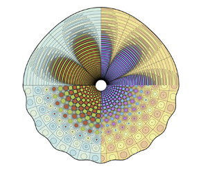
  $0$ to infinity. Only the 2-D filamentation perturbations of this form (no axial non-uniformity) are scale free, thereby enabling separation of variables in our perturbation equations for a cylindrical geometry (see sketch in figure 3). Regardless of the configuration, spherical or cylindrical, the stability analysis is done for one Fourier–Legendre mode at a time, so we omit the mode-number subscript $\sigma _{l,m}=\sigma$ for simplicity. The oscillation frequency will be dictated by the value of $\sigma _{I}$ while the real part will determine if the shock is stable ( $\sigma _{R}\leq 0$) or unstable ( $\sigma _{R}>0$).

Figure 3. Sketch of the cylindrical perturbed shock moving through the non-uniform upstream flow. Representation for the cylindrical geometry with  $m=10$.
Likewise, the perturbed density, pressure and radial velocity functions are written as
 \begin{gather} \bar{\rho}=\frac{\delta \rho}{\rho_s}=\frac{\rho(\theta,\varphi,\eta,t)-\rho_s}{\rho_s} = \epsilon \sum_{l,m}\left(\frac{t}{t_0}\right)^\sigma G(\eta)Y_l^m(\theta,\varphi), \end{gather}
 \begin{gather}\bar{p}=\frac{\delta p}{\rho_s c_s^2}=\frac{p(\theta,\varphi,\eta,t)-p_s}{\rho_s c_s^2} = \epsilon \sum_{l,m}\left(\frac{t}{t_0}\right)^\sigma P(\eta)Y_l^m(\theta,\varphi), \end{gather}
 \begin{gather}\bar{v}_r=\frac{\delta v_r}{ c_s}=\frac{v_r(\theta,\varphi,\eta,t)}{c_s} =\epsilon \sum_{l,m}\left(\frac{t}{t_0}\right)^\sigma V(\eta)Y_l^m(\theta,\varphi), \end{gather}
where  $G(\eta ), P(\eta )$ and $V(\eta )$ are the corresponding eigenfunctions that depend on the self-similar variable conveniently constructed with the speed of sound in the compressed gas
 \begin{equation} \eta = \frac{r}{c_s t} = {\mathcal{M}}_2 \frac{\xi}{\xi_s}.\end{equation}
 The components of transverse velocity perturbations  $\delta \boldsymbol {v}_\perp = \delta v_\theta \boldsymbol {e}_{\theta }+\delta v_\varphi \boldsymbol {e}_{\varphi }$ are gathered together with the transverse divergence function
 \begin{equation} \bar{d}=\frac{r\nabla_\perp\boldsymbol{\cdot} \delta \boldsymbol{v}_\perp(\theta,\varphi,\eta,t)}{c_s} =\epsilon \sum_{l,m}\left(\frac{t}{t_0}\right)^\sigma D(\eta)Y_l^m(\theta,\varphi),\end{equation}
that involves the eigenfunction  $D(\eta )$.
The inclusion of the perturbed variables (2.13)–(2.17) into the Euler equations (2.1)–(2.3) yields
 \begin{gather} \left(\sigma-\eta \frac{\textrm{d}}{\textrm{d} \eta}\right)G + \frac{\textrm{d}V}{\textrm{d} \eta} + \frac{(\nu-1)V}{\eta}+\frac{D}{\eta}=0, \end{gather}
 \begin{gather}\left(\sigma-\eta \frac{\textrm{d}}{\textrm{d} \eta}\right)V+\frac{\textrm{d}P}{\textrm{d} \eta}=0, \end{gather}
 \begin{gather}\left(\sigma-\eta \frac{\textrm{d}}{\textrm{d} \eta}\right)D-j(j+\nu-2)\frac{P}{\eta}=0, \end{gather}
 \begin{gather}\left(\sigma-\eta \frac{\textrm{d}}{\textrm{d} \eta}\right)(G- P)=0, \end{gather}
now a system of ordinary differential equations that only involve geometrical parameters  $\nu$ and $j$. In writing the conservation of transverse momentum (2.20) we have made use of the identity $r^2\nabla _\perp ^2\bar {p}=-j(j+\nu -2)\bar {p}$. Note that the main mode number $j\geq 0$ is used to unify the notation for both cylindrical and spherical geometries. The former is given by $\nu =2$ and $j=m$ and the latter is represented by $\nu =3$ and $j=l$. This can be done since $r^2\nabla _\perp ^2\bar {p}=-l(l+1)\bar {p}$ in spherical geometry, thereby indicating that the perturbation growth does not depend on the azimuthal mode number $m$, but on the polar mode number $l=j$.
Simple manipulation of (2.18)–(2.21) yields
 \begin{align} (\eta^2-1)\frac{\textrm{d}^2P}{\textrm{d} \eta^2} -2\left[\eta(\sigma-1)+\frac{\nu-1}{2\eta}\right] \frac{\textrm{d}P}{\textrm{d} \eta} + \left[\sigma(\sigma-1)+\frac{j(j+\nu-2)}{\eta^2}\right] P=0,\end{align}
as the ordinary differential equation that describes the acoustic eigenfunction. The general solution can be written as a linear combination of two Gauss hypergeometric functions  ${}_2 F_1$, but imposing the solution to be regular at the centre for any time, at $\eta =0$, leaves
 \begin{equation} P(\eta) = C_{ac} \eta^j {}_2F_1\left(\frac{j-\sigma}{2},\frac{j+1- \sigma}{2};j+\frac{\nu}{2};\eta^2\right),\end{equation}
where  $C_{ac}$ is the acoustic amplitude to be determined with the aid of the boundary conditions at the shock. Density perturbations eigenfunction
 \begin{equation} G(\eta) = C_{en} \eta^\sigma+ C_{ac} \eta^j {}_2 F_1\left(\frac{j-\sigma}{2},\frac{j+1-\sigma}{2};j+\frac{\nu}{2};\eta^2\right)\end{equation}
is obtained by direct integration of (2.21). The first term on the right-hand side includes the constant  $C_{en}$ and it corresponds to the entropic contribution of the density perturbations. The eigenfunction for the velocity perturbations is also split into curl-free acoustic and divergence-free rotational contributions. The former is obtained by calculating the sonic velocity potential $\delta \boldsymbol {v}=\boldsymbol {\nabla } \phi$,
 \begin{equation} \phi=\epsilon c_s^2 t_0\sum_{l,m}\left(\frac{t}{t_0}\right)^{\sigma+1} \varPhi(\eta)Y_l^m(\theta,\varphi), \end{equation}
that, in terms of the corresponding eigenfunction, obeys
 \begin{equation} \eta\frac{\textrm{d}\varPhi}{\textrm{d}\eta}+(\sigma +1) \varPhi=P(\eta), \end{equation}
which gives
 \begin{equation} \varPhi(\eta)={C_{ac}}\frac{\eta^j }{j-1-\sigma} {}_2 F_1\left(\frac{j-\sigma}{2},\frac{j-1-\sigma}{2};j+\frac{\nu}{2}; \eta^2\right) \end{equation}
upon integration and setting the arbitrary constant to be zero. Note the denominator  $j-1-\sigma$ in the term accompanying the hypergeometric function, which states that the acoustic contribution becomes singular for $\sigma =j-1$, which is real and positive.
The rotational contribution is obtained from the divergence-free condition that states that the amplitude of the radial-rotational velocity perturbations must be  $j(j+\nu -2)/(\sigma +\nu -1)$ times the transverse-rotational velocity amplitude. In sum, the eigenfunction of the radial velocity field includes the rotational and acoustic contributions in the form
 \begin{align} V(\eta) &= C_{ro} j(j+\nu-2)\eta^\sigma+C_{ac} \eta^{j-1} \left[{}_2 F_1\left(\frac{j-\sigma}{2},\frac{j+1-\sigma}{2};j+\frac{\nu}{2};\eta^2\right)\right. \nonumber\\ & \quad + \frac{\sigma+1}{j-1-\sigma}\left.{}_2 F_1\left(\frac{j-\sigma}{2},\frac{j-1-\sigma}{2};j+\frac{\nu}{2};\eta^2\right)\right], \end{align}
while that corresponding to the transverse divergence eigenfunction reads as
 \begin{align} D(\eta) &={-}C_{ro}\ j(j+\nu-2)(\sigma+\nu-1)\eta^\sigma \nonumber\\ &\quad - C_{ac} \eta^{j-1}\frac{j(j+\nu-2)}{j-1-\sigma}{}_2 F_1\left(\frac{j-\sigma}{2},\frac{j-1-\sigma}{2};j+\frac{\nu}{2};\eta^2\right). \end{align}
 They include the constant  $C_{ro}$ in the rotational contribution along with the term $j(j+\nu -2)$ multiplying the function $\eta ^\sigma$. It dictates that the case $j=0$ renders no vortical perturbation downstream as the shock shape remains cylindrical/spherical regardless of its perturbed position. The three complex constants, $C_{ac}, C_{en}$ and $C_{ro}$, along with the complex eigenvalue $\sigma$ are determined with use made of the linearized RH equations at the shock position $\eta = v_s/c_s={\mathcal {M}}_2$.
The linearized mass, radial momentum and energy conservation equations across the shock (the latest expressed through the perturbation of the RH curve) are
 \begin{gather} \frac{{\mathcal{R}}-1}{{\mathcal{R}}}\frac{\delta v_s}{v_s} = \bar{\rho}_{1s}-\frac{\bar{v}_{1s}}{{\mathcal{R}}} - \bar{\rho}_s+\frac{\bar{v}_{s}}{{\mathcal{M}}_2}, \end{gather}
 \begin{gather}\frac{\bar{p}_s}{{\mathcal{M}}_2^2}= \frac{\bar{p}_{1s}}{{\mathcal{R}}}+ {\mathcal{R}}\bar{\rho}_{1s}-2\bar{v}_{1s}+\frac{2\bar{v}_{s}}{{\mathcal{M}}_2} - \bar{\rho}_s, \end{gather}
 \begin{gather}\bar{\rho}_s ={-}\frac{h}{{\mathcal{M}}_2^2}\bar{p}_s + \frac{{\mathcal{M}}_1^2-1}{{\mathcal{M}}_1^2}{\mathcal{R}}^2h_1 \bar{\rho}_{1s}, \end{gather}
respectively, where  $h$ is the DK parameter defined in (1.1) and
 \begin{equation} h_1= \frac{h}{{\mathcal{M}}_1^2-1}\left[\left.\frac{1}{c_{s1}^2}\frac{\partial p_s}{\partial \rho_{1s}}\right|_{\rho_2,p_{1s}} + \left.\frac{\partial p_s}{\partial p_{1s}}\right|_{\rho_2,\rho_{1s}}\right], \end{equation}
accounts for the influence in the post-shock values due to the non-uniform pre-shock variables. For an ideal-gas EoS, they read as
 \begin{equation} h={-}\frac{1}{{\mathcal{M}}_1^2} \quad \text{and} \quad h_1= \frac{(\gamma-1)({\mathcal{M}}_1^2-1)}{(\gamma+1){\mathcal{M}}_1^2},\end{equation}
while the corresponding expressions for a vdW gas and a three-terms EoS for metals are provided in Appendix A.
As sketched in figure 3, the perturbed shock front encounters upstream variances along the radial coordinate as a consequence of the converging flow mass accumulation, which results in non-uniform density, pressure and velocity fields. The amplitudes of these perturbations depend on the local shock distortion range, which can be normalized with unity mode amplitude  $\zeta _{l,m}=1$ for any given values of $l$ and/or $m$ (Fourier mode). Since $\delta r_s=r_s-v_s t\sim \epsilon v_s t$ is given in (2.12), the local velocity perturbation by the shock distortion reads as
 \begin{equation} \frac{\delta v_s}{v_s}=\frac{1}{v_s}\frac{\partial r_s}{\partial t}= \epsilon (\sigma+1)\left(\frac{t}{t_0}\right)^\sigma Y_l^m(\theta,\varphi),\end{equation}
and the corresponding upstream dimensionless perturbations, related by the isentropic compression of the order of  $\epsilon$, are
 \begin{equation} \bar{\rho}_{1s}= \frac{{\mathcal{M}}_1^2}{{\mathcal{R}}^2}\bar{p}_{1s} = \frac{{\mathcal{M}}_1^2}{{\mathcal{R}}}\bar{v}_{1s} ={-}\epsilon (\nu-1)\frac{{\mathcal{M}}_1^2({\mathcal{R}}-1)}{{\mathcal{R}}({\mathcal{M}}_1^2-1)}\left(\frac{t}{t_0}\right)^\sigma Y_l^m(\theta,\varphi),\end{equation}
where  $\bar {\rho }_{1s}=\delta \rho _{1}/\rho _{1s}, \bar {v}_{1s}=\delta v_{1}/v_s$, and $\bar {p}_{1s}=\delta p_{1}/(\rho _{1s}v_s^2)$.
In terms of the eigenfunctions, linear combination of (2.30)–(2.32), along with the substitution of the compressed gas perturbation functions (2.13)–(2.15) and the upstream perturbation by the shock distortion (2.35) and (2.36) renders
 \begin{gather} \frac{{\mathcal{R}}}{{\mathcal{M}}_2^2({\mathcal{R}}-1)}P_s= \frac{2(\sigma+\nu)-{\mathcal{R}}(\nu-1)(1+h_1 )}{1+h}, \end{gather}
 \begin{gather}\frac{{\mathcal{R}}}{{\mathcal{R}}-1}G_s={-}\frac{2h(\sigma+\nu)-{\mathcal{R}}(\nu-1)(h -h_1 )}{1+h}, \end{gather}
 \begin{gather}\frac{{\mathcal{R}}}{{\mathcal{M}}_2({\mathcal{R}}-1)}V_s= \frac{(1-h)(\sigma+\nu)+{\mathcal{R}}(\nu-1)(h -h_1)}{1+h}, \end{gather}
for the values of pressure, density and velocity eigenfunctions at the shock (identified with the subscript  $s$), respectively. Unlike the 1-D problem, the distorted shock involves an additional unknown related to the transverse perturbations. Then, the fourth boundary condition at the shock completes upon integration of the transverse momentum conservation equation that reduces to
 \begin{equation} \frac{1}{{\mathcal{M}}_2({\mathcal{R}}-1)}D_s=j(j+\nu-2),\end{equation}
in terms of the eigenfunction  $D_s$. Equations (2.37)–(2.40) provide four boundary conditions to be employed in determining the complex values of $C_{ac}, C_{en}, C_{ro}$ and $\sigma$, with use made of (2.23)–(2.29). Note that they reduce to (20)–(23) in Velikovich et al. (Reference Velikovich, Murakami, Taylor, Giuliani, Zalesak and Iwamoto2016) for an ideal gas in the strong-shock limit ${\mathcal {M}}_1\gg 1$, whose governing parameters read as ${\mathcal {R}}=h_1^{-1}={\mathcal {M}}_2^{-2}-1=(\gamma +1)/(\gamma -1)$ and $h=0$.
By equating the eigenfunctions (2.23), (2.24), (2.28) and (2.29) evaluated at  $\eta ={\mathcal {M}}_2$ with the shock boundary conditions (2.37)–(2.40), respectively, the dispersion relationship that determines the eigenvalue $\sigma$ is found, namely
 \begin{align} &\{(\sigma+\nu-1) [{\mathcal{R}} (\nu-1)-\sigma-\nu ] + {\mathcal{R}} j (j+\nu-2)\}(1+h)F_{1s}^+ \nonumber\\ &\quad +[2(\sigma+\nu)-{\mathcal{R}}(\nu-1)(1 +h_1 )](\sigma+\nu+j-1)F_{1s}^-{=}0, \end{align}
where the functions  $F_{1s}^+$ and $F_{1s}^-$, defined conjointly as
 \begin{equation} F_{1s}^{{\pm}}= {}_2 F_1\left(\frac{j-\sigma}{2},\frac{j\pm1-\sigma}{2};j+\frac{\nu}{2};\eta^2={\mathcal{M}}_2^2\right), \end{equation}
refer to the Gauss hypergeometric functions evaluated at the shock front.
The dispersion equation (2.41) is a spherical/cylindrical counterpart of the DK dispersion equation for an isolated planar shock, (90.10) of Landau & Lifshitz (Reference Landau and Lifshitz1987). In planar geometry it is impossible to derive a dispersion equation that takes a piston into account. This is why the shock-front stability analysis had either to be done heuristically (Fowles & Swan Reference Fowles and Swan1973; Kuznetsov Reference Kuznetsov1984) or use much more complicated mathematics to solve the initial-value problem (Wouchuk & Cavada Reference Wouchuk and Cavada2004; Bates Reference Bates2015). By contrast, our dispersion equation (2.41) accounts for the piston-like represented by the centre or axis of symmetry. For a given geometric parameter  $\nu$ and four shock parameters, ${\mathcal {M}}_2, {\mathcal {R}}, h$ and $h_1$, the expanding shock front is unstable if for any angular mode number $j$ there is an eigenvalue with $\sigma _{R}>0$. Note that all the parameters entering (2.41) are real and the left-hand side of this equation is an analytic function of the complex parameter $\sigma$, thereby providing pairs of physically equivalent complex-conjugate eigenvalues, of which we only show those with non-negative $\sigma _{I}$.
The dispersion relationship (2.41) does not admit an analytical solution except for some limiting cases. For example, benefiting from the simplification of the hypergeometric function for the lowest mode  $j=0$ in spherical geometry $\nu =3$,
 \begin{equation} F_{1s}^{{\pm}}(j=0,\nu=3)=\frac{(1+{\mathcal{M}}_2)^{\sigma+3/2 \mp 1/2}-(1-{\mathcal{M}}_2)^{\sigma+3/2 \mp 1/2}}{2(\sigma+3/2 \mp 1/2){\mathcal{M}}_2},\end{equation}
the dispersion relationship can be written in explicit form
 \begin{align} &(\sigma+2)[2{\mathcal{R}}-(\sigma+3) ] (1+h)(\mathscr{D}_s^{\sigma+1}-1) \nonumber\\ &\quad +2(\sigma+1)[(\sigma+3)-{\mathcal{R}}(1 +h_1 )](\mathscr{D}_s^{\sigma+2}-1)(1-{\mathcal{M}}_2)=0, \end{align}
provided that  $\sigma \neq -2$ and $\sigma \neq -1$, since writing (2.44) involves the multiplication of the two terms by $(\sigma +2)(\sigma +1)$. Equation (2.44), which includes the Doppler shift factor
 \begin{equation} \mathscr{D}_s =\frac{1+{\mathcal{M}}_2}{1-{\mathcal{M}}_2}>1,\end{equation}
associated with the coupling with the centre of symmetry, provides the values of  $\sigma$ for a purely radial perturbation of the shock front: it assumes that the shock is slightly displaced from its corresponding equilibrium position given by the base-flow theory presented before.
For an ideal-gas EoS, the four parameters that describe the shock properties in the dispersion relationship (2.41) can be reduced to two: typically the shock Mach number  ${\mathcal {M}}_1$ and the adiabatic index $\gamma$, although the former can be substituted by any other jump property. Then, with use made of (A 9) and (2.34a,b), the corresponding dispersion relationship for a finite-strength shock reads as
 \begin{align} &\{(\sigma+\nu-1)[(\gamma+1){\mathcal{M}}_1^2(\sigma+2\nu-1-\gamma-\sigma\gamma)-2(\sigma+\nu)]\nonumber\\ &\quad +j(j+\nu-2)(\gamma+1) {\mathcal{M}}_1^2\}(1-{\mathcal{M}}_1^{{-}2})F_{1s}^+{+}[1-\gamma+3\nu+4\sigma+\nu\gamma \nonumber\\ &\quad -2{\mathcal{M}}_1^2(\sigma+\nu-\sigma\gamma-\gamma)](\sigma+\nu+j-1)F_{1s}^{-} = 0, \end{align}
which only depends on  ${\mathcal {M}}_1$ and $\gamma$ for a given perturbation mode number $j$ and geometry parameter $\nu$. This expression can be further reduced in the strong-shock limit, ${\mathcal {M}}_1\gg 1$, to yield (29) in Velikovich et al. (Reference Velikovich, Murakami, Taylor, Giuliani, Zalesak and Iwamoto2016). In the weak-shock limit, ${\mathcal {M}}_1-1\ll 1$, the function $h+1$ approaches zero thereby cancelling out the term proportional to $h+1$ in (2.41), or the term proportional to $(1-{\mathcal {M}}_1^{-2})$ in (2.46), when $\sigma$ remains finite. However, high-order modes still contribute so long as $\sigma ^2({\mathcal {M}}_1-1)\sim 1$ or higher.
3. Results
3.1. The eigenvalues
The dispersion equation (2.41) renders an infinite number of eigenmodes for each perturbation mode number  $j$. They are numbered by $n=1, 2,\ldots ,$ in the order of increasing $\sigma _{I}$; $n$ is called the radial mode number. The distinction between the radial $n$ and transverse $j$ mode numbers can be used to study some distinguished limits of the eigenvalues pool, such as the limits $n\gg j$ and $j\gg n$ addressed below. While the former corresponds to radial acoustic perturbations, the latter is representative of planar shocks, where transverse perturbations dominate.
High-order modes  $n\gg j$ can be also treated analytically with use made of the quadratic transformation of the Gauss hypergeometric in the corresponding high-frequency limit to give
 \begin{align} F_{1s}^{{\pm}}&\underset{n\gg j}{=} (1+{\mathcal{M}}_2)^{\sigma-j} \frac{\varGamma(2j+\nu-1)}{\varGamma[j+(\nu-1)/2]} \left[\frac{1+{\mathcal{M}}_2}{2{\mathcal{M}}_2(j-\sigma)}\right]^{j+(\nu-1)/2} \nonumber\\ &\quad \times [(-\textrm{i})^{2j+\nu-1}+\mathscr{D}_s^{\sigma +\nu/2\mp 1/2}]+O(j/|\sigma|) \end{align}
for the two hypergeometric functions defined in (2.42), where  $\varGamma$ is the gamma function and $\mathscr {D}_s$ is the Doppler shift factor defined in (2.45). Upon substitution in (2.41), the corresponding dispersion relationship for high-order modes reads as
 \begin{equation} (1+2{\mathcal{M}}_2-h)(-\textrm{i})^{2j+\nu-1} + (1-2{\mathcal{M}}_2-h)\mathscr{D}_s^{-\sigma -(\nu-1)/2}=0, \end{equation}
provided that only the dominant contribution  $O(\sigma ^2)$ is retained in (2.41). The poles in (3.2) satisfy
 \begin{gather} \sigma_{R}^{(n\gg j)}\sim{-} \frac{\nu-1}{2} + \frac{\ln |\mathscr{R}_s|}{\ln \mathscr{D}_s}, \end{gather}
 \begin{gather}\sigma_{I}^{(n\gg j)}\sim \frac{2{\rm \pi} n}{\ln \mathscr{D}_s}+O(1), \end{gather}
for the real and imaginary components, respectively. Here
 \begin{equation} \mathscr{R}_s = \frac{2{\mathcal{M}}_2 -1+ h}{2{\mathcal{M}}_2+1-h},\end{equation}
stands for the reflection coefficient for an acoustic wave normally incident on the shock front from behind (we refer to Rutkevich & Mond (Reference Rutkevich and Mond1992) for its extension to fast magnetoacoustic waves hitting the shock). For  $1< h<1+2{\mathcal {M}}_2$, we have $\mathscr {R}_s>1$, so acoustic waves are amplified upon reflection from the shock front, indicating instability for planar geometry, in agreement with Fowles & Swan (Reference Fowles and Swan1973), Kuznetsov (Reference Kuznetsov1984).
When the radial mode number is sufficiently large, the value of  $\sigma _{R}$ approaches that predicted in (3.3a) and the frequency increase between two successive radial mode numbers becomes constant with the value predicted in (3.3b). In this limit $n\gg j$, acoustic waves reverberate almost normally to the shock front, as illustrated below in figures 10 and 11. The relevant length scale, $\sim v_s t/n$, is much smaller than those associated with the pre-shock non-uniformity and the angular mode number, $\sim v_s t$ and $\sim v_s t/j$, respectively, which explains why parameters $h_1$ and $j$ do not enter (3.3a) and (3.3b). Although (2.41) does not apply to planar geometry, $\nu =1$, the asymptotic formulae (3.3a) and (3.3b) are valid in this case, too. They describe an acoustic wave reverberating between the shock front and the piston at the speed of sound, $c_s$, whereas the shock front moves away from the piston at velocity $v_s$. Its back-and-forth cycles increase in duration as powers of the Doppler shift factor: $t_1, \mathscr {D}_s t_1, \mathscr {D}_s^2 t_1$,…, cf. figure 3 of Fowles & Swan (Reference Fowles and Swan1973). Assuming the reflection coefficient from the piston to be unity, in planar geometry each cycle multiplies the acoustic wave's amplitude by the shock reflection coefficient: $1, \mathscr {R}_s, \mathscr {R}_s^2,\ldots$. The amplitude thus varies as a complex power of time, the real part of the power index for $\nu =1$ being given by the second term on the right-hand side of (3.3a). The first term, negative for $\nu =2$ and $3$, describes the attenuation of diverging acoustic waves, as explained in Velikovich et al. (Reference Velikovich, Murakami, Taylor, Giuliani, Zalesak and Iwamoto2016). The stabilizing effect of divergence is obviously stronger for spherical expansion.
Figure 4 shows the eigenvalues for  $\nu =2$ (boxes) and $\nu =3$ (circles), for shocks with ${\mathcal {R}}=3$ with low-mode numbers $j=0, 1, 2$ and $3$ in three different EoS (ideal gas for air, vdW and aluminum). In these conditions, none of the cases considered renders unstable oscillations, although the shock moving in a vdW EoS with the conditions that render SAE in planar shocks ( $\gamma =31/30, \alpha _1=1/2$ and $\beta _1=1/9$), see Bates & Montgomery (Reference Bates and Montgomery2000), has the largest value of $\sigma _{R}$ with $\sigma _{I}\neq 0$. This complex eigenvalue, which seems to correspond to the lowest $n$ and the largest $j$, is the dominant contribution to the decaying oscillations of the perturbed shock.

Figure 4. Eigenvalues for  $\nu =2$ (boxes) and $\nu =3$ (circles), for shocks with ${\mathcal {R}}=3$ with low-mode numbers $j=0, 1, 2$ and $3$ in three different EoS (ideal gas for air, vdW and aluminum).
When  $n\gg j$, the poles align along the asymptotic values predicted in (3.3a), represented with a vertical grey dashed lines in figure 4. Although none of the examples yields instability, it is interesting to evaluate the condition on the DK parameter $h$ that gives $\sigma _{R}^{(n\gg j)}>0$, namely
 \begin{equation} h>h_m=1+2{\mathcal{M}}_2\frac{\mathscr{D}_s^{({\nu-1})/{2}}-1}{\mathscr{D}_s^{({\nu-1})/{2}}+1},\end{equation}
which can be applied to  $\nu =1, 2$ and $3$. As $h$ increases from the value in (3.5) to $h=1+2{\mathcal {M}}_2$ (the value that makes singular the reflection coefficient $\mathscr {R}_s$), the corresponding power index $\sigma _{R}$ given by (3.3a) increases from zero to infinity. However, the instability threshold for cylindrical and spherical shocks when $n\gg j$ occurs before because $h_m<1+2{\mathcal {M}}_2$. Note, however, that it gives sufficient rather than necessary instability conditions. The modes with large $n\gg j$ are not necessarily the most unstable. The instability is quite possible when the right-hand side of (3.3a) is negative. For example, for a vdW EoS, poles with low radial mode number in figure 4 lie on the right of the vertical asymptotic line, and the largest value corresponds to the largest perturbation mode number $j=3$.
In order to evaluate if the increase of the transverse mode number  $j$ may eventually lead to instability, the eigenvalues are now computed for large $j\gg n$ in figure 5 for the same EoS (ideal gas for air, vdW and aluminum) and shock conditions as those used in figure 4. In particular, the eigenvalues for $j=15, 50, 150$ and $300$ are plotted in the complex plane, with the vertical axis being normalized with respect to the angular mode number, $\sigma _{I}/j$, to show all spectra on the same scale. For each $j$, figure 5 shows several complex eigenvalues corresponding to low radial mode numbers $n=1$ to $8$. As $j$ increases, the poles align along the horizontal asymptotic value
 \begin{equation} \lim_{j\rightarrow\infty}\frac{\sigma_{I}}{j}= \sqrt{{\mathcal{M}}_2^{{-}2}-1},\end{equation}
either on the negative half-plane  $\sigma _{R}<0$ (for the ideal gas and the aluminum EoS) or, eventually, on the positive half-plane $\sigma _{R}>0$ (for the vdW EoS). The value in (3.6) is readily obtained by knowing that the shock front is effectively planar in the short-wavelength limit $j\rightarrow \infty$. Then, the oscillation frequency $\omega _s$ of shock-front ripples is related to the transverse wavenumber $k$ by $\omega _s=k c_s (1-{\mathcal {M}}_2^2)^{1/2}$ (Zaidel’ Reference Zaidel’1960). Substituting $\omega _s=\sigma _{I}/t$ and $k=j/(v_s t)$ for the frequency and wavenumber, respectively, gives the value (3.6), represented in grey dashed lines in figure 5.

Figure 5. Eigenvalues for  $\nu =2$ (boxes) and $\nu =3$ (circles), for shocks with ${\mathcal {R}}=3$ with low-mode numbers $j=15, 50, 150$ and $300$ in three different EoS (ideal gas for air, vdW and aluminum).
Two distinguished scenarios are observed in figure 5. For the ideal gas and the aluminum three-terms EoS, the shape of the poles plotted on the  $\{\sigma _{R}$, $\sigma _{I}/j\}$ plane is very similar, with all the eigenvalues being on the negative half-plane $\sigma _{R}<0$, i.e. stable conditions. There exist, however, differences in the dominant poles as $j$ increases. The short-wavelength limit is better analysed in figure 6 that shows the value of $\sigma _{R}$ vs mode number $j$ for low radial mode numbers with the same conditions as those in figures 5(a) and 5(c) : a shock with ${\mathcal {R}}=3$ moving through an ideal gas with $\gamma =7/5$(a) and aluminum modelled with the three-terms EoS (b). For air, it is found that the dominant contribution is the high-mode radial eigenvalue, that renders $\sigma _{R}^{(n\gg j)}=-2.9578$ in cylindrical geometry, a value that shifts $-0.5$ units in the spherical case. For $j\gg n$, the maximum value for $\sigma _{R}$ approaches $\sim -4.27$ for $\nu =2$ ( $-0.5$ units for $\nu =3$). It indicates that, regardless of the value of $j$, radial perturbations decay slower and thus they dominate in the long-time regime. Computations for aluminum, displayed in figure 6(b) show that eigenvalues with low radial mode number dominate with respect to high radial mode number $\sigma _{R}^{(n\gg j)}$. Unlike the unstable case of vdW displayed in figure 5(b), the dominant low- $n$ eigenmode does not correspond to the lowest $n=1$, but it rather shifts up in one unity when increasing the mode number $j$. For example, $\sigma _{R}^{(n\gg j)}=-3.48442$ for cylindrical geometry ( $-0.5$ units in spherical geometry) but the alternating dominant mode number approaches $\sim -3.45$ ( $-0.5$ units for $\nu =3$) when $j\gg n$, which is slightly larger than that predicted for $n\gg j$. That makes the radial mode number $n$ a relevant parameter in describing the perturbations decay rate even for short transverse wavelengths, so that $j\gg n$ is not strictly applicable. Regardless of the case, the decay rate is not a universal power law, as occurs for planar isolated shocks, but it depends on the shock properties, flow geometry $\nu$ and perturbation mode number $j$.
$j$.

Figure 6. Decay power law  $\sigma _{R}<0$ vs mode number $j$ for $n=1$– $8$ in cylindrical (orange) and spherical (blue) geometries. Shock with ${\mathcal {R}}=3$ moving in an ideal gas with $\gamma =7/5$ (a) and cold aluminum (b).
For the case of the vdW EoS, figure 5(b) displays a very different pattern. Computations made for  $\gamma =31/30, \alpha _1=1/2, \beta _1=1/9$ and ${\mathcal {R}}=3$, conditions that are known to exhibit SAE in planar isolated shocks (Bates & Montgomery Reference Bates and Montgomery2000), reveal that the increase of the mode number $j$ gives higher values of $\sigma _{R}$, with the lowest radial mode $n=1$ being the largest for each value of $j$. If $j$ is sufficiently large, the leading pole may cross the stability threshold $\sigma _{R}=0$, which is found to occur for $j=300$ in cylindrical geometry (leading box), but it does not happen in spherical geometry (leading circle). Numerical evaluation of these two cases places the onset of instability at $j=258$ for $\nu =2$ and $j=364$ for $\nu =3$. The study of the stability limits is extended in the next subsection.
3.2. The stability limits
For a given set of the shock parameters, spherical or cylindrical geometry, and any given finite value of  $j$, we find a distinct value of the parameter $h$ that determines the shock ripple behaviour, $h_{st}$, corresponding to $\sigma _{R}=0$. At $h=h_{st}$, the oscillating and growing shock ripples maintain a constant amplitude relative to the shock radius. Above this threshold, at $h>h_{st}$, the shock ripple amplitude grows faster than the shock front expands, indicating instability. Then, downstream pressure and density perturbations, which scale with the shock distortion rate, grow both absolutely and relatively.
Usually, the most unstable eigenvalue has the lowest radial mode number  $n$. The instability threshold corresponds to a purely imaginary eigenvalue: $\sigma _{R}=0$ and $\sigma =\textrm {i} s$, where $s$ is real and positive. To determine its location, we solve (2.41) for $h$ and substitute $\sigma =\textrm {i} s$ into the result, arriving at
 \begin{equation} \hat{h}(s)={-}1 -\left.\frac{[2(\textrm{i} s+\nu)-{\mathcal{R}}(\nu-1) (1 + h_1 )](\textrm{i} s+\nu+j-1)}{(\textrm{i} s+\nu-1) [{\mathcal{R}} (\nu-1)-\textrm{i} s-\nu ] + {\mathcal{R}} j (j+\nu-2)} \frac{F_{1s}^-}{F_{1s}^+}\right|_{\sigma=\textrm{i} s}.\end{equation}
 For an arbitrary value of  $s$, the right-hand side of (3.7) is complex, implying that $\sigma =\textrm {i} s$ is not a physically meaningful eigenvalue because $h$ must be real. However, for given values of ${\mathcal {M}}_2, {\mathcal {R}}, h_1, \nu$ and $j$, the equation $\textrm {Im}[\hat {h}(s)]=0$ for (3.7) has an infinite number of solutions $s^{(1)}, s^{(2)},\ldots , s^{(n)},\ldots$ that are actual eigenvalues. They correspond to conditions when the eigenmodes with radial numbers $n=1, 2,\ldots$ cross the lines $\sigma _{R}=0$ as $h$ increases. Substituting them into (3.7) we find the corresponding real values of $h=h^{(1)}, h^{(2)},\ldots , h^{(n)},\ldots$, associated with neutral oscillations. The lowest of these values found in the range between $-1$ and $h_m$ defined in (3.5) is the instability threshold denoted by $h_{st}({\mathcal {M}}_2,{\mathcal {M}},h_1,\nu ,j)$.
This is better illustrated in figure 7, where the real and imaginary parts of  $\hat {h}$ are plotted as a function of the frequency $s$ for $j=4$ (a) and $j=300$ (b), with the conditions used in figure 5(b) for a cylindrical shock moving in a vdW gas with $\gamma =31/30, \alpha _1=1/2$ and $\beta _1=1/9$. Shock jump properties are ${\mathcal {R}}=3, {\mathcal {M}}_2=0.7261$ and $h_1=0.0271$. Although $h$ is taken as an independent parameter in figure 7, the corresponding value at these conditions, $h=-0.51444$, is represented by the red line. The lowest value of $h^{(n)}$, that is found to be $h^{(1)}$, is the one defining the stability threshold $h_{st}$. In figure 7(a) it is observed that $h^{(1)}$ is larger than the actual value of $h=-0.51444, h< h_{st}$, which implies that the shock is stable for $j=4$ in these conditions. On the other hand, figure 7(b) shows the same parameters for $j=300$ and $h^{(1)}$ is found to be lower than $-0.51444$ (then $h>h_{st}$) that translates into unstable oscillations in agreement with figure 4(b). Note, however, that there exist more solutions for $\textrm {Im}[\hat {h}]=0$ (see grey circles in the left panel of figure 7) that are associated with a negative slope of the curve $\textrm {Im}[\hat {h}]$. However, since they render a family of solutions with higher values of $\textrm {Re}[\hat {h}]$ than that represented with blue circles, they are not meaningful in what refers to the search of the stability threshold.

Figure 7. Real and imaginary parts of  $\hat {h}$ for $j=4$ (a) and $j=300$ (b) as a function of the frequency $s$ for $\nu =2, {\mathcal {R}}=3, {\mathcal {M}}_2=0.7261$ and $h_1=0.0271$. The red line corresponds to the actual value $h=-0.51444$ for a vdW gas in these conditions.
To compare the value of  $h_{st}$ with the critical value for SAE given by (1.2), $h_c({\mathcal {M}}_2,{\mathcal {R}})$, we plot in figure 8 the difference $h_{st}({\mathcal {M}}_2,{\mathcal {R}},h_1,\nu ,j)-h_c({\mathcal {M}}_2,{\mathcal {R}})$ for a vdW gas (a) and for an ideal gas (b) as a function of the mode number $j$. Shock conditions are determined by ${\mathcal {R}}=3$, that renders ${\mathcal {M}}_2=0.72611, h=-0.5144$ $h_1=0.027076$ for a vdW gas with $\gamma =31/30, \alpha _1=1/2$ and $\beta _1=1/9$ (a), and ${\mathcal {M}}_2=0.542326, h=-0.2$ $h_1=0.1333$ for an ideal gas with $\gamma =7/5$ (b). The actual value of $h-h_c$, ( $0.025337$ for a vdW EoS and $-0.08889$ for air) is represented by red lines. The circles denote the condition $h_{st}-h_c=h-h_c$, which only occurs for the vdW gas at $j=258$ and $j=364$ for cylindrical and spherical geometries, respectively. For an ideal gas, the condition $h_{st}-h_c=h-h_c$ is never met, thereby indicating stability for any mode number $j$. For low and moderate angular mode numbers, the difference $h_{st}-h_c$ is significant, manifesting the stabilizing effect of expansion. But as $j$ increases into the high-mode range, $h_{st}-h_c$ tends to zero. The inset plotted therein demonstrates that they approach $h_c$ at $j\rightarrow \infty$ as a negative power of the mode number, $j^{-0.66}$. The demonstration of the limit
 \begin{equation} \lim_{j\rightarrow\infty}h_{st}({\mathcal{M}}_2,{\mathcal{R}},h_1,\nu,j)=h_c({\mathcal{M}}_2,{\mathcal{R}}),\end{equation}
is straightforward if we apply (3.6) in the limit  $j\rightarrow \infty$ to (3.7). On one side, the ratio of the Gauss hypergeometric functions in the short-wavelength limit approaches a constant complex value, namely
 \begin{equation} \left. \lim_{j\rightarrow\infty}\frac{F_{1s}^-}{F_{1s}^+}\right|_{\sigma=\textrm{i} j\sqrt{{\mathcal{M}}_2^{{-}2}-1}}=1-{\mathcal{M}}_2^2+\textrm{i} {\mathcal{M}}_2\sqrt{1-{\mathcal{M}}_2^2},\end{equation}
that does not depend on  $\nu$. On the other side, the factor multiplying the ratio of the Gauss hypergeometric functions gives
 \begin{equation} -\frac{2(1-{\mathcal{M}}_2^2-\textrm{i} {\mathcal{M}}_2\sqrt{1-{\mathcal{M}}_2^2})}{1+{\mathcal{M}}_2^2 ({\mathcal{R}}-1)}\end{equation}
in the short-wavelength limit  $j\rightarrow \infty$, which does not depend on $\nu$ nor $h_1$ either. Then, the product of (3.9) by (3.10) minus unity gives $h_c$, as specified in (3.8).

Figure 8. Functions  $h_{st}-h_c$ for a vdW gas with $\gamma =31/30, \alpha _1=1/2$ and $\beta _1=1/9$ (a) and an ideal gas with $\gamma =7/5$ (b) as a function of the mode number $j$ for ${\mathcal {R}}=3$. The red line corresponds to the actual value $h-h_c$ in these conditions.
Eigenmodes with high angular mode number  $j\rightarrow \infty$ and low radial mode number $n$ are the most unstable. For these modes, acoustic waves reverberating behind the shock front are nearly parallel to it as illustrated below in figures 10 and 11, in contrast with the high- $n$ modes described by (3.3a) and (3.3b). In the short-wavelength limit $j\rightarrow \infty$, the unperturbed shock front is almost planar, and the stabilizing effect of its spherical or cylindrical expansion vanishes. Similarly, the large-scale non-uniformity of the pre-shock flow is no longer relevant. This is why the expanding shock-front instability threshold tends to the planar-geometry critical SAE value (1.2). However, in contrast with the classic case of isolated planar shock, here we have ‘instability in a literal sense’ (Landau & Lifshitz Reference Landau and Lifshitz1987), all perturbation amplitudes exhibiting an oscillatory power-law growth with time, as illustrated in figure 1(b).
For the following vdW EoS parameters  $\gamma =31/30, \alpha _1=1/2$ and $\beta _1=1/9$, the DK instability condition $h>h_c$ is met within an interval of shock strengths corresponding to density compressions $2.2586<{\mathcal {R}}<3.1482$. As demonstrated in figure 8, this ensures instability of expanding shock waves for sufficiently high angular mode numbers $j$. Figure 9 shows the stability limits $h=h_{st}$ for spherical and cylindrical shocks. There exists a minimum value of $j=j_{min}$, below which the shock is stable for any shock compression ratio ${\mathcal {R}}$. For cylindrical and spherical geometries, we find $j_{min}=148$ and $213$, which occur at ${\mathcal {R}}\sim 2.8$. Figure 9 also presents the evolution of the perturbed shock radius (grey line) and shock distortion rate (black line) as a function of the dimensionless time $t/t_0$ for ${\mathcal {R}}=3$ and $\nu =2$ and two different mode numbers: $j=150$ and $j=300$, which render $\sigma _{R}=-0.565908$ (diamond symbol) and $\sigma _{R}=0.196671$ (star symbol), respectively.

Figure 9. (a) Plots of  $\sigma _{R}=0$ isocurves for cylindrical (blue) and spherical (brown) geometries. Gas properties of a vdW EoS with $\gamma =31/30, \alpha _1=1/2$ and $\beta _1=1/9$. (b,c) Evolution of the perturbed shock radius and shock velocity for ${\mathcal {R}}=3$ and $\nu =2$ and two different mode numbers $j=150$ and $j=300$ corresponding to $\sigma _{R}=-0.565908$ (diamond symbol) and $\sigma _{R}=0.196671$ (star symbol), respectively.
Note that the condition  $\sigma _{R}=-1$ distinguishes the case where the shock ripples oscillate at a constant amplitude, which gradually becomes smaller compared with the shock radius, then for $-1<\sigma _{R}<0$ (diamond symbol case), the amplitude of the shock grows absolutely because $\delta r_s \sim t^{\sigma +1}$, yet it decays relatively since $\delta r_s/(v_s t) \sim t^\sigma$. For $\sigma _{R}=0.196671>0$ (star symbol case), both relative and absolute shock ripple oscillations grow with time. Likewise, any case with $\sigma _{R}<-1$ will render relative and absolute decay of the shock oscillations.
3.3. The post-shock perturbation field
Once the eigenvalues are determined, the post-shock flow field can be defined with use made of the eigenfunctions in (2.23), (2.24), (2.28) and (2.29). For example, the amplitude associated with the acoustic eigenfunction is obtained with the aid of (2.37) in the equality  $P(\eta ={\mathcal {M}}_2)=P_s$ to give
 \begin{equation} C_{ac} = \frac{{\mathcal{R}}-1}{{\mathcal{R}}{\mathcal{M}}_2^{j-2}} \frac{2(\sigma+\nu)-{\mathcal{R}}(\nu-1)(1+h_1 )}{1+h }\frac{1}{F_{1s}^+}. \end{equation}
 According to (2.23), the eigenfunction for the acoustic contributions,  $P(\eta )$ for pressure, is finite everywhere and it can be used to represent the pressure field behind the shock. Figure 10(a) shows the spatial distribution of the acoustic field in two distinct cases. In panel (a) the perturbations for low-mode number $j=4$ and relatively high radial number $n=20$ are represented, while an opposite case is displayed in panel (c), corresponding to $j=20$ and $n=1$. Differences are clear: the former is dominated by radial disturbances and the latter by lateral perturbations. Note that this picture does not change qualitatively with time as it represents a standing sonic wave whose spatial distribution changes collectively to satisfy the corresponding pressure value at the shock front. This is better analysed on the right-hand side of figure 10, where the pressure field is represented along the radial coordinate $r/(v_st_0)$ at different times $t=t_0/2, t=t_0$ and $t=2t_0$. The grey curve corresponds to the history of pressure perturbations at the shock position $r=v_s t$ for $\varphi =0$. The associated pressure field downstream is stretched along the radial axis, with no change in the number of peaks and valleys, while the amplitude is accordingly modified by the value at the shock.

Figure 10. Analytic pressure field for dominantly radial perturbations  $n\gg j$ and dominantly transverse perturbations $j\gg n$ for a shock wave moving in a vdW gas.
The corresponding amplitudes for the entropic and rotational contributions to the density and velocity eigenfunctions can be derived with use made of  $G(\eta ={\mathcal {M}}_2)=G_s$ and $V(\eta ={\mathcal {M}}_2)=V_s$ or, equivalently, $D(\eta ={\mathcal {M}}_2)=D_s$, with the values at the shock being (2.38), (2.39) and (2.40), respectively. We arrive at
 \begin{equation} C_{en} ={-} \frac{ {\mathcal{R}}-1 }{{\mathcal{M}}_2^{\sigma}{\mathcal{R}}} \frac{2(\sigma+\nu)(h+{\mathcal{M}}_2^2)-{\mathcal{R}}(\nu-1)[h+{\mathcal{M}}_2^2-h_1(1-{\mathcal{M}}_2^2)]}{1+h},\end{equation}
and
 \begin{equation} C_{ro} ={-}\frac{{\mathcal{R}}-1}{(\sigma+\nu-1){\mathcal{M}}_2^{\sigma-1}}\left[1+\frac{2(\sigma+\nu)-{\mathcal{R}}(\nu-1)(1 +h_1)}{{\mathcal{R}} (1+h)(j-1-\sigma)}\frac{ F_{1s}^-}{ F_{1s}^+}\right],\end{equation}
respectively.
Entropic and rotational perturbations do not propagate through the shocked gas, they are localized in the fluid particles in absence of diffusive effects. Their contribution, proportional to  $(\eta \ t/t_0)^\sigma$, exclusively depends on the dimensionless radial position $r/(v_s t_0)$ and the polar $\theta$ and azimuthal $\varphi$ coordinates. For example, the entropic contribution of density perturbations reads as
 \begin{equation} \bar{\rho}^{en}(r,\theta,\varphi)= \epsilon \sum_{l,m}{\zeta_{l,m}}\left(\frac{r}{ v_s t_0}\right)^\sigma C_{en} Y_l^m(\theta,\varphi), \end{equation}
where both the factor  $C_{en}$ and the eigenvalue $\sigma$ are, in fact, functions of $l$ and $m$. Likewise, the rotational contribution of the velocity field is
 \begin{gather} \bar{v}_r^{ro}(r,\theta,\varphi)= \epsilon \sum_{l,m}{\zeta_{l,m}}j(j+\nu-2) \left(\frac{r}{ v_s t_0}\right)^\sigma C_{ro} Y_l^m(\theta,\varphi), \end{gather}
 \begin{gather}\bar{v}_\theta^{ro}(r,\theta,\varphi)= \epsilon \sum_{l,m}{\zeta_{l,m}}(\sigma+\nu-1) \left(\frac{r}{ v_s t_0}\right)^\sigma C_{ro}\frac{\textrm{d} P_l^m}{\textrm{d}\theta} \exp(\textrm{i} m \varphi), \end{gather}
 \begin{gather}\bar{v}_\varphi^{ro}(r,\theta,\varphi)= \epsilon \sum_{l,m}{\zeta_{l,m}}(\sigma+\nu-1)\left(\frac{r}{ v_s t_0}\right)^\sigma C_{ro}\frac{\textrm{i} m}{\sin \theta} Y_l^m(\theta,\varphi), \end{gather}
where  $P_l^m=P_l^m(\cos \theta )$ stands for the associated Legendre polynomial.
Associated with the rotational contribution is the dimensionless vorticity field
 \begin{equation}
\boldsymbol{\bar{\omega}}=\omega t_0= \begin{pmatrix}
\bar{\omega}_r\\ \bar{\omega}_\theta\\ \bar{\omega}_\varphi
\end{pmatrix} = \begin{pmatrix}
-\dfrac{1}{r\sin\theta}\dfrac{\partial
\bar{v}_\theta^{ro}}{\partial
\varphi}+\dfrac{1}{r}\dfrac{\partial
\bar{v}_\varphi^{ro}}{\partial
\theta}+\dfrac{\bar{v}_\varphi^{ro}}{r\tan \theta}\\
\dfrac{1}{r\sin\theta}\dfrac{\partial
\bar{v}_r^{ro}}{\partial \varphi}-\dfrac{\partial
\bar{v}_\varphi^{ro}}{\partial
r}-\dfrac{\bar{v}_\varphi^{ro}}{r}\\
-\dfrac{1}{r}\dfrac{\partial \bar{v}_r^{ro}}{\partial
\theta}+\dfrac{\partial \bar{v}_\theta^{ro}}{\partial
r}+\dfrac{\bar{v}_\theta^{ro}}{r} \end{pmatrix}
\end{equation}
\begin{equation}
\boldsymbol{\bar{\omega}}=\omega t_0= \begin{pmatrix}
\bar{\omega}_r\\ \bar{\omega}_\theta\\ \bar{\omega}_\varphi
\end{pmatrix} = \begin{pmatrix}
-\dfrac{1}{r\sin\theta}\dfrac{\partial
\bar{v}_\theta^{ro}}{\partial
\varphi}+\dfrac{1}{r}\dfrac{\partial
\bar{v}_\varphi^{ro}}{\partial
\theta}+\dfrac{\bar{v}_\varphi^{ro}}{r\tan \theta}\\
\dfrac{1}{r\sin\theta}\dfrac{\partial
\bar{v}_r^{ro}}{\partial \varphi}-\dfrac{\partial
\bar{v}_\varphi^{ro}}{\partial
r}-\dfrac{\bar{v}_\varphi^{ro}}{r}\\
-\dfrac{1}{r}\dfrac{\partial \bar{v}_r^{ro}}{\partial
\theta}+\dfrac{\partial \bar{v}_\theta^{ro}}{\partial
r}+\dfrac{\bar{v}_\theta^{ro}}{r} \end{pmatrix}
\end{equation}
that can be expressed in separated variables as
 \begin{equation} \boldsymbol{\bar{\omega}}=\epsilon\left(\frac{t}{t_0}\right)^{\sigma-1} \left[\varOmega_r(\eta)Y_l^m,\varOmega_\theta(\eta)\frac{\textrm{i} m}{\sin\theta}Y_l^m,\varOmega_\varphi(\eta) \frac{\textrm{d} P_l^m}{\textrm{d}\theta}\exp(\textrm{i} m \varphi)\right], \end{equation}
where  $\varOmega _r(\eta ), \varOmega _\theta (\eta )$ and $\varOmega _\varphi (\eta )$ are the corresponding eigenfunctions. It is immediate to see that $\varOmega _r=0$, since the shock conserves the vorticity component that points normal to the shock front, and $\varOmega _\theta (\eta )=-\varOmega _\varphi (\eta )= C_{ro} \eta ^{\sigma -1}(j-\sigma -1)(j+\sigma +\nu -1)$ because of the symmetry of the perturbations. Then, as occurred with the entropic and the rotational velocity fields, the vorticity function
 \begin{align} \boldsymbol{\bar{\omega}}(r,\theta,\varphi)= \epsilon \sum_{l,m}{\zeta_{l,m}}\left(\frac{r}{v_s t_0}\right)^{\sigma-1} C_{ro} {(j-\sigma-1)(j+\sigma+\nu-1)} \begin{bmatrix} 0\\ \dfrac{\textrm{i} m}{\sin\theta}\\ \dfrac{1}{P_l^m}\dfrac{\textrm{d} P_l^m}{\textrm{d}\theta} \end{bmatrix} Y_l^m(\theta,\varphi), \end{align}
depends on the reduced radial position  $r/(v_s t_0)$ and polar and azimuthal angles $\theta$ and $\varphi$. Note that the factor that appears in the azimuthal component $Y_l^m(\theta ,\varphi )/P_l^m$ reduces to the non-singular function $\exp (\textrm {i} m \varphi )$, as in (3.19).

Figure 11. Analytical vorticity and entropic density field for  $j=4$ and $n=20$ (upper sector) and $j=20$ and $n=1$ (lower sector). Shock properties are similar to those employed in figure 10.
The shock perturbations amplitude diverges at the origin in stable conditions ( $\sigma _{R}<0$), and so does the magnitude of the vorticity and the entropy perturbations that are proportional to the shock perturbation amplitude. The divergence is due to the singular nature of our perturbation problem at the time origin $t=0^+$, when the radius of the shock is zero. The small-amplitude assumption, on which the theory is based, requires the shock displacement amplitude $\delta r_s$ to be much smaller than the shock radius $r_s$, but this requirement clearly cannot be satisfied at the initial instant.
A sample of vorticity and entropic density perturbations is displayed in figure 11 for the same cases as in figure 10 that correspond to dominant radial (upper panels) and transverse (lower panels) perturbations. On the left-hand side, the polar vorticity field is plotted as a function of  $r/r_s$ for $j=4$ and $n=20$ (a) and for $j=20$ and $n=1$ (c). The sectors on the right side, (b) and (d), show the entropic density disturbances in similar conditions. To deal with the divergent characteristic of the perturbation field, the colour scale has been purposely saturated and the zone corresponding to $r<0.05 r_s$ has been omitted. For the cylindrical case, only the polar component of the vorticity $\bar {\omega }_\theta$, associated with the orthogonal contributions of the rotational velocity field $\bar {v}_r^{ro}$ and $\bar {v}_\varphi ^{ro}$, is non-zero. The vortical-entropic structures provide information of the shock perturbation amplitude at a given radial position. Note that the maxima/minima of the vorticity field are shifted with respect to those in the entropic density field. That is, vorticity peaks are aligned with the shock positions where the transverse velocity is generated, i.e. where the shock is oblique to the radial propagation directions. On the other hand, entropic peaks are aligned with the maxima/minima of the shock ripple, where the shock front deviation rates are higher.
4. Numerical simulations
The evolution of the 2-D problem may be subject to nonlinear effects that may play a non-negligible role in the perturbation dynamics, even for non-diverging conditions. To gain understanding in the post-shock evolution, a cylindrical expanding accretion shock is numerically integrated to describe the development of specific processes that have been theoretically discussed above.
To this end, the fully compressible dimensionless conservation equations for mass, momentum and energy are solved,
 \begin{gather} \frac{\partial \tilde{\rho}}{\partial \tau} + \tilde{\boldsymbol{v}} \boldsymbol{\cdot} \boldsymbol{\nabla} \tilde{\rho} + \tilde{\rho} \boldsymbol{\nabla}\boldsymbol{\cdot} \tilde{\boldsymbol{v}}= 0, \end{gather}
 \begin{gather}\frac{\partial \tilde{\boldsymbol{v}}}{\partial \tau} + \tilde{\boldsymbol{v}}\boldsymbol{\cdot}\boldsymbol{\nabla} \tilde{\boldsymbol{v}}= \frac{1}{\tilde\rho} \boldsymbol{\nabla}\left(\frac{\tilde\rho \mathcal{B} \tilde{T}}{1-\beta_0\tilde\rho} - \mathcal{A}\alpha_0 \tilde{\rho}^2\right) + \frac{1}{\tilde{\rho} Re} \boldsymbol{\nabla} \boldsymbol{\cdot} {\tilde{\boldsymbol{\tau}}^\prime}, \end{gather}
 \begin{align} &\frac{\partial \tilde{T}}{\partial \tau} + \tilde{\boldsymbol{v}}\boldsymbol{\cdot}\boldsymbol{\nabla}{\tilde{T}} = \frac{\alpha_0 (\gamma-1)}{(1+\alpha_0)(1-\beta_0)}\left[\frac{\partial \rho}{\partial \tau} + \tilde{\boldsymbol{v}}\boldsymbol{\cdot}\boldsymbol{\nabla}\rho\right] \nonumber\\ &\quad - \left[\frac{(\gamma-1) \tilde{T}}{1-\beta_0\tilde{\rho}} - \frac{\alpha_0 (\gamma-1)\tilde{\rho}}{(1+\alpha_0)(1-\beta_0)}\right] \boldsymbol{\nabla}\boldsymbol{\cdot} \tilde{\boldsymbol{v}} + \frac{\gamma}{\tilde{\rho}RePr} \nabla^2 \tilde{T}, \end{align}
with  $\mathcal {A}= p_0/(\rho _0 c_0^2)$ and $\mathcal {B} = RT_0/c_0^2$, including $\alpha _0$ and $\beta _0$ to incorporate either vdW or ideal gas ( $\alpha _0 = \beta _0=0$) EoS. The dimensionless flow variables defined here are referred to upstream far-field values, $\tilde {\rho }=\rho /\rho _0, \tilde {T}=T/T_0, \tilde {\boldsymbol {v}}= \boldsymbol {v}/c_0$. Space–temporal variables, $\tilde {\boldsymbol {x}}$ and $\tau$, are normalized such that a sound wave travels a unit distance $L$ in a unit time $t_c$. In addition, non-ideal flow effects have been retained with $\tilde {\boldsymbol {\tau }}^\prime$ the dimensionless viscous stress tensor, and where the Reynolds $Re = \rho _0 c_0 L / \mu$ and Prandtl $Pr = c_p\mu /\kappa$ numbers are kept constant and equal to $Re = 2000$ and $Pr = 1$ in the analysis. In their definition, we find the dynamic viscosity $\mu$, the specific heat at constant pressure $c_p$ and the thermal conductivity $\kappa$.

Figure 12. Dimensionless velocity magnitude log-field and density field with triangular mesh for  $\mathcal {M}_0 = 1.5, j=5, \tilde {r}_{s_0} = 0.1, \tau = 0.095, \gamma = 31/30, \alpha _0 = 0.055, \beta _0 = 0.015$.

Figure 13. Temporal evolution of dimensionless pressure (a), entropy (b), vorticity (c) and density (d) for  $\mathcal {M}_0 = 1.5, j=5, \tilde {r}_{s_0} = 0.1, \gamma = 31/30, \alpha _0 = 0.055, \beta _0 = 0.015$. Colourbar ranges are kept constant for all the time snapshots shown.
The set of equations must be complemented with boundary conditions for upstream density and temperature,  $\tilde {\rho } = \tilde {T} = 1$, and $\tilde {\boldsymbol {v}} = - \mathcal {M}_0 \boldsymbol {e}_r$ the incoming flow Mach number, to be imposed at the far field. In particular, a domain of radius $\tilde {r} = r/L = 15$ has been selected to avoid information to reach the boundary and be reflected back into the region of interest in times of the order of the evolution time of the perturbed shock. Furthermore, the initial-value problem begins with use made of the solution determined by the self-similar problem (2.6)–(2.11), to avoid the initial singularity at $r=t=0$. The numerical analysis of the perturbation is conducted by imposing a radial variation of the shock position $\tilde {r}_s$ at $\tau =0$, in the form
 \begin{equation} \frac{\tilde{r}_s|_{\tau = 0}}{ \tilde{r}_{s_0}} -1=\epsilon_r \sin(j \varphi), \end{equation}
where  $\tilde {r}_{s_0}$ is determined by the 1-D self-similar solution to the cylindrical shock radius short after the initial singularity and $\epsilon _r$ is a small number $O(10^{-1})$. Then, the shock front is delayed in certain angles, receiving larger pre-shock values of pressure and density given by the self-similar solution, and advanced in others with lower conditions in front of it.
A 2-D in-house finite-element code has been developed with Freefem $^{++}$ using a triangular adaptive mesh of minimum element size of $5\times 10^{-4}$ (see figure 12), which is progressively refined to adequately define the gradients of the flow as the shock front advances along the radial direction. This feature allows us to describe not only the jump conditions at the shock, but also the acoustic-induced compression that can be noticed through a finer mesh in the right panel of the figure. The integration in time is given by a stable implicit Euler scheme, use made of fixed-point iteration of the linearized equations for time convergence.
Keeping in mind the previous analysis, the conditions providing neutrally stable modes with vdW EoS found for planar configurations by Bates & Montgomery (Reference Bates and Montgomery2000) are selected as test simulations in the cylindrical problem. Specifically, a highly compressible flow is considered with  $\gamma = 31/30, \mathcal {M}_0 = 1.485, \alpha _0 = 0.055$ and $\beta _0 = 0.015$. Moreover, the initial perturbation is set with $\tilde {r}_{s_0} = 0.1, j=5$ and $\epsilon _r = 0.1$. The evolving flow is shown in figure 13 for consecutive times, depicting pressure $\tilde {p}$, entropy $S/c_v = (\gamma -1)\log (1/\tilde {\rho } - \beta _0) - \log (\tilde {T})$, vorticity $\tilde {\boldsymbol {\omega }} = \boldsymbol {\nabla }\wedge \tilde {\boldsymbol {v}}$ and density $\tilde {\rho }$ fields. The ranges of values displayed in the colourbars are kept constant for all the time snapshots shown. Firstly, it can be noticed that the expected stable front is reproduced, forming a circular shock that leaves behind a nearly stagnant flow. Pressure and density variations can be noted to be slightly higher in front of the shock at the initial delayed perturbation compared with the advanced cusps. Therefore, a post-shock increase in pressure and density is shown to form an acoustic wave that bounces back and forth primarily affecting the inner region. Furthermore, the entropy scar produced behind the shock is also tracked, leaving the initial post-shock region unaffected although progressively deformed via the small non-zero velocity field produced by the small deviations of the front from the purely symmetric solution. Note that the initial-value problem formulation begins with uniform flow downstream, which contrasts with the conservation of transverse velocity across the perturbed shock. In turn, velocity gradients produced by the front misalignment are responsible for the arising of vorticity given the initial perturbation conditions. Nevertheless, the vorticity and entropy fields are slowly homogenized through numerical viscous dissipation. It is also observed that viscous dissipation, whose impact is proportional to the rate of change of velocity with distance, is particularly meaningful across the shock thereby incorporating an additional stabilizing factor.
The present 2-D problem conforms a relatively simple configuration to enable vorticity tracking. Taking the curl of the momentum equation yields an expression of the form
 \begin{equation} \frac{\partial \tilde{\boldsymbol{\omega}}}{\partial \tau} + \tilde{\boldsymbol{v}}\boldsymbol{\cdot} \boldsymbol{\nabla}\tilde{\boldsymbol{\omega}} ={-} \tilde{\boldsymbol{\omega}} \boldsymbol{\nabla}\boldsymbol{\cdot} \tilde{\boldsymbol{v}} - \boldsymbol{\nabla}\left(\frac{1}{\tilde{\rho}}\right)\wedge \boldsymbol{\nabla} \tilde{p} + \boldsymbol{\nabla} \wedge \left(\frac{1}{\tilde{\rho}}\boldsymbol{\nabla}\boldsymbol{\cdot} \tilde{\boldsymbol{\tau}}^\prime\right), \end{equation}
where  $\tilde {\boldsymbol {\omega }}=\tilde {\omega }\boldsymbol {e}_z$ is the vorticity field that points perpendicular to the plane. It is readily seen that kinematic vorticity can be either produced or destroyed by means of the three terms on the right-hand side of (4.5). First, compression of a rotating mass enhances vorticity locally as expressed by the term $\dot {\tilde {\omega }}_c = -\omega \boldsymbol {\nabla }\boldsymbol {\cdot } \tilde {\boldsymbol {v}}$, and diminishes for an expanding volume. Second, the baroclinic torque $\dot {\tilde {\omega }}_b = - (\boldsymbol {\nabla }{\tilde {\rho }}^{-1}\wedge \boldsymbol {\nabla } \tilde {p})\boldsymbol {\cdot } \boldsymbol {e}_z$ produced by misaligned gradients of density and pressure is also a known mechanism of vorticity production. Finally, vorticity can be dissipated by means of viscous effects, $\dot {\tilde {\omega }}_d = \boldsymbol {\nabla } \wedge (\tilde {\rho }^{-1}\boldsymbol {\nabla }\boldsymbol {\cdot } \tilde {\boldsymbol {\tau }}^\prime )\boldsymbol {\cdot } \boldsymbol {e}_z$, which dominate the given balance and imposes the square-root decay in time. Figure 14 shows the different terms postprocessed over computational data, where the characteristic terms of baroclinic and compression production, $\dot {\tilde {\omega }}_b$ and $\dot {\tilde {\omega }}_c$, can be found to be an order of magnitude smaller than the viscous dissipation term $\dot {\tilde {\omega }}_d$ in the stagnant flow. However, the large variable gradients across the shock and numerical errors discourage deeper reasoning on the large values of the previous terms found at the shock. Note that the linear inviscid limit in (4.5) gives $\partial \tilde {\omega }/(\partial \tau )=0$, as shown in figure 11.

Figure 14. Production and dissipation terms of kinematic vorticity and velocity field with flow streamlines at different times. Colourbar ranges are kept constant for all the time snapshots shown.
Although the initial-rippled-shock configuration is very helpful to describe the vorticity production and the evolution of the perturbed shock at the initial stage, it is not the best option to compare with the self-similar solution derived before. This is because the coupling acoustic time needed to form a pressure standing wave as in figure 10 may be computationally very long, that is, much higher than the effective time to mitigate the amplitude of the perturbations. Alternatively, we can make use of the exact acoustic perturbation profiles derived before as the initial condition for the pressure field downstream. However, this choice assumes that the Noh solution is scale free for the perturbation eigenmodes to be the only ones that exist. Then, to formulate the initial-value problem that corresponds to a particular cylindrical eigenmode ( $m,n$), a non-uniform pressure field given by the first-order solution $n=1$ of (2.14) behind a perfectly circular shock is used as a non-equilibrium condition that triggers the unsteady evolution of the flow variables.
This computational set-up will provide a simpler comparison tool that can be used, for example, to measure the evolution of the root-mean-square (r.m.s.) pressure perturbations in the shocked gas. In consonance with the pressure field defined in (2.14), it reads as
 \begin{equation} \bar{p}_{rms}(t)=\frac{1}{{\rm \pi} r_s^2}\int_0^{2{\rm \pi}} \int_0^{r_s}\sqrt{\bar{p}^2(r,t)}r\, \textrm{d}r\, \textrm{d}\varphi= \left.\frac{2 \varepsilon}{{\mathcal{M}}_2^2}\right|C_{ac}\left.\left(\frac{t}{t_0}\right)^{\sigma}\right|\int_0^{{\mathcal{M}}_2}\sqrt{P^2(\eta)}\eta\,\textrm{d}\eta, \end{equation}
which is found to behave akin to the pressure perturbations at the shock: it decays  $\sim t^{-\sigma _{R}} \cos {[\sigma _{I}\ln (t/t_0)+\phi _0]}$, where $\phi _0$ is a constant, and it oscillates with a frequency that decays with time with a rate $\sigma _{I}/t$.
To compute the equivalent r.m.s. pressure in the numerical simulations, we define
 \begin{equation} \tilde{p}_{rms}(\tau)= \sqrt{\frac{\displaystyle \sum_i S_i(\tilde{p}_i-\tilde{p}_s)^2}{\displaystyle \sum_iS_i}}, \end{equation}
where  $\tilde {p}_s$ is the dimensionless pressure behind the shock provided by the perturbation-free solution, $\tilde {p}_i$ is the pressure corresponding to the computational cell $i$ and $S_i$ is the associated cell area that changes in space and time, because of the self-adaptive mesh. The summation is done over the elements placed behind the expanding shock front.
Computations are now carried out for the same shock and gas properties as in figure 13 ( $\mathcal {M}_0 = 1.485, \gamma = 31/30, \alpha _0 = 0.055$ and $\beta _0 = 0.015$), but imposing a non-uniform pressure field given by the first-order solution $n=1$ of (2.14) behind the circular shock, now with a radius ten times smaller, $\tilde {r}_{s_0} = 0.01$. The evolution of $\ln \bar {p}_{rms}$ is computed vs $\ln \tau$ in figure 15 for the following perturbation mode numbers: $j=2, 5, 10$ and $20$. Results are qualitatively similar to those simulated in Velikovich et al. (Reference Velikovich, Murakami, Taylor, Giuliani, Zalesak and Iwamoto2016) with a Cartesian grid, with the advantage that the self-adaptive mesh does not impose any preference direction or forced mode perturbation. The initial unbalance of the pressure perturbations with the perfectly circular shock induces a transient evolution in the pressure field, whose decay rate depends on the shock properties and the type of perturbation employed. The pressure field then tends to homogenize with the resulting reduction of the pressure perturbation amplitude until numerical viscous processes enter into play, which ultimately render a pressure decay of $\sim t^{-1/2}$ that dominates for sufficiently large time. In between the transient and viscous stages we observe a higher decay rate, which better approximates those theoretically predicted by the first-order eigenmode, displayed in colour dashed lines in figure 15. However, this intermediate stage is not sufficiently long to properly validate the decay rate predicted by intermediate asymptotic techniques.

Figure 15. Evolution of the r.m.s. pressure  $\bar {p}_{rms}$ for $\mathcal {M}_0 = 1.5, \tilde {r}_{s_0} = 0.01$, for a vdW EoS with $\gamma = 31/30, \alpha _0 = 0.055, \beta _0 = 0.015$, and for $j=2, 5, 10$ and $20$.
$20$.
For example, the amplification ratios of the frequency peaks when we move from  $j=2$ to $5$, from $j=5$ to $10$, and from $j=10$ to $20$, are 2.04, 1.6 and 1.8, respectively. For similar cases, theory predicts $\sigma _{I}(j=5)/\sigma _{I}(j=2)=2.399, \sigma _{I}(j=10)/\sigma _{I}(j=5)=1.864$ and $\sigma _{I}(j=20)/\sigma _{I}(j=10)=1.887$, respectively, values that would correspond to $t/t_0\sim 1$ as the frequency of the oscillations is a decaying function of time as commented before. It must be also noted that the frequency analysis, carried out with the numerical results, comprises the initial transient evolution, which unavoidably incorporates additional frequencies associated to the length of the initial shock radius. Besides, the computational grid involves an additional frequency spectrum, related to the numerical dissipation, that peaks at much higher frequencies than those displayed in the inset of figure 15.
The numerical implementation of the stability analysis is even harder to test, since instability is found to occur at high-mode numbers and this impedes the formulation of the linear initial-value problem for short acoustic times (short radius). Note that it took decades from the first identification of the unstable range for planar shocks by Bushman (Reference Bushman1976), which is far less demanding, to its numerical verification by Bates & Montgomery (Reference Bates and Montgomery2000). Further high-fidelity simulations must follow to capture non-dissipative high-frequency oscillations at the shock along with multidimensional acoustic perturbations in a wide range of scales. This evidences that our analytical results constitute a challenging verification test for gas dynamics numerical codes that must describe the development of high-mode perturbation from initially small amplitudes in a fluid with a non-ideal EoS.
5. Conclusions
The stability analysis for an expanding accretion shock has been carried out for an arbitrary shock strength and EoS that is not necessarily restricted to the reduced Mie–Grüneisen form. Results are particularized for three different EoS that include: ideal gas, vdW gas and three-terms constitutive equation for simple metals. The eigenvalues pool is computed and analytically evaluated in the distinguished limits of radial high-order modes  $n\gg j$ and short transverse wavelength limit $j\gg n$, the latter being an approximation of the planar shock wave configuration. The dominant pole that determines the long-time evolution is analysed in both stable and unstable configurations. The post-shock flow is also analytically evaluated for the acoustic, entropic and rotational perturbation fields, along with the vorticity production by the oscillating expanding shock.
Numerical computations with a self-adaptive mesh are conducted for relatively low-mode numbers  $j$ to gain understanding in the nonlinear evolution of downstream variables within the initial transient stage. Different vorticity reduction mechanisms are identified, which cannot be analysed with the inviscid linear theory. Numerical evaluation of the r.m.s. of pressure disturbances downstream are in qualitative agreement with theoretical predictions, particularly in what concerns the frequency of the oscillations and the dependence of the decay rate with the shock properties. Simulations, however, are found to be highly limited by the stabilizing factor of numerical dissipation, particularly across the shock. It would be interesting to find out if a different numerical scheme can reduce sufficiently this effect so that the dynamics of the physical eigenmode could be resolved and, ultimately, describe the unstable case associated to high-mode numbers. This question remains open for future studies.
We have demonstrated that the DK instability of expanding steady shock waves drives a power-law growth of shock ripples and other flow variables’ perturbations in the range  $h_c< h<1+2{\mathcal {M}}_2$ that deemed marginally stable in the classic theory (D'yakov Reference D'yakov1954; Kontorovich Reference Kontorovich1957; Landau & Lifshitz Reference Landau and Lifshitz1987). The factors specific to expanding shock flow, such as its divergence and the non-uniformity of the pre-shock profiles, do not affect the stability criteria. The difference between this case and the classic case of isolated planar shock (D'yakov Reference D'yakov1954; Kontorovich Reference Kontorovich1957; Landau & Lifshitz Reference Landau and Lifshitz1987) is due to the piston supporting the steady shock and represented with the centre or axis of symmetry in cylindrical and spherical geometries.
Our conclusions regarding the stability of expanding accretion shocks are generally consistent with those of Bates (Reference Bates2015) for piston-driven planar shocks, who predicted a linear growth of shock perturbations for the whole range  $h_c< h<1+2{\mathcal {M}}_2$. However, the growth described in Bates (Reference Bates2015) is linear with time, whereas our (2.41) indicates that power indices higher than unity are possible, particularly for $h$ approaching $1+2{\mathcal {M}}_2$, when the non-resonant amplification of acoustic waves reflected from the shock front becomes large. The DK instability power indices found for spherical and cylindrical geometries vary from zero to infinity, depending on the parameter $h$ and the angular mode number $j$. Although most of our results are not directly applicable to the stability analysis of a piston-driven planar shock wave, we have demonstrated that this problem has to be revisited.
Acknowledgements
The authors wish to thank Dr J.W. Bates and Professor J.G. Wouchuk for carefully reading the manuscript and for their valuable comments.
Funding
C.H. work is produced with the support of a 2019 Leonardo Grant for Researchers and Cultural Creators, BBVA Foundation and project PID2019-108592RB-C41 (MICINN/FEDER, UE). A.L.V. work was supported by the National Nuclear Security Administration of the U.S. Department of Energy. D.M-R work was supported by project PID2019-108592RA-C43 (MICINN/FEDER, UE).
Declaration of interests
The authors report no conflict of interest.
Appendix A. Equations of state for a vdW gas and simple metals
The stability analysis performed in the main-body text is found to depend on four independent parameters that include the mass compression ratio across the shock  ${\mathcal {R}}=\rho _s/\rho _{1s}$, the post-shock Mach number ${\mathcal {M}}_2=v_s/c_s$, the DK parameter associated with post-shock conditions $h$ and the parameter $h_1$ that accounts for the influences of pre-shock perturbations into the post-shock conditions. In this section the governing parameters are derived for different equations of state. The analysis assumes that pressure and internal energy can be written in the form $p=p(\rho ,T)$ and $E=E(\rho ,p)$, respectively, thereby allowing the speed of sound, $c$, be expressed as
 \begin{equation} c^2 =c^2(\rho,p)= \left.\frac{\partial p}{\partial \rho}\right|_s = \frac{\left.\dfrac{\partial p}{\partial T}\right|_\rho}{\left.\dfrac{\partial E}{\partial T}\right|_\rho}\frac{p}{\rho^2}+\left.\frac{\partial p}{\partial \rho}\right|_T-\frac{\left.\dfrac{\partial p}{\partial T}\right|_\rho\left.\dfrac{\partial E}{\partial \rho}\right|_T}{\left.\dfrac{\partial E}{\partial T}\right|_\rho}.\end{equation}
Figure 16. Functions  ${\mathcal {M}}_1, {\mathcal {M}}_2, h$ and $h_1$ as a function of the shock compression factor ${\mathcal {R}}$ for $\gamma =31/30$ and different values of $\alpha _1$ and $\beta _1$.
A.1. Van der Waals EoS
The vdW EoS provides a more accurate description of real fluid behaviour than the ideal gas law. It takes into account the effect associated with non-contact interaction between particles and the finite volume they occupy. In this case, pressure and internal energy reads as
 \begin{equation} p = \frac{\rho R_g T}{1-b\rho}-a \rho^2 \quad \text{and} \quad E= \frac{R_g T}{\gamma-1} - a \rho, \end{equation}
where  $R_g$ is the gas constant, $\gamma$ is the adiabatic index. The parameters $a$ and $b$ have positive values and are specific to each gas. With respect to the ideal gas EoS, the term involving the constant $a$ corrects for intermolecular attraction, while $b$ represents the volume occupied by the gas particles. The speed of sound and the internal energy are written as a function of pressure and density
 \begin{equation} c^2 = \frac{\gamma (p+\rho^2 a)}{\rho(1-b\rho)}-2a\rho\quad \text{and} \quad E = \frac{(p+\rho^2 a)(1-b\rho)}{\rho(\gamma-1)}-a\rho,\end{equation}
with use made of (A1). It is readily seen that the (A 2) shifts to the ideal gas model when  $a$ and $b$ approach zero, namely $p = \rho R_g T$ and $E=R_g T/(\gamma -1)$. Simple manipulation of (A1) provides $c^2=\gamma R_g T = \gamma p/\rho$ as the square of the speed of sound.
In contrast to considering an ideal gas EoS, which provides a fully determined upstream flow and shock jump conditions in terms of  $\gamma$ and ${\mathcal {M}}_0=v_0/c_0$ only, considering a vdW gas calls for two additional dimensionless parameters, namely $\alpha _0 = a\rho _0^2/p_0$ and $\beta _0= b \rho _0$. For example, the initial speed of sound, needed in the definition of the initial Mach number, is
 \begin{equation} c_0^2 = \frac{\gamma p_0}{\rho_0}\left(\frac{1+\alpha_0}{1-\beta_0}-\frac{2\alpha_0}{\gamma}\right).\end{equation}
 To compute the shock jump conditions, the dimensionless constants are conveniently reduced with pre-shock conditions, i.e.  $\alpha _1 = a\rho _{1s}^2/p_{1s}$ and $\beta _1= b \rho _{1s}$, which are employed to write the RH curve as
 \begin{align} {\mathcal{P}}=\frac{{\mathcal{R}}[\gamma+1-2\beta_1(\alpha_1+1)-2\alpha_1(\gamma-2)]-(\gamma -1)+2\alpha_1 {\mathcal{R}}^2(\gamma-2+\beta_1 {\mathcal{R}})}{(\gamma +1)-{\mathcal{R}}(\gamma-1+2\beta_1)}.\end{align}
The dependence of post-shock flow with the shock strength can be obtained with the aid of the Rayleigh–Michelson relationships
 \begin{equation} {\mathcal{P}}=1+\gamma_{1s} {\mathcal{M}}_1^2 (1-{\mathcal{R}}^{{-}1}), \end{equation}
obtained from direct combination of mass and momentum conservation equations, where the definition of the effective sonic constant is introduced,
 \begin{equation} \gamma_{1s}=\frac{\rho_{1s}c_{1s}^2}{p_{1s}}=\gamma \frac{1+\alpha_1}{1-\beta_1}-2\alpha_1. \end{equation}
 It allows writing the pressure jump and the mass-compression ratio as a function of  ${\mathcal {M}}_1, \alpha _1, \beta _1$ and $\gamma$. Likewise, the post-shock Mach number is given by
 \begin{equation} {\mathcal{M}}_2=\frac{{\mathcal{M}}_1}{\sqrt{{\mathcal{R}}}} \sqrt{\frac{\gamma_{1s}(1-\beta_1 {\mathcal{R}})}{\gamma ({\mathcal{P}}+\alpha_1 {\mathcal{R}}^2)-2\alpha_1 {\mathcal{R}}^2(1-\beta_1 {\mathcal{R}})}}. \end{equation}
 It is readily seen that for  $\alpha _1=\beta _1=0$, the sonic constant becomes $\gamma _{1s}=\gamma$, which ultimately renders
 \begin{align} {\mathcal{P}}=\frac{{\mathcal{R}}(\gamma+1)-(\gamma -1)}{(\gamma +1)-{\mathcal{R}}(\gamma-1)},\quad {\mathcal{R}}=\frac{(\gamma+1){\mathcal{M}}_1^2}{2+(\gamma-1){\mathcal{M}}_1^2},\quad {\mathcal{M}}_2^2=\frac{(\gamma-1){\mathcal{M}}_1^2+2}{2\gamma {\mathcal{M}}_1^2-\gamma+1},\end{align}
for the RH equation, mass compression ratio and post-shock Mach number, for an ideal EoS.
The functions  $h$ and $h_1$, defined in (1.1) and (2.33), respectively, are expressed in terms of dimensionless parameters
 \begin{equation} h={-}\gamma_{1s}\frac{{\mathcal{M}}_1^2}{{\mathcal{R}}^2}\left(\frac{\partial {\mathcal{P}}}{\partial {\mathcal{R}}}\right)^{{-}1}, \end{equation}
and
 \begin{equation} h_1=\frac{{\mathcal{M}}_1^2}{{\mathcal{R}}^2\left({\mathcal{M}}_1^2-1\right)}\left(\frac{\partial {\mathcal{P}}}{\partial {\mathcal{R}}}\right)^{{-}1}\left[{\mathcal{R}}\frac{\partial {\mathcal{P}}}{\partial {\mathcal{R}}}+(\gamma_{1s}-2)\alpha_1 \frac{\partial {\mathcal{P}}}{\partial \alpha_1}-\beta_1 \frac{\partial {\mathcal{P}}}{\partial \beta_1}-\gamma_{1s}{\mathcal{P}}\right], \end{equation}
respectively, with use made of the RH equation (A5). Note that  $\alpha _1=\beta _1=0$ yields the corresponding values for an ideal gas provided in (2.34a,b).
Knowing that the functions that govern the eigenvalues in (2.41) are  ${\mathcal {R}}, {\mathcal {M}}_2, h$ and $h_1$, figure 16 displays their relationship for $\gamma =31/30$ and different values of $\alpha _1$ and $\beta _1$. The upstream Mach number ${\mathcal {M}}_1$ is also computed. The choice of $\gamma =31/30$ is based on the fact that isolated planar shocks may render SAE for $\alpha _1=1/2$ and $\beta _1=1/9$. The blue-dashed line shows the asymptotic maximum compression ratio for gases with $\alpha _1=0$, i.e. by taking into account the space occupied by molecules only.

Figure 17. Experimental data on post post-shock speeds of sound in Al (a) and Cu (b) compared with approximations (A14)–(A19). Experimental data correspond to Al'tshuler et al. (Reference Al'tshuler, Kormer, Brazhnik, Vladimirov, Speranskaya and Funtikov1960b) (circles), McQueen, Fritz & Morris (Reference McQueen, Fritz and Morris1984) (triangles) and Hayes, Hixson & McQueen (Reference Hayes, Hixson and McQueen2000) (diamonds).

Figure 18. Functions  ${\mathcal {M}}_1, {\mathcal {M}}_2, h$ and $h_1$ as a function of the shock compression factor ${\mathcal {R}}$ for aluminum (solid) and copper (dashed) at $z_1=1$ (red) and $z_1=2$ (blue) at pre-shock cold conditions $T_{1s}=0$. Ideal gas relationships with $\gamma =5/3$ are plotted in green.
A.2. Three-term EoS for simple metals
To describe the shock compression in condensed materials, the three-term EoS is employed. The model, which corresponds to that described in Chapter XI, § 6, of Zel'dovich & Raizer (Reference Zel'dovich and Raizer2002) and used as an example in Velikovich & Giuliani (Reference Velikovich and Giuliani2018), provides a reasonably accurate description in the pressure range up to several Mbar. The pressure and specific internal energy are presented as sums of three well-defined contributions,
 \begin{gather} p(\rho,T) = p_c(\rho) + p_l(\rho,T) + p_e(\rho,T), \end{gather}
 \begin{gather}E(\rho,T) = E_c(\rho) + E_l(T) + E_e(\rho,T), \end{gather}
where the cold, or elastic, terms,  $p_c$ and $E_c$, are related to the forces of interaction between the atoms of the material at $T = 0$, and therefore they depend only on the material density $\rho$. The thermal ion (lattice) terms, $p_l$ and $E_l$, as well as the thermal electron terms, $p_e$ and $E_e$, are functions of both density and temperature.
For the cold metal, we use Molodets’ analytical approximation (Molodets Reference Molodets1995) for the density dependence of the Grüneisen coefficient
 \begin{equation} \varGamma = \frac{2}{3}+\frac{2\rho_{0a}}{a \rho -\rho_{0a}},\end{equation}
where  $\rho _{0a}$ is the density extrapolated to zero temperature and pressure and $a$ is a dimensionless constitutive parameter that must not be confused with the dimensional parameter in the vdW EoS (A 2).
With the aid of the Landau–Slater formula (Landau & Stanyukovich Reference Landau and Stanyukovich1945; Slater Reference Slater1955) and the definition of cold energy  $p_c=\rho ^2\textrm {d}E_c/\textrm {d}\rho$,
 \begin{align} p_c(z) &= \frac{3 K_{0a}}{(a-1)^4}\left(\frac{1}{5}a^4z^{5/3} -2a^3z^{2/3}-6a^2z^{{-}1/3}+az^{{-}4/3}-\frac{1}{7}z^{{-}7/3}-\frac{1}{5}a^4\right. \nonumber\\ &\quad +\left.2a^3+6a^2-a+\frac{1}{7}\right), \end{align}
 \begin{align} E_c(z) &= \frac{3 K_{0a}}{\rho_{0a}(a-1)^4}\left(\frac{3}{10}a^4z^{2/3} -6a^3z^{{-}1/3}+\frac{7 a^4-70a^3-210a^2+35a-5}{35}z^{{-}1} \right.\nonumber\\ &\quad +\left. \frac{9}{2}a^2z^{{-}4/3}-\frac{3}{7}az^{{-}7/3}+\frac{3}{70}z^{{-}10/3} -\frac{35a^4+280a^3-105a^2+40a-7}{70} \right), \end{align}
where  $K_{0a}$ is the adiabatic bulk modulus extrapolated to zero temperature and pressure and $z=\rho /\rho _{0a}$ is the normalized density.
For the ion lattice (thermal) contributions to the pressure and internal energy,
 \begin{equation} p_l(z,T) = \rho_{0a}\frac{3}{m_a}z \varGamma(z) k_B T, \quad E_l(T) = \frac{3}{m_a} k_B T, \end{equation}
where  $m_a$ is the atom mass and $k_B$ is the Boltzmann constant.
The electron contributions are
 \begin{equation} p_e(z,T) = \tfrac{1}{3}\beta_0 z^{1/3} T^2, \quad E_e(z,T) = \tfrac{1}{2}\beta_0 z^{{-}2/3} T^2,\end{equation}
where  $\beta _0$ is determined by the number of free electrons per unit mass of the material at $T = 0$ and $\rho =\rho _{0a}$. In deriving (A 18), the electronic Grüneisen coefficient was taken to be 2/3 such that the density and temperature dependence would exactly correspond to a free electron gas at a temperature well below the Fermi energy.
The formulation calls for the definition of the speed of sound that takes the form
 \begin{equation} c^2=\gamma_m\frac{p}{\rho}=\frac{\gamma_c p_c + \gamma_l p_l +\gamma_e p_e}{p_c+p_l+p_e} \frac{p}{\rho}, \end{equation}
where the term accompanying the factor  $p/\rho$ is the mean effective value of the adiabatic index $\gamma _m(z,T)$. The corresponding values of $\gamma _c, \gamma _l$ and $\gamma _e$ associated with cold, lattice and electronic contributions are, respectively,
 \begin{equation} \gamma_c= \frac{K_{0a}}{p_c}\frac{(az-1)^4}{(a-1)^4z^{10/3}}, \quad \gamma_l= \frac{\textrm{d} \ln \varGamma}{\textrm{d} \ln z}+\varGamma+1\quad \text{and}\quad \gamma_e = 5/3. \end{equation}
To compute the RH curve, the energy conservation equation is conveniently rewritten as
 \begin{equation} H=E_s-E_{1s}-\left(\frac{1}{z_{1s}}-\frac{1}{z_{s}}\right) \frac{p_s+p_{1s}}{2\rho_{0a}}=0,\end{equation}
where  $H$ is defined as the Hugoniot and the subscripts $1s$ and $s$ denote the variables right ahead of and behind the shock, respectively. The shock Mach number is
 \begin{equation} {\mathcal{M}}_1=\left[\frac{z_s(p_s-p_{1s})}{z_{1s}(z_s-z_{1s}) \rho_{0a}c_{1s}^2}\right]^{1/2},\end{equation}
that can be used to write  ${\mathcal {R}}=z_s/z_{1s}$ as a function of the shock strength ${\mathcal {M}}_1$.
Likewise, the post-shock Mach number is  ${\mathcal {M}}_2=c_{1s}{\mathcal {M}}_1/(c_{s}{\mathcal {R}})$. It must be emphasized that the accuracy of all components of the three-term EoS model can be improved if needed. Instead of the two-parameter model (A16) by Molodets (Reference Molodets1995), to describe the cold pressure dependence on the density compression, one can use a more elaborate approximation, such as the seven-parameter model used by Kormer et al. (Reference Kormer, Funtikov, Urlin and Kolesnikova1962). The Landau–Slater formula relating the cold pressure and the Grüneisen coefficient relies upon certain assumptions about the compressed condensed material – specifically that the Poisson ratio does not change with compression. This approximation works well for some materials, such as Al and Cu, but not others, such as UO $_2$; see the discussion by Kraus & Shabalin (Reference Kraus and Shabalin2016). A better fit than $\varGamma _e=2/3$ for the electron Grüneisen coefficient can be found, such as $\varGamma _e=1/2$ recommended by Al'tshuler et al. (Reference Al'tshuler, Kormer, Brazhnik, Vladimirov, Speranskaya and Funtikov1960a) for moderate shock compressions. Moreover, the three-term EoS (A12) and (A13) is itself a model rather than a result of a first-principle derivation, and it becomes inadequate at high shock pressures.
Our purpose here is to demonstrate a stability analysis for an EoS free of any of the previously formulated constraints rather than advance an accurate analytical EoS model. This is why we have used, as an example, a simple EoS defined by (A14)–(A19) with the constitutive values shown in table 1. Figure 17 illustrates that at moderate shock strengths, this approximation provides a reasonable agreement with experimental data for a relevant parameter of our analysis, the post-shock speed of sound.
Table 1. Equation-of-state constants for Al and Cu and parameters according to Molodets (Reference Molodets1995) and Al'tshuler et al. (Reference Al'tshuler, Kormer, Brazhnik, Vladimirov, Speranskaya and Funtikov1960a) for aluminum and copper.

The parameter that computes the RH slope reads as
 \begin{equation} h={-}\frac{z_{1s}(p_s-p_{1s})}{z_{s}(z_s-z_{1s})}\left[\frac{\partial p_s}{\partial z_s}-\frac{\partial p_s}{\partial T_s}\left(\frac{\partial H/\partial z_s}{\partial H/\partial T_s}\right)\right]^{{-}1},\end{equation}
with use made of the Hugoniot function in (A21). The parameter that relates the upstream non-uniformities with the post-shock state is computed with the aid of (2.33),
 \begin{align} h_1= \frac{h}{({\mathcal{M}}_1^2-1)\rho_{0a}c_{1s}^2} \frac{\partial p_s}{\partial T_s}\left[\left(\frac{\partial p_{1s}}{\partial z_{1s}} -\rho_{0a}c_{1s}^2\right)\frac{\partial H/\partial T_{1s}}{\partial H/\partial T_s}\left(\frac{\partial p_{1s}}{\partial T_{1s}}\right)^{{-}1} -\frac{\partial H/\partial z_{1s}}{\partial H/\partial T_s} \right],\end{align}
where the derivatives over the pre-shock and post-shock pressure functions,  $p_{1s}$ and $p_s$, respectively, apply on the EoS (A12) particularized to these conditions. The derivatives over the Hugoniot curve are performed on the function (A21).
Figure 18 shows the upstream Mach number  ${\mathcal {M}}_1$, the downstream Mach number ${\mathcal {M}}_2$, and the stability related parameters $h$ and $h_1$ as functions of the shock compression ${\mathcal {R}}$ for expanding shocks in Al and Cu, at pre-shock temperature $T_{1s}=0$, and two values of the normalized pre-shock density, $z_1$. The associated parameters for an ideal gas with $\gamma =5/3$ are also plotted for the sake of comparison.


 Open access