


1. Introduction
Electrohydrodynamics (EHD) studies the complex interaction between an electric field and a dielectric fluid of very low conductivity. This configuration has broad applications in a range of industrial and biological devices. The EHD effects can be used to design microscale EHD pumps (Bart et al. Reference Bart, Tavrow, Mehregany and Lang1990; Darabi et al. Reference Darabi, Rada, Ohadi and Lawler2002), to design devices and drug delivery systems (Chakraborty et al. Reference Chakraborty, Liao, Adler and Leong2009) and DNA microarrays (Lee et al. Reference Lee, Cho, Huh, Ko, Lee, Jang, Lee, Kang and Choi2006) and to design new strategies for active flow control (Bushnell & Mcginley Reference Bushnell and Mcginley1989). As one of the most important applications, EHD combining the thermal effect, called electrothermohydrodynamics, has been applied to enhance heat transfer efficiency in the past 30 years (Laohalertdecha, Naphon & Wongwises Reference Laohalertdecha, Naphon and Wongwises2007), such as in boiling and condensing systems (Cotton et al. Reference Cotton, Robinson, Shoukri and Chang2005), drying and evaporating systems (Rashidi et al. Reference Rashidi, Bafekr, Masoodi and Languri2017) and solar energy systems (Ghalamchi et al. Reference Ghalamchi, Kasaeian, Ghalamchi, Fadaei and Daneshazarian2017). An excellent review covering various aspects of electro-thermo-convection (ETC) can be found in Léal et al. (Reference Léal, Miscevic, Lavieille, Amokrane, Pigache, Topin, Nogarède and Tadrist2013). It is notable that most previous studies on this topic concerned the simplest parallel-plane-electrode configuration. However, compared with the parallel geometry, the concentric configuration is not subjected to the lateral-wall effect, and its experimental set-up is more realizable, i.e. the concentrating solar collector receiver design (Togun et al. Reference Togun, Ab Dulrazzaq, Kazi, adarudin, Kadhum and Sadeghinezhad2014). In the literature, there are few numerical works (Fernandes et al. Reference Fernandes, Lee, Alapati and Yong2012; Wu et al. Reference Wu, Traoré, Zhang, Pérez and Vázquez2016; Hassen et al. Reference Hassen, Oztop, Kolsi, Borjini and Abu-Hamdeh2017; Li et al. Reference Li, He, Luo and Yi2019; He et al. Reference He, Chai, Wang, Ma and Shi2021; Ma et al. Reference Ma, Zhang, Wang, He and Li2022) on ETC adopting the configuration of a concentric annulus, which solely focused on the heat transfer enhancement. The fundamental fluid mechanics in this flow have not been clearly revealed, potentially inhibiting a more extensive application of ETC. Therefore, in this work, we systematically study the ETC in a concentric annulus, including its global linear instability analysis, bifurcations, routes of transition to chaos and heat transfer enhancement, to improve our general understanding of this complex flow. In the following, we summarize the works on linear stability analysis and bifurcations analysis of ETC and concisely discuss the position of the current work in the literature.
1.1. Linear instability analysis in ETC
As there is no work in the literature on the linear stability analysis of ETC in an annulus, we summarize the well-studied configuration of two parallel-plane electrodes. More specifically, we separately discuss ETC induced by the electric potential difference plus a destabilizing thermal gradient or a stabilizing thermal gradient. In the parallel-plane ETC with a destabilizing thermal gradient, Worraker & Richardson (Reference Worraker and Richardson1979) first considered that a thermal gradient is superimposed upon a unipolar charge injection of arbitrary strength by assuming that the ionic mobility varied linearly with temperature but that the electric permittivity remained constant. Castellanos, Atten & Velarde (Reference Castellanos, Atten and Velarde1984) subsequently analysed the combined effect of Coulombic and polarization forces in the case of a weak unipolar injection by considering temperature-induced linear variations in both mobility and permittivity. Rodriguez-Luis, Castellanos & Richardson (Reference Rodriguez-Luis, Castellanos and Richardson1986) investigated the onset of steady convection under charge injection strengths of any finite magnitude. Pontiga & Castellanos (Reference Pontiga and Castellanos1994) comprehensively studied the flow stability in a parallel-plane ETC based on the force balance and noted the effect of residual conductivity on the stability of the liquid layer.
In the parallel-plane ETC with a stabilizing thermal gradient, Roberts (Reference Roberts1969) initially performed a linear instability study on the ETC by assuming the variation in dielectric constant as a function of temperature. Pontiga, Castellanos & Richardson (Reference Pontiga, Castellanos and Richardson1992) showed that the overstability in electrothermohydrodynamics (ETHD) is caused by the restoring forces provided by a thermal gradient. The indirect coupling between the charge density and the thermal field through mobility and permittivity induces the oscillation. Taraut & Smorodin (Reference Taraut and Smorodin2012) found that the flow system evolves from the monotonic mode to the oscillatory mode via a transition in frequency. Mordvinov & Smorodin (Reference Mordvinov and Smorodin2012) showed that for relatively weak heating from above (low Rayleigh number Ra, the ratio of the buoyancy to the viscous force), the initial perturbation either decays in an oscillatory manner (low electric Rayleigh number T, the ratio of Coulomb force to the viscous force) or grows monotonically (large T). For a large Ra, oscillatory growth of the initial perturbation occurs at large T. More recently, Guan et al. (Reference Guan, He, Wang, Song, Zhang and Wu2021) observed a two-stage bifurcation for overstability near the threshold Rayleigh number with a significant change in phase and amplitude.
1.2. Bifurcations and chaos in ETC
Subcritical bifurcation (Félici Reference Félici1971; Lacroix, Atten & Hopfinger Reference Lacroix, Atten and Hopfinger1975; Zhang Reference Zhang2016) is an intrinsic property for EHD flow, which is characterized by an abrupt jump in the strength of the flow motion from zero to a finite value when finite-amplitude perturbations are present. Richardson (Reference Richardson1980), Agrait & Castellanos (Reference Agrait and Castellanos1990), Fernandes et al. (Reference Fernandes, Lee, Park and Suh2013) and recently Wu et al. (Reference Wu, Vázquez, Traoré and Pérez2014) studied the influences of the injection strength, the ratio of the inner cylinder diameter D* to the gap width L* (A = D*/L*), and the mobility number M on Tc in the annulus geometry. Huang et al. (Reference Huang, Wang, Guan, Du, Deepak Selvakumar and Wu2021) numerically investigated the second bifurcation for higher parameter flows. However, the types of bifurcation for natural convection in an annulus are not fixed and rely on the Prandtl number and A. Yoo (Reference Yoo1999) reported the occurrence of dual solutions (two kinds of steady solutions under the same parameter) at Rayleigh numbers larger than a critical value at A = 1.25. The hysteresis phenomenon (indicative of a subcritical bifurcation) occurs for fluids of 0.3 ≤ Pr ≤ 0.4, but it is not observed for 0.5 ≤ Pr ≤ 1 (saddle-node bifurcation). Mizushima, Hayashi & Adachi (Reference Mizushima, Hayashi and Adachi2001) researched the influence of A on the bifurcation type and clarified the origin of the dual solutions from the bifurcation analysis. Serrano-Aguilera, Blanco-Rodríguez & Parras (Reference Serrano-Aguilera, Blanco-Rodríguez and Parras2021) conducted abundant numerical investigations on dual solutions for values of the Prandtl number between 0.01 and 1 and Rayleigh numbers between 102 and 5 × 10⁶. Steady flow transition to oscillation (Hopf bifurcation) was also studied systematically. In the case where both electrical and thermal effects are considered, Traoré et al. (Reference Traoré, Pérez, Koulova and Romat2010) gave an analytical model with a plane-electrode configuration to understand the appearance of subcritical or supercritical bifurcations for ETHD depending on the value of the Prandtl number and mobility parameter M. As we can see, for the annulus configuration, the bifurcation of the ETC predicted is rather complex. One of the focuses of this work is to further study the bifurcation in ETC and clarify the flow mechanisms underneath.
After the emergence of the ETC, as the strength of the electric field and thermal field further increase, various successive flow bifurcations can take place, such as periodic, quasiperiodic and even chaotic motions. The chaotic characteristics of the electro-convection (EC) have been confirmed in some experiments. Atten, Lacroix & Malraison (Reference Atten, Lacroix and Malraison1980) showed that the EC became time dependent and chaotic above the instability threshold, and one characteristic frequency and its subharmonic were found in the power spectra of the total current fluctuations. Malraison & Atten (Reference Malraison and Atten1982) found two types of chaotic behaviours in the power spectra of intensity fluctuations, namely, exponential decay in viscous-dominated flow and power-law decay in inertially dominated flow. Furthermore, the trajectories in an n-dimensional phase space have been reconstructed based on the experimentally obtained time series of the total current fluctuations with a time-delay technique (Malraison et al. Reference Malraison, Atten, Berge and Dubois1983), and the fractal dimension of the chaotic attractor was calculated based on the Grassberger–Procaccia method (Grassberger & Procaccia Reference Grassberger and Procaccia1983). However, this method becomes inapplicable when the logarithm of the integral correlation function does not show a defined slope. In such a case, Atten et al. (Reference Atten, Caputo, Malraison and Gagne1984) concluded that the fractal dimension of the EC flow seems to increase without limit. By extracting time series from numerical simulation, Chicón, Pérez & Castellanos (Reference Chicón, Pérez and Castellanos2001) applied the algorithm proposed by Kantz & Schreiber (Reference Kantz and Schreiber2004) to obtain a linear function S(Δn) whose coefficient of proportionality was the desired largest Lyapunov exponent. However, in these algorithms, some free parameters must be introduced, such as the embedding dimension and delay time. To characterize the chaotic motions in the EC in a more systematic way and avoid assigning free parameters, the method of Wolf et al. (Reference Wolf, Swift, Swinney and Vastano1985) has been widely used recently (Feng et al. Reference Feng, Zhang, Vazquez and Shu2021; Huang et al. Reference Huang, Wang, Guan, Du, Deepak Selvakumar and Wu2021). Moreover, Li et al. (Reference Li, Su, Luo and Yi2020) first introduced this method to investigate the transition process from laminar to chaotic flow in ETC.
1.3. The position and structure of the current work
The present work was motivated to investigate the bifurcation phenomena and transition routes to chaos in the ETHD system with an annulus configuration. Instability mechanisms can be explained by global linear instability analysis and energy analysis. The implementation of global linear instability analysis is based on a linearized lattice Boltzmann method (LLBM), which was first proposed by Pérez, Aguilar & Theofilis (Reference Pérez, Aguilar and Theofilis2017). This method is extended to solve the coupled linear Navier–Stokes equations, linear thermal equation, linear charge potential equation and linear charge density equation in this work. With the instability and bifurcation mechanisms being illustrated clearly, we have also discussed the heat transfer enhancement in the ETHD flow in the annulus, which will help the expansion the applications of ETHD in engineering.
The remainder of the present paper is organized as follows. In § 2, we state the physics problem to be studied, the non-dimensional governing equations, derivations of our mathematical method and the basics of the global linear instability analysis. Section 3 is devoted to a detailed presentation of the model treatment. The numerical results are presented and discussed in § 4. The conclusions are presented in the last section.
2. Problem statement and governing equations
2.1. Governing equations
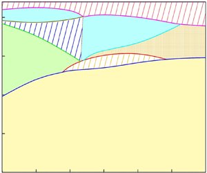
Figure 1 shows a schematic diagram of ETC in a two-dimensional concentric annulus due to charge injection and thermal buoyant force. The system consists of an outer cylinder with radius Ro, within which an inner cylinder with radius Ri is located in the centre, and the aspect ratio is fixed: A = 1.25. The inner and outer cylinders are kept at different constant temperatures θhot and θcold (Δθ 0 = θhot − θcold), respectively, and a radial direct current electric field is established by applying a voltage difference Δϕ 0 to the two electrodes. In this work, we assume that the fluid is incompressible, Newtonian, perfectly insulating and under the Boussinesq approximation. The free charges are only generated at the inner electrode and are then injected into the bulk of the liquid. A unipolar injection of the free charges is considered. It is also assumed that the injection is autonomous and homogenous (Laohalertdecha et al. Reference Laohalertdecha, Naphon and Wongwises2007), which means that the injected charge density q 0 at the inner cylinder remains constant and uniform.

Figure 1. Schematic diagram of ETC in a two-dimensional concentric annulus with A = 1.25. Red, yellow and blue are different regions divided.
The governing equations describing this problem include the Navier–Stokes equations, the temperature equation, the Poisson equation describing the electric potential and the charge conservation equation describing the charge transport. To further simplify the modelling, the viscous thermal dissipation, the magnetic effects and Joule heating are assumed to be negligible (Castellanos Reference Castellanos1998). We introduce dimensionless quantities, denoted with a star, as follows:
 \begin{equation}\left. {\begin{array}{*{20}{c@{}}} {x_i^\ast= \dfrac{x}{L},\quad u_i^\ast= \dfrac{u}{{\nu /L}},\quad {t^\ast } = \dfrac{t}{{{L^2}/\nu }},\quad {q^\ast } = \dfrac{q}{{{q_0}}},\quad {\phi^\ast } = \dfrac{\phi }{{\varDelta {\phi_0}}},}\\ {E_i^\ast= \dfrac{{{E_i}}}{{\varDelta {\phi_0}/L}},\quad {\theta^\ast } = \dfrac{{\theta - {\theta_{ref}}}}{{\varDelta {\theta_\textrm{0}}}},\quad {\rho^\ast } = \dfrac{\rho }{{{\rho_0}}},\quad {p^\ast } = \dfrac{p}{{{\rho_0}{{(\nu /L)}^2}}}} \end{array}}, \right\}\end{equation}
where L = Ro − Ri is the length scale. If we drop the superscript stars for clarity, the resulting governing equations of this ETC system are (Traoré et al. Reference Traoré, Pérez, Koulova and Romat2010)
 \begin{gather}\boldsymbol{\nabla }\boldsymbol{\cdot }\boldsymbol{u} = \textrm{0,}\end{gather}
 \begin{gather}\frac{{\partial \boldsymbol{u}}}{{\partial t}} + \boldsymbol{\nabla }\boldsymbol{\cdot }(\boldsymbol{uu}) =- \boldsymbol{\nabla }p + {\mathrm{\nabla }^\textrm{2}}\boldsymbol{u} + \frac{{Ra}}{{Pr}}\theta {\boldsymbol{e}_y} + {\left( {\frac{T}{M}} \right)^\textrm{2}}qC\boldsymbol{E},\end{gather}
 \begin{gather}\frac{{\partial \theta }}{{\partial t}} + \boldsymbol{\nabla }\boldsymbol{\cdot }(\theta \boldsymbol{u}) = \frac{1}{{Pr}}{\mathrm{\nabla }^\textrm{2}}\theta ,\end{gather}
 \begin{gather}{\mathrm{\nabla }^\textrm{2}}\phi =- Cq,\end{gather}
 \begin{gather}\boldsymbol{E} =- \boldsymbol{\nabla }\phi ,\end{gather}
 \begin{gather}\frac{{\partial q}}{{\partial t}} + \boldsymbol{\nabla }\boldsymbol{\cdot }\left[ {\left( {\frac{T}{{{M^2}}}\boldsymbol{E} + \boldsymbol{u}} \right)q} \right] = \frac{T}{{{M^2}}}\alpha {\mathrm{\nabla }^\textrm{2}}q.\end{gather}
In the above equations, u = (ux, uy) is the velocity, E = (Ex, Ey) is the electric field and ey is the vertical direction. The scalars ρ, θ, ϕ and q denote the fluid density, temperature, electric potential and charge density, respectively. Six dimensionless parameters appear in governing equations, defined as
 \begin{gather}
Ra = \frac{{g\beta \varDelta {\theta _0}{L^3}}}{{\nu \chi }}\textrm{,}\quad Pr
= \frac{\nu }{\chi },\quad T = \frac{{\varepsilon \varDelta
{\phi _\textrm{0}}}}{{\mu K}},\quad C =
\frac{{{q_0}{L^2}}}{{\varepsilon \varDelta {\phi
_\textrm{0}}}},\quad M = \frac{1}{K}{\left(
{\frac{\varepsilon }{{{\rho_0}}}} \right)^{1/2}},\notag\\
\alpha = \frac{D}{{K\varDelta {\phi
_\textrm{0}}}},
\end{gather}
\begin{gather}
Ra = \frac{{g\beta \varDelta {\theta _0}{L^3}}}{{\nu \chi }}\textrm{,}\quad Pr
= \frac{\nu }{\chi },\quad T = \frac{{\varepsilon \varDelta
{\phi _\textrm{0}}}}{{\mu K}},\quad C =
\frac{{{q_0}{L^2}}}{{\varepsilon \varDelta {\phi
_\textrm{0}}}},\quad M = \frac{1}{K}{\left(
{\frac{\varepsilon }{{{\rho_0}}}} \right)^{1/2}},\notag\\
\alpha = \frac{D}{{K\varDelta {\phi
_\textrm{0}}}},
\end{gather}
where the symbols μ, χ,  $\varepsilon$, K, β and D represent the dynamic viscosity, thermal diffusivity, electrical permittivity, ionic mobility, thermal expansion coefficient and charge diffusion coefficient, respectively. The Rayleigh number Ra and electric Rayleigh number T are the two driving parameters of the system. They represent the ratio of the buoyancy and Coulomb force to the viscous force, respectively. The Prandtl number Pr is defined as the ratio of the momentum diffusivity to the thermal diffusivity. The injection parameter C measures the strength of the charge injection. The dimensionless mobility parameter M is defined as the ratio of the so-called hydrodynamic mobility and the true mobility of the ions; α is the dimensionless ion diffusion number and the typical values of α are between 10−4 and 10−3 (Pérez & Castellanos Reference Pérez and Castellanos1989).
In addition, to characterize the heat transfer in the flow, Nusselt numbers are defined
 \begin{equation}N{u_i} = {R_i}\ \textrm{ln}\left( {\frac{{{R_o}}}{{{R_i}}}} \right){\left. {\frac{{\partial \theta }}{{\partial r}}} \right|_{r = {R_i}}},\quad N{u_o} = {R_o}\ \textrm{ln}\left( {\frac{{{R_o}}}{{{R_i}}}} \right){\left. {\frac{{\partial \theta }}{{\partial r}}} \right|_{r = {R_o}}},\end{equation}
in which Nui and Nuo denote local Nusselt numbers at the surfaces of the inner and outer cylinders. Then, the mean Nusselt number on each cylinder is computed by integration
 \begin{equation}\overline {N{u_i}} = \frac{\textrm{1}}{{\textrm{2}{\rm \pi} }}\int_\textrm{0}^{\textrm{2}{\rm \pi} } {N{u_i}(\delta )\,\textrm{d}\delta } ,\quad \overline {N{u_o}} = \frac{\textrm{1}}{{\textrm{2}{\rm \pi} }}\int_\textrm{0}^{\textrm{2}{\rm \pi} } {N{u_o}(\delta )\,\textrm{d}\delta } ,\end{equation}
where δ is the angle (see figure 1). Theoretically, the values of  $\overline {N{u_i}}$ and $\overline {N{u_o}}$ should be equal to each other due to energy conservation. However, a slight difference may be induced by the numerical error, so the final mean Nusselt number is defined as the average value of $\overline {N{u_i}}$ and $\overline {N{u_o}}$, i.e. $Nu = (\overline {N{u_i}} + \overline {N{u_o}} )/2$.
2.2. Linearization and global stability analysis
The linear problem is formulated following the work of He & Zhang (Reference He and Zhang2021) based on Reynolds’ decomposition  $\boldsymbol{N} = \bar{\boldsymbol{N}} + \boldsymbol{n^{\prime}}$, where N represents any flow variable discussed above, $\bar{\boldsymbol{N}}$ is the base state and $\boldsymbol{n^{\prime}}$ is the perturbation. After substituting the decompositions into the governing equations, subtracting from them the governing equations for the base states and retaining the terms of the first order, the linear system reads
 \begin{gather}\boldsymbol{\nabla }\boldsymbol{\cdot }\boldsymbol{u^{\prime}} = \textrm{0,}\end{gather}
 \begin{gather}\frac{{\partial \boldsymbol{u^{\prime}}}}{{\partial t}} + \boldsymbol{\nabla }\boldsymbol{\cdot }(\boldsymbol{u^{\prime}\bar{U}} + \boldsymbol{\bar{U}u^{\prime}}) =- \boldsymbol{\nabla }p^{\prime} + {\mathrm{\nabla }^2}\boldsymbol{u^{\prime}} + \frac{{Ra}}{{Pr}}\theta ^{\prime}{\boldsymbol{e}_y} + C{\left( {\frac{T}{M}} \right)^2}(q^{\prime}\bar{\boldsymbol{E}} + \bar{Q}\boldsymbol{e^{\prime}}),\end{gather}
 \begin{gather}\frac{{\partial \theta ^{\prime}}}{{\partial t}} + \boldsymbol{\nabla }\boldsymbol{\cdot }(\boldsymbol{u^{\prime}}\bar{\varTheta } + \bar{\boldsymbol{U}}\theta ^{\prime}) = \frac{1}{{Pr}}{\mathrm{\nabla }^2}\theta ^{\prime},\end{gather}
 \begin{gather}{\mathrm{\nabla }^2}\phi ^{\prime} =- Cq^{\prime},\end{gather}
 \begin{gather}\boldsymbol{e^{\prime}} =- \boldsymbol{\nabla }\phi ^{\prime},\end{gather}
 \begin{gather}\frac{{\partial q^{\prime}}}{{\partial t}} + \boldsymbol{\nabla }\boldsymbol{\cdot }\left[ {\left( {\frac{T}{{{M^2}}}\boldsymbol{e^{\prime}} + \boldsymbol{u^{\prime}}} \right)\bar{Q} + \left( {\frac{T}{{{M^2}}}\bar{\boldsymbol{E}} + \bar{\boldsymbol{U}}} \right)q^{\prime}} \right] = \frac{T}{{{M^2}}}\alpha {\mathrm{\nabla }^2}q^{\prime},\end{gather}
where  $\bar{\boldsymbol{U}}$, $\bar{\varTheta }$, $\bar{\varPhi }$ and $\bar{Q}$ are the base states of velocity, temperature, electrical potential and charge density, respectively, and $\boldsymbol{u^{\prime}}$, $\theta ^{\prime}$, $\phi ^{\prime}$, $q^{\prime}$ are the corresponding perturbation fields. The boundary condition for the fluctuations on the two impermeable isothermal walls given by
 \begin{equation}\left. {\begin{array}{*{20}{c@{}}} {\boldsymbol{u^{\prime}}{|_{r = {R_i}}} = 0,\quad \theta^{\prime}{|_{r = {R_i}}} = 0,\quad \phi^{\prime}{|_{r = {R_i}}} = 0,\quad q^{\prime}{|_{r = {R_i}}} = 0,}\\ {\boldsymbol{u^{\prime}}{|_{r = {R_o}}} = 0,\quad \theta^{\prime}{|_{r = {R_o}}} = 0,\quad \phi^{\prime}{|_{r = {R_o}}} = 0,\quad {{\left. {\dfrac{{\partial q^{\prime}}}{{\partial r}}} \right|}_{r = {R_o}}} = 0.} \end{array}} \right\}\end{equation}
In the linear stability analysis, it is a common practice to rewrite the fluid system in the form of a matrix; see the work of He & Zhang (Reference He and Zhang2021). Therefore, (2.11)–(2.16) can be written in a compact manner as
 \begin{equation}\frac{{\partial \boldsymbol{n^{\prime}}}}{{\partial t}} = \boldsymbol{Mn^{\prime}},\end{equation}
where M represents the linearized Navier–Stokes operator for the ETC in the annulus and  $\boldsymbol{n^{\prime}} = {({v^\prime },\eta ^{\prime},\phi ^{\prime},\theta ^{\prime})^T}$, $v^{\prime}$ and $\eta ^{\prime}$ are the wall-normal velocity and wall-normal vorticity, respectively. In the temporal stability analysis, a wave-like solution (Schmid, Henningson & Jankowski Reference Schmid, Henningson and Jankowski2002) $\boldsymbol{n^{\prime}} = \hat{n}(x,y)\,{\textrm{e}^{ - \textrm{i}\omega t}}$ is assumed, leading to an eigenvalue problem that reads as
 \begin{equation}- \textrm{i}\omega \hat{n} = \boldsymbol{M}\hat{n}, \end{equation}
where −iω is the eigenvalue and  $\hat{n}$ is the corresponding eigenvector. The complex-valued ω is the circular frequency of the perturbation, with its real part ωr representing the phase speed and its imaginary part ωi representing the growth rate of the linear perturbation. If ωi = 0 when ωr vanishes, it is said that an exchange of stabilities occurs, and the flow makes a transition to another steady state. Such a transition can be classified into pitchfork bifurcations, saddle-node bifurcations and transcritical bifurcations according to bifurcation theory (Crawford Reference Crawford1991). If ωr ≠ 0 when ωi vanishes, the steady solution is unstable to an oscillatory disturbance (this behaviour was named ‘overstability’ by Eddington Reference Eddington1920), and it makes a transition to a periodic solution with the angular velocity ωr. Such a transition is called a Hopf bifurcation.
To solve the eigenvalue problem, the matrix-free method (Theofilis Reference Theofilis2011) is engaged by using time-stepping methods, which employ temporal integrations of the perturbations using the linear Navier–Stokes equations,  ${\partial _t}\boldsymbol{n^{\prime}} = \boldsymbol{Mn^{\prime}}$, from 0 to t. This is equivalent to applying the exponential operator $\textrm{exp}(\int_0^t \boldsymbol{M} \,\textrm{d}t)$ to the perturbation $\boldsymbol{n^{\prime}}$. Thus, the eigenvalue problem to be solved using the time-stepping method is defined by the exponential operator of the linearized version of the equations. The leading eigenvalue of the exponential operator to which the power method converges is usually the most unstable eigenvalue of the linearized operator.
2.3 Linearized lattice Boltzmann methods
To discover the full bifurcation diagram of the annular ETC, we need to simultaneously solve the fully coupled nonlinear equations (2.2)–(2.7) and linearized equations (2.11)–(2.16). Instead of directly solving the governing equations at the macroscopic level, here, we perform both the direct numerical simulation (DNS) and global linear stability analysis in the framework of the mesoscopic lattice Boltzmann method (LBM). As the LBM for the DNS of this problem has been well studied (Luo et al. Reference Luo, Wu, Yi and Tan2016a,Reference Luo, Wu, Yi and Tanb; Lu, Liu & Wang Reference Lu, Liu and Wang2019), we focus on the derivation of a LLBM solver for the linearized governing equations. In our LLBM model, a standard Bhatnagar–Gross–Krook scheme (Guo, Shi & Wang Reference Guo, Shi and Wang2000) was employed for all fields, including the perturbation flow, perturbation electric potential, perturbation charge density and perturbation temperature.
For the perturbation flow and perturbation temperature, the LLBM equations have been built for the global linear stability analysis of incompressible flows (Pérez et al. Reference Pérez, Aguilar and Theofilis2017) and thermal convective flows (Jiang et al. Reference Jiang, Luo, Zhang, Wu and Yi2022), under D2Q9 (two-dimensional nine-velocity) velocity discretization, and are formulated as follows:
 \begin{gather}{f_i}(\boldsymbol{x} + {\boldsymbol{e}_i}\varDelta t,t + \varDelta t) - {f_i}(\boldsymbol{x},t) =- \frac{1}{{{\tau _v}}}[\,{f_i}(\boldsymbol{x},t) - f_i^{eq}(\boldsymbol{x},t)] + \varDelta t{F_i}(\boldsymbol{x},t),\end{gather}
 \begin{gather}{l_i}(\boldsymbol{x} + {\boldsymbol{e}_i}\varDelta t,t + \varDelta t) - {l_i}(\boldsymbol{x},t) =- \frac{1}{{{\tau _\theta }}}[{l_i}(\boldsymbol{x},t) - l_i^{eq}(\boldsymbol{x},t)],\end{gather}
where f and l are the distribution functions of the perturbation fluid density and perturbation temperature, respectively. The relaxation times  ${\tau _v}$ and ${\tau _\theta }$ are defined as
 \begin{equation}{\tau _v} = \frac{{3\nu }}{{{c^2}\varDelta t}} + \frac{1}{2},\quad {\tau _\theta } = \frac{{3\chi }}{{{c^2}\mathrm{\Delta }t}} + \frac{1}{2}.\end{equation}
 The corresponding equilibrium distributions  $f_i^{eq}$ and $l_i^{eq}$, and the source terms Fi in (2.20) and (2.21) are formulated (Pérez et al. Reference Pérez, Aguilar and Theofilis2017; Jiang et al. Reference Jiang, Luo, Zhang, Wu and Yi2022) as
 \begin{gather}f_i^{eq} = \frac{{\rho ^{\prime}}}{{\bar{\rho }}}\bar{f}_i^{eq}\textrm{ + }\bar{\rho }{w_i}\left[ {\frac{{{\boldsymbol{e}_i} \boldsymbol{\cdot} \boldsymbol{u^{\prime}}}}{{c_s^2}} + \frac{{({\boldsymbol{e}_i} \boldsymbol{\cdot} \boldsymbol{u^{\prime}})({\boldsymbol{e}_i}\boldsymbol{\cdot }\bar{\boldsymbol{U}})}}{{c_s^4}} - \frac{{\boldsymbol{u^{\prime}} \boldsymbol{\cdot} \bar{\boldsymbol{U}}}}{{c_s^2}}} \right],\end{gather}
 \begin{gather}\bar{f}_i^{eq} = \bar{\rho }{w_i}\left[ {1 + \frac{{{\boldsymbol{e}_i}\boldsymbol{\cdot }\bar{\boldsymbol{U}}}}{{c_s^2}} + \frac{{{{({\boldsymbol{e}_i}\boldsymbol{\cdot }\bar{\boldsymbol{U}})}^2}}}{{c_s^4}} - \frac{{{{\bar{\boldsymbol{U}}}^2}}}{{c_s^2}}} \right],\end{gather}
 \begin{gather}l_i^{eq} = \frac{{\theta ^{\prime}}}{{\bar{\varTheta }}}\bar{l}_i^{eq} + \bar{\varTheta }{w_i}\left[ {\frac{{{\boldsymbol{e}_i}\boldsymbol{\cdot }\boldsymbol{u^{\prime}}}}{{c_s^2}} + \frac{{({\boldsymbol{e}_i}\boldsymbol{\cdot }\boldsymbol{u^{\prime}})({\boldsymbol{e}_i}\boldsymbol{\cdot }\bar{\boldsymbol{U}})}}{{c_s^4}} - \frac{{\boldsymbol{u^{\prime}}\boldsymbol{\cdot }\bar{\boldsymbol{U}}}}{{c_s^2}}} \right],\end{gather}
 \begin{gather}\bar{l}_i^{eq} = \bar{\varTheta }{w_i}\left[ {1 + \frac{{{\boldsymbol{e}_i}\boldsymbol{\cdot }\bar{\boldsymbol{U}}}}{{c_s^2}} + \frac{{{{({\boldsymbol{e}_i}\boldsymbol{\cdot }\bar{\boldsymbol{U}})}^2}}}{{c_s^4}} - \frac{{{{\bar{\boldsymbol{U}}}^2}}}{{c_s^2}}} \right],\end{gather}
 \begin{gather}{F_i} = {w_i}\left( {1 - \frac{1}{{2{\tau_v}}}} \right)\frac{{{\boldsymbol{e}_i}\{ \boldsymbol{g}\beta [\bar{\rho }\theta ^{\prime} + \rho ^{\prime}(\bar{\varTheta } - {{\bar{\varTheta }}_{ref}})] + q^{\prime}\bar{\boldsymbol{E}} + \bar{Q}\boldsymbol{e^{\prime}}\} }}{{c_s^2}},\end{gather}
and the macroscopic quantities are calculated through (2.26), as follows:
 \begin{gather}\rho ^{\prime} =
\sum\limits_i {{f_i}} ,\;\;\bar{\rho
}\boldsymbol{u^{\prime}} + \rho ^{\prime}\bar{U} =
\sum\limits_i {{\boldsymbol{e}_i}{\,f_i} + \frac{{\Delta
t}}{2}\{ \boldsymbol{g}\beta [\bar{\rho }\theta ^{\prime} +
\rho ^{\prime}(\bar{\varTheta } - {{\bar{\varTheta
}}_{ref}})] + q^{\prime}\bar{\boldsymbol{E}} +
\bar{Q}\boldsymbol{e^{\prime}}\} } ,\notag\\ \theta ^{\prime} =
\sum\limits_i
{{l_i}.}\end{gather}
\begin{gather}\rho ^{\prime} =
\sum\limits_i {{f_i}} ,\;\;\bar{\rho
}\boldsymbol{u^{\prime}} + \rho ^{\prime}\bar{U} =
\sum\limits_i {{\boldsymbol{e}_i}{\,f_i} + \frac{{\Delta
t}}{2}\{ \boldsymbol{g}\beta [\bar{\rho }\theta ^{\prime} +
\rho ^{\prime}(\bar{\varTheta } - {{\bar{\varTheta
}}_{ref}})] + q^{\prime}\bar{\boldsymbol{E}} +
\bar{Q}\boldsymbol{e^{\prime}}\} } ,\notag\\ \theta ^{\prime} =
\sum\limits_i
{{l_i}.}\end{gather} The electrical part equations, including the Poisson equation for perturbation electric potential  $\phi ^{\prime}$ and Nernst–Plank equation for the perturbation charge density $q^{\prime}$, are also modelled by LLBMs. Here, the improved lattice Boltzmann model for the Poisson equation proposed by Chai & Shi (Reference Chai and Shi2008) is used to solve $\phi ^{\prime}$, and the corresponding lattice Boltzmann equation (LBE) can be given as
 \begin{equation}{g_i}(\boldsymbol{x} + {\boldsymbol{e}_i}\varDelta t,t + \varDelta t) - {g_i}(\boldsymbol{x},t) =- \frac{1}{{{\tau _\phi }}}[{g_i}(\boldsymbol{x},t) - g_i^{eq}(\boldsymbol{x},t)] + \varDelta t{\varpi _i}R{D_a},\end{equation}
where g, e,  ${\tau _\phi }$, R and Da are distribution functions, microscopic velocity, relaxation time, source term and artificial diffusion coefficient, respectively. The D2Q5 (two-dimensional five-velocity) velocity discretization is adopted for the electric potential, with the equilibrium distribution function $g_i^{eq}$ and the corresponding weight coefficients ω and ϖ being expressed as
 \begin{gather}g_i^{eq}(\boldsymbol{x},t) = \left\{ {\begin{array}{@{}ll@{}} {({\omega_0} -
1.0)\phi^{\prime}}&{i = 0}\\ {{\omega_i}\phi^{\prime}}&{i =
1 - 4} \end{array}} \right.,\quad {\omega _i} = \left\{
\begin{array}{@{}ll@{}} 0&{i = 0}\\ {1/4}&{i = 1 - 4}
\end{array}\right.,\notag\\ {\varpi_i} = \left\{
{\begin{array}{@{}ll@{}} 0&{i = 0}\\ {1/4}&{i = 1 - 4}
\end{array}}. \right.\end{gather}
\begin{gather}g_i^{eq}(\boldsymbol{x},t) = \left\{ {\begin{array}{@{}ll@{}} {({\omega_0} -
1.0)\phi^{\prime}}&{i = 0}\\ {{\omega_i}\phi^{\prime}}&{i =
1 - 4} \end{array}} \right.,\quad {\omega _i} = \left\{
\begin{array}{@{}ll@{}} 0&{i = 0}\\ {1/4}&{i = 1 - 4}
\end{array}\right.,\notag\\ {\varpi_i} = \left\{
{\begin{array}{@{}ll@{}} 0&{i = 0}\\ {1/4}&{i = 1 - 4}
\end{array}}. \right.\end{gather} The relaxation time  ${\tau _\phi }$ and source term R can be computed from
 \begin{equation}{\tau _\phi } = \frac{{{D_a}}}{{\beta {c^2}\varDelta t}} + \frac{1}{2},\quad R = Cq.\end{equation}
The artificial diffusion coefficient Da (Da > 0) is chosen to be Da = 1/2 to balance the evolution speed and numerical stability. The coefficient β has been derived to be 1/2 by the Chapman–Enskog expansion (Chai & Shi Reference Chai and Shi2008). Finally, the electric potential and charge density can be evaluated as
 \begin{equation}\phi ^{\prime} = \frac{1}{{1 - {\omega _0}}}\sum\limits_{i = 1}^4 {{g_i}} .\end{equation}
 The LLBM for perturbation charge density  $q^{\prime}$ is more complex because (2.16) is inherently nonlinear as the electric field E is a function of q. It is noticed that (2.16) has the form of a convection–diffusion equation (CDE). In the adoption of LBM for solving the CDE (Shi & Guo Reference Shi and Guo2009; Chai & Shi Reference Chai and Shi2020; Zhao et al. Reference Zhao, Wu, Chai and Shi2020; Chen et al. Reference Chen, Chai, Shang and Shi2021; Wang et al. Reference Wang, Wei, Li, Chai and Shi2021a; Chai, Shi & Zhan Reference Chai, Shi and Zhan2022), the nonlinear charge mobility term can be treated as a cross-diffusion term (Wang et al. Reference Wang, Wei, Li, Chai and Shi2021a) or a convective term (Chai et al. Reference Chai, Shi and Zhan2022); these two models show almost no difference in this problem. Here, we can build the LLBM for $q^{\prime}$ by treating the nonlinear charge mobility term inspired by the work of Wang et al. (Reference Wang, Wei, Li, Chai and Shi2021a). Under D2Q9 (two-dimensional nine-velocity) velocity discretization, we have
 \begin{equation}{h_i}(\boldsymbol{x} + {\boldsymbol{e}_i}\varDelta t,t + \varDelta t) - {h_i}(\boldsymbol{x},t) =- \frac{1}{{{\tau _q}}}[{h_i}(\boldsymbol{x},t) - h_i^{eq}(\boldsymbol{x},t)] + \varDelta t{G_i} + \varDelta t{S_i},\end{equation}
where  $h_i^{eq}$ is the equilibrium distribution function, Gi is the term to recover the cross-diffusion term and Si is the correction term to eliminate the additional terms appearing in the recovered macroscopic equations (Wang et al. Reference Wang, Wei, Li, Chai and Shi2021a,Reference Wang, Yang, Wang, Chai and Weib). We further have
 \begin{gather}h_i^{eq} = \frac{{q^{\prime}}}{{\bar{Q}}}\bar{h}_i^{eq} + \bar{Q}{w_i}\frac{{{\boldsymbol{e}_i} \boldsymbol{\cdot} \boldsymbol{u^{\prime}}}}{{c_s^2}},\quad \bar{h}_i^{eq} = \bar{Q}{w_i}\left[ {1 + \frac{{{\boldsymbol{e}_i} \boldsymbol{\cdot} \bar{\boldsymbol{U}}}}{{c_s^2}}} \right],\quad {\tau _q} = \frac{{\alpha T\nu }}{{{M^2}c_s^2\mathrm{\Delta }t}} + \frac{1}{2},\end{gather}
 \begin{gather}\boldsymbol{G} =- \left( {\frac{T}{{{M^2}}}} \right)\frac{{\bar{Q}\boldsymbol{\nabla }\phi ^{\prime} + q^{\prime}\boldsymbol{\nabla }\bar{\varPhi }}}{{{\tau _q}\varDelta t}},\quad {G_i} = \frac{{{w_i}{\boldsymbol{e}_i}}}{{c_s^2}} \boldsymbol{\cdot} \boldsymbol{G}\end{gather}
 \begin{gather}\boldsymbol{S} = \left( {1 - \frac{1}{{2{\tau_q}}}} \right){\partial _t}(\boldsymbol{u^{\prime}}\bar{Q}\boldsymbol{+ \bar{U}}q^{\prime}),\quad {S_i} = \frac{{{w_i}{\boldsymbol{e}_i}}}{{c_s^2}}\boldsymbol{\cdot }\boldsymbol{S}, \end{gather}
and the charge density is evaluated from
 \begin{equation}q^{\prime} = \sum\limits_j {{h_j}} .\end{equation}
Theoretically, we need to recover the linearized governing equations by Chapman–Enskog (CE) expansion. Pérez et al. (Reference Pérez, Aguilar and Theofilis2017) first recovered the linearized Navier–Stokes equation without an external force from the LBE by a CE analysis. Recently, we have extended Pérez's model for the global instability analysis of thermal convection (Jiang et al. Reference Jiang, Luo, Zhang, Wu and Yi2022) with the CE expansion. Besides, the CE analysis of Poisson-type perturbation charge potential equation can be found in the work of Chai & Shi (Reference Chai and Shi2008). Finally, the CE analysis of perturbation charge density equation is provided in Appendix A.
2.4 Fractal dimension and Lyapunov exponent
In this paper, the fractal dimension and Lyapunov exponent are adopted to further test the chaos quantitatively. The fractal dimension dc measures the degrees of freedom associated with hydrodynamics, given by
 \begin{equation}{d_c} = \mathop {\lim }\limits_{s \to 0} \frac{{\log ({C_p}(s))}}{{\log (s)}},\end{equation}
where correlation function Cp(s) represents the minimum number of hyper cubes (of size s) covering a given set of points in a p-dimensional space, divided by N 2 (N being the number of samples), and is defined as
 \begin{equation}{C_p}(s) = \mathop {\lim }\limits_{N \to \infty } \frac{1}{{{N^2}}}\sum\limits_{\scriptstyle i,j = 1 \atop \scriptstyle i \ne j}^N {h(s - |{\boldsymbol{X}_i} - {\boldsymbol{X}_j}|)} ,\end{equation}
in which h is the Heaviside function,  ${\boldsymbol{X}_i}$ and ${\boldsymbol{X}_j}$ are a pair of given data points. The straight part of the curves for Cp(s) as a function of s on log–log scale will tend to have a constant slope as p increases. In particular, the slope of the periodic flow is close to 1, the slope of the quasi-periodic flow is close to 2 and the slope of the chaos is a real number greater than 2 (Grassberger & Procaccia Reference Grassberger and Procaccia1983).
The algorithm of Wolf et al. (Reference Wolf, Swift, Swinney and Vastano1985) is used for estimating the maximum Lyapunov exponent from time traces of the temperature at sampling point P. Since the implementation of this algorithm is relatively complicated, only a simple description is given here. For more details of this algorithm, interested readers can refer to Wolf et al. (Reference Wolf, Swift, Swinney and Vastano1985). Generally, for a given time series {x 1, x 2, …, xk, …}, its reconstructed phase space (dimension N) can be described as
 \begin{equation}Y({t_i}) = [x({t_i}),x({t_i} + {\tau _L}), \ldots ,x({t_i} + ({n_{dim}} - 1){\tau _L})],\quad i = 1,2, \ldots ,N,\end{equation}
in which ndim is the number of embedding dimensions, τL represents the delay time. We follow the evolution in time of the initial point Y(t 0) of the trajectory and its nearest point Y 0(t 0) belonging to a different portion of the trajectory. Then, the distance between these two points changes continuously over time. At time t 1, the distance between these two points changes from L(t 0) = |Y(t 0) − Y 0(t 0)| to L(t 1) = |Y(t 1) − Y 0(t 1)|, then another point Y 1(t 1) of the trajectory is selected to keep the distance |Y 1(t 1) − Y 0(t 1)| = L(t 0). Repeat the above process until YE(tE) reaches the end of the time series; at this time, the total number of iterations is E. If the value of E is large enough, then the maximum Lyapunov exponent can be obtained by
 \begin{equation}{\lambda _{max}} = \frac{1}{{{t_E} - {t_0}}}\sum\limits_{k = 0}^E {\frac{{L({t_k})}}{{L({t_0})}}} .\end{equation}
It should be noted that the corresponding dynamical system is chaotic when the maximum Lyapunov exponent λmax is positive (Rempel & Chian Reference Rempel and Chian2007). The larger the positive exponent, the more chaotic the system is.
2.6. Numerical method
Both the DNS and the solving of linear Navier–Stokes equations of the ETC are performed using the computational fluid dynamics solver Palabos (Latt et al. Reference Latt2021), which is well known for its efficient parallelization and second-order accuracy. In the current work, the time step Δt is determined by the Courant–Friedrichs–Lewy condition with the target Courant number being 0.005. The mesoscopic boundary conditions of non-equilibrium extrapolation (Guo, Zheng & Shi Reference Guo, Zheng and Shi2002a,Reference Guo, Zheng and Shib) are used.
3. Validation
The grid independence test and basic validation results of DNS are shown in Appendix B. Here, the accuracy of the solution of the linear equations (2.17)–(2.22) using the LLBM solver was tested by calculating the linear stability criteria. Figure 2(a1,a2) shows the spatial distribution of the base flow and the leading global mode for natural convection (without the electric effect) at Pr = 0.0733, Ra = 1608.8 and A = 1.25. It was detected that the change of sign of the exponent ωi occurs approximately at the critical value Rac = 2472. Our numerical results are in fairly good agreement with the data of Serrano-Aguilera et al. (Reference Serrano-Aguilera, Blanco-Rodríguez and Parras2021) (Rac = 2438 by a spectral method), with a relative error of 1.39%.

Figure 2. Base flows (first row) and their corresponding most unstable mode (second row). (a) Natural convection at Pr = 0.0733, Ra = 1608.8 and A = 1.25; (b) electrohydrostatic state at T = 120, k = 8 and A = 2; (c) electroconvection state at T = 120 and A = 2.
Then, we verified the linear critical Tc of pure electric convection for both the first bifurcation and the second bifurcation. Figure 3 shows the neutral curve of the first bifurcation for modes k = 6, 7, 8 and 9 as a function of A at C = 10, M = 10 and α = 10−3. At the same parameter condition, Wu et al. (Reference Wu, Vázquez, Traoré and Pérez2014) obtained the linear criterion as Tc 1 = 122 for mode k = 8 with A = 2 and α = 0. We find that the current Tc 1 = 119.8 at A = 2 is lower than the linear stability criterion. Figure 2(b1) shows the electrohydrostatic state at T = 120 and figure 2(b2) gives the leading mode for k = 8, which is similar to the results of Pérez et al. (Reference Pérez, Vázquez, Wu and Traoré2014). After the emergence of EC, due to the competition between the ionic velocity and fluid velocity (Castellanos, Atten & Perez Reference Castellanos, Atten and Perez1987), the flow is characterized by eight pairs of charge-void regions (where the value of q is almost zero in figure 2c1). As T continues to increase, the second bifurcation occurs. There has been no linear instability analysis of the second instability, and only DNSs were used to calculate the criterion by Huang et al. (Reference Huang, Wang, Guan, Du, Deepak Selvakumar and Wu2021), who obtained Tc 2 = 213 for eight cells under parameters A = 2, M = 5, C = 10 and α = 0. We obtain the linear results as Tc 2 = 242 with α = 10−3 (the eigenfunction q of the most unstable mode is shown in figure 2c2).

Figure 3. Linear critical values Tc 1 of modes k = 6, 7, 8 and 9 as a function of A/(A + 2) at α = 10−3.
We find that the current Tc 1 and Tc 2 are lower and higher than the linear stability criterion obtained from the finite volume method, which neglected the charge diffusion effect. Here, we attribute this discrepancy to the effects of charge diffusion. Zhang et al. (Reference Zhang, Martinelli, Wu, Schmid and Quadrio2015, 2016) analysed the linear and weakly nonlinear stability of EC of dielectric liquids subjected to strong unipolar injection with the charge diffusion effect considered. It was found that the charge diffusion can destabilize the linearized EC but stabilizes the flow in an early phase of the nonlinear development of the disturbance, which means that weaker charge diffusion leads to greater Tc 1 and smaller Tc 2, consistent with the comparison here. The quantitative effects of α on Tc for the first and second bifurcations are shown in figure 4. This dual effect of charge diffusion has also been discussed by Castellanos, Pérez & Atten (Reference Castellanos, Pérez and Atten1989) in their DNS of such flows.

Figure 4. Effect of α on the criteria Tc of (a) the first bifurcation at A = 2 and M = 10; (b) the second bifurcation at A = 2 and M = 5.
4. Results and discussion
4.1. DNS
These parameters are fixed for all following cases: A = 1.25, C = 10, Pr = 10, M = 5 and α = 10−3. To study the effect of the radial electric field on the pure thermal convection in the concentric annulus, the first problem to be addressed is the determination of steady-state solutions in a Ra–T map, as shown in figure 5. To obtain this map, we visited the different positions of Ra ∈ [0, 3 × 10⁴] and T ∈ [0, 220] by dividing the map into 30 and 22 points, respectively. Therefore, this study aimed to provide a steady solution for 660 cases in the range of Ra and T investigated. Here, Ra is fixed and we increase T from zero; we solve for the steady-state solution by means of the Newton–Raphson iteration using as the initial guess the final-time result obtained from the previous simulations at lower T. As shown in figure 5, the solution region is divided into three flow states (seven subregions). The number of thermal plumes ‘P×’, the number of charge-void regions ‘C×’ and the stable/unstable flow state ‘S/U’ constitute the name of every subregion, i.e. the P1-C0-S solution represents steady convection with a main thermal plume at the top of the annulus without a charge-void region. Chaos is represented by the yellow dot region.

Figure 5. Map of flow patterns for ETC in a two-dimensional concentric annulus.
From the dimensionless momentum equation (2.2), the total destabilizing effect from electric and thermal forces along the radial direction is
 \begin{equation}{F_r} = |{C{T^2}\,Pr\,q\boldsymbol{E}+{M^2}Ra\theta \,\textrm{cos}(\delta )} |.\end{equation}
Compared with the plate–plate configuration, the electrothermo-convective phenomenon in the cylindrical configuration is much more complex. This is partially due to the differences in the directions of the driving forces and the basic flow patterns. From (4.1), the Rayleigh–Bénard thermal instability can be enhanced by destabilizing the electric field occurring in the top part of the thermally unstable region (red shadow region with δ < 45°); hydrodynamic instability can occur in the vertical section (yellow shadow regions with δ near 90°), which is called ‘natural convection heated from sidewalls’; and the instability caused by the baroclinic torque at the bottom of the annulus (red shadow region), as shown in figure 1. Therefore, instability of ETC in the annulus may be a combination of these mechanisms.
4.1.1. Bifurcations and multiple solutions with Ra
We keep T constant but different from zero (select three cases: T = 50, 100 and 150) and vary the Rayleigh number in such a way as to cross the critical line in a direction parallel to the Ra axis. Yoo (Reference Yoo1999) first researched the saddle-node bifurcation for natural convection in an annulus when Pr > 0.5. The P1-C0-S solution tends to be excited more easily at zero-field initial conditions, and the P2-C1-S solution branch can be obtained with the help of artificial numerical disturbances, which were introduced during a short initial period (t < 0.01) to enhance the separation of the boundary layer from a point other than the top of the inner cylinder for one plume case. Saddle-node bifurcation occurs at Ra > Ras = 2024 for the case of T = 50, where the P1-C0-S solution branch and P2-C1-S solution branch are independent of each other, as shown in the bifurcation diagram in figure 6(a). As Ra continues to rise, the P2-C1-S solution transitions to an oscillatory state at Rac = 15 423; however, the P1-C0-S solution remains stable.

Figure 6. The mean Nu changes over Ra for three different T; (a) T = 50 (dotted lines represent the oscillation), (b) T = 100 with red coloured lines (increasing Ra), blue coloured lines (decreasing Ra) and T = 150 with green coloured lines (green points represent the chaos state).
Figure 6(b) shows the relation between Nu and Ra at T = 100 and T = 150. The saddle-node bifurcation disappears and is replaced by subcritical bifurcation at these two electric Rayleigh numbers. At T = 150, the P5-C5-S solution remains steady until Ra > Rac = 12 435, just like the case shown in figure 7(a). Then, infinite local maximum and minimum amplitudes of Nu indicate that steady convection transitions to the disorder state. Complex transition processes and hysteresis phenomena occur in the case of T = 100, and we summarize them as follows:
(i) The P5-C5-S solution possesses a symmetrical distribution along the vertical centreline at Ra < Rac 1 = 5468, as shown in figure 7(a). The value of Fr decreases as Ra increases when δ > 90° from (4.1). At Ra = Rac 1, the strength of the electric plume does not maintain the existence of a charge-void region in the bottom of the annulus, and the P5-C5-S solution bifurcates to the P5-C4-S solution, as shown in figure 7(b).
(ii) The intensity of the main plume Pm (one plume with maximum flow intensity) continually increases with Ra and squeezes the room taken by secondary thermal plumes Ps (other plumes except Pm), so charge-void regions Cs (corresponding to Ps) move along the −y-direction for the P5-C4-S solution. Identically, these two charge-void regions will disappear once the magnitude of Fr is less than the critical finite amplitude at Ra > Rac 2 = 7066. Figure 7(c) shows the distribution of the P3-C2-S solution after this transition.
(iii) Different from the former two processes, no plume suffers from the inhibition of the stabilizing buoyancy force for the P3-C2-S solution. Two large charge-void regions Cm (corresponding to Ps) are stable and fixed at their location with increasing Ra (<Rac 3). Figure 6(a) indicates that multiple plume structures are more unstable than a single plume. When Ra > Rac 3 = 17 323, the P3-C2-S solution is broken and then convection transitions to the P1-C0-S state (in figure 7d) through a phase of chaos.
(iv) The hydrodynamic behaviours of this ETHD system with continually decreasing Ra can be understood as a reverse process of increasing Ra. The magnitude of Fr rises with the decline in Ra, and new charge-void regions occur at a special Raf at the bottom of the annulus. Therefore, the P5-C4-S and P3-C2-S solutions bifurcate to the P5-C5-S state at Raf 1 = 2506 and Raf 2 = 712, respectively. The P1-C0-S state first transitions to the P3-C2-S solution at Raf 3 = 2820 and then returns to the P5-C5-S solution at Raf 2.

Figure 7. Four solutions at Ra = 5000 and T = 100. Panels (a–d) are the finite-amplitude solutions corresponding to the P5-C5-S, P5-C4-S, P3-C2-S and P1-C0-S solution branches, respectively.
4.1.2. Bifurcations and heat transfer enhancement with T
The next research question is investigation of the hydrodynamics of this ETC by varying T instead of Ra. We consider the case of Ra = 5000; to more clearly depict the subcritical feature, the bifurcation diagram is drawn in figure 8. Three hysteresis loops can be observed. The explanations are as follows:
(i) The P1-C0-S solution can be obtained from the zero-field initial condition at T = 0. Increasing T until T > Tc 1 = 122, the instability exchange and the flow transition to the P5-C5-S solution branch (in figure 7a). An interesting transition occurs at T = 187, where the P5-C5-S solution loses its stability and all charge-void regions travel clockwise. We discuss this instability mechanism in the next section. However, the P5-C5-S state bifurcation to a P6-C6-S state is shown in the enlarged inset of figure 8 at T = 192. Then, the P6-C6-S solution transitions to the travelling wave state when T > Tc 5 = 201.
(ii) Saddle-node bifurcation is proven in the ETHD system with a low electric Rayleigh number, as shown in figure 6(a), and we also obtain a P2-C1-S solution branch at T = 0. This P2-C1-S state is more stable than P1-C0-S, which bifurcates to the P5-C5-S solution at T > Tc 2 = 129.
(iii) The P6-C6-S solution transitions to the P3-C2-S state (in figure 7c) with the disappearance of four charge-void regions at T < Tf 1 = 99. These two charge-void regions cannot be maintained when T < Tf 2 = 62 and the flow returns to the P1-C0-S state. Moreover, the P3-C2-S solution can be a saddle-node bifurcation solution branch, which bifurcates to the P5-C5-S solution at Tc 3 = 111.

Figure 8. The mean Nu over T at Ra = 5000. The shaded area shows the enhanced heat transfer caused by the P6-C6-S solution compared with the P1-C0-S solution. The blue lines represent decreasing T continually.
In summary, this ETHD system consists of saddle-node bifurcations, subcritical bifurcations and supercritical bifurcations. Two conclusions can be drawn about the heat transfer from these determined bifurcation routes. First, the Nusselt number decreases with increasing Ra when thermal plumes exist in the lower part of the annulus. Second, the heat transfer efficiency is connected to the number of plumes under the same drive parameters, as shown in figures 6 and 8. Six plumes had the largest Nusselt number Nu = 2.90; however, the Nusselt number was only equal to 1.70 when only one plume existed, as shown in figure 7. Moreover, we can enhance the heat transfer in a determined manner: with the zero-field initial condition, we first increase the electric Nusselt number until T > Tc 1 and then decrease T to the value that we need.
4.2. Global linear instability analysis
The transition of multiple plume solutions (more than two plumes) is explained by analysing the magnitude of Fr at the bottom of the annulus successfully. However, it cannot explain the transition behaviour of the single and two-plume solutions (P1-C0-S and P2-C1-S) on the saddle-node bifurcation branches shown in figures 6(a) and 8. In this section, we carry out a global linear instability analysis by analysing the spectrum of the eigenvalues of the operator M. Due to the symmetry of the boundary condition, the two-dimensional base flow admits the symmetry property about the x = 0 line, i.e. Φb(x, y, t) = Φb(−x, y, t) with Φ = [u, v, θ, q, ϕ]. Solutions φ of the linearized Navier–Stokes equations admit the following two types of symmetry with respect to the x = 0 plane:
 \begin{gather}\textrm{S-mode}\quad\varphi (x,y,t) = \varphi ( - x,y,t),\end{gather}
 \begin{gather}\textrm{A-mode}\quad \varphi (x,y,t) =- \varphi ( - x,y,t).\end{gather}
Figure 9(a,b) illustrates the behaviour of eigenvalues in figure 6(a) with T = 50 and Ra ∈ [14 500, 15 300]. Eigenpairs are extracted by adding a random symmetry/anti-symmetry perturbation about the x = 0 line as the initial condition. We only give the S-mode (leading mode) solution here because the A-mode has a too rapid damping rate with time to be extracted. The P1-C0-S solution reflects a rapid decline with monotonic instability in this parameter range. However, this instability of the P1-C0-S solution will be replaced with overstability because the flow is thermally dominant, where the magnitude of buoyancy is approximately 4.5 times larger than the electric force from (4.1). Therefore, instability of the P1-C0-S solution is similar to the case of pure thermal convection discussed by Serrano-Aguilera et al. (Reference Serrano-Aguilera, Blanco-Rodríguez and Parras2021), who proved that the S-mode is the most unstable mode and the bifurcation is Hopf type, which is consistent with our conclusion. For the P2-C1-S solution, it shows an overstability with a critical angular frequency ωr = 12.07 at Rac = 15 423 and the corresponding distribution of eigenfunctions θ and q are shown in figures 10(a1) and 10(a2). The eigenfunction θ has its maxima at an approximate angle of 45° in the lower region of the ascending jets, so these parts will be first destabilized and oscillate around the steady state. From these results, the A-mode is more stable than the S-mode and steady convection losses its stability through a Hopf bifurcation.

Figure 9. Variation in the growth rate ωi and the frequency ωr with Ra and T. (a,b) Varying Ra from 14 500 to 15 300 with T = 50; (c,d) varying T between 114 and 122 with Ra = 5000. The red line represents the P1-C0-S solution, the blue line is the P2-C1-S solution, the solid line is the S-mode and the dotted line is the A-mode.

Figure 10. (a) Critical mode of the P2-C1-S solution at Ra = 15 423 and T = 50; (b,c) are the (s)-mode and (a)-mode of the P1-C0-S solution at Ra = 5000 and T = 121.8, respectively.
For the case of saddle-node bifurcation solution branches in figure 8 with T ∈ [114, 122] and Ra = 5000, figures 9(c) and 9(d) give the eigenvalues of the A-mode and S-mode for the P1-C0-S and P2-C1-S solutions with T, respectively. We first focus on the eigenvalue of the P1-C0-S solution. Different from the conclusions above, the A-mode has a larger increasing rate with T than the S-mode and it becomes the leading unstable mode instead of the S-mode when T > 115. Moreover, the leading A-mode plays a role of monotonic instability, while the S-mode reflects the overstability. Instability exchange occurs at Tc = 122, and the distribution of eigenfunctions θ and q of these two modes are shown in figures 10(b) and 10(c). The same conclusion emerges for the P2-C1-S solution at this range of T. Therefore, the strength ratio of buoyancy and electric force tend to influence the symmetry of the leading mode and the bifurcation types.
4.3. Energy analysis
To gain a deeper understanding of instability mechanisms from the global linear instability results above, an energy analysis method was used. The energy analysis was first applied to the EHD flow by Zhang et al. (Reference Zhang, Martinelli, Wu, Schmid and Quadrio2015) in local analysis. Here, we use this method to explain the instability mechanism for the ETC. The hydrodynamic perturbation kinetic energy is derived by multiplying the linearized (2.18) by the complex conjugate of the perturbation velocity  $u_i^\textrm{ + }$, i.e.
 \begin{align} & u_i^ + \frac{{\partial
{u_i}}}{{\partial t}} + u_i^ + {u_j}\frac{{\partial
{{\bar{U}}_i}}}{{\partial {x_j}}} + u_i^ +
{\bar{U}_j}\frac{{\partial {u_i}}}{{\partial {x_j}}}\notag\\ &\quad =-
u_i^ + \frac{{\partial p}}{{\partial {x_i}}} + u_i^\textrm{
+ }\frac{{{\partial ^\textrm{2}}{u_i}}}{{\partial
x_j^\textrm{2}}} + u_i^ + {\left( {\frac{T}{M}}
\right)^\textrm{2}}\left( {\frac{{\partial \bar{\phi
}}}{{\partial {x_i}}}\frac{{{\partial^\textrm{2}}\phi
}}{{\partial x_j^\textrm{2}}} + \frac{{\partial \phi
}}{{\partial {x_i}}}\frac{{{\partial^\textrm{2}}\bar{\phi
}}}{{\partial x_j^\textrm{2}}}} \right) + u_i^\textrm{ +
}\frac{{Ra}}{{Pr}}\theta \boldsymbol{\cdot
}{\boldsymbol{e}_y},\end{align}
\begin{align} & u_i^ + \frac{{\partial
{u_i}}}{{\partial t}} + u_i^ + {u_j}\frac{{\partial
{{\bar{U}}_i}}}{{\partial {x_j}}} + u_i^ +
{\bar{U}_j}\frac{{\partial {u_i}}}{{\partial {x_j}}}\notag\\ &\quad =-
u_i^ + \frac{{\partial p}}{{\partial {x_i}}} + u_i^\textrm{
+ }\frac{{{\partial ^\textrm{2}}{u_i}}}{{\partial
x_j^\textrm{2}}} + u_i^ + {\left( {\frac{T}{M}}
\right)^\textrm{2}}\left( {\frac{{\partial \bar{\phi
}}}{{\partial {x_i}}}\frac{{{\partial^\textrm{2}}\phi
}}{{\partial x_j^\textrm{2}}} + \frac{{\partial \phi
}}{{\partial {x_i}}}\frac{{{\partial^\textrm{2}}\bar{\phi
}}}{{\partial x_j^\textrm{2}}}} \right) + u_i^\textrm{ +
}\frac{{Ra}}{{Pr}}\theta \boldsymbol{\cdot
}{\boldsymbol{e}_y},\end{align}where ui, ϕ, θ and p are perturbation values. By taking the complex conjugate of the obtained equation and averaging the two equations, the rate of the perturbation energy density is obtained. After discarding transport terms (which only redistribute the energy inside the domain and do not contribute to the net energy rate in the case of no-penetration boundary conditions) and integrating the equation in the domain, we obtain the following:
 \begin{align}
\dfrac{{\partial K}}{{\partial t}} &=
\underbrace{{ - \dfrac{1}{2}\int_\varOmega {(u_i^ + {u_j} +
u_j^ + {u_i})\dfrac{{\partial {{\bar{U}}_i}}}{{\partial
{x_j}}}} }}_{{{K_v}}}\underbrace{{ - \int_\varOmega
{\dfrac{{\partial u_i^ + }}{{\partial
{x_j}}}\dfrac{{\partial {u_i}}}{{\partial {x_j}}}}
}}_{{{K_d}}}\underbrace{{ + \dfrac{1}{2}\int_\varOmega
{\dfrac{{Ra}}{{Pr}}(\theta u_i^++ {\theta ^ +
}{u_i})\boldsymbol{\cdot }{\boldsymbol{e}_y}}
}}_{{{K_b}}}\notag\\ &\quad \underbrace{{\begin{array}{@{}c@{}} +
\dfrac{\textrm{1}}{2}\displaystyle\int_\varOmega {{\left(
{\dfrac{T}{M}} \right)}^2}\Bigg[ - \dfrac{{\partial
\bar{\phi }}}{{\partial {x_i}}}\Bigg( \dfrac{{\partial
{\phi^\textrm{ + }}}}{{\partial {x_j}}}\dfrac{{\partial
{u_i}}}{{\partial {x_j}}} + \dfrac{{\partial \phi
}}{{\partial {x_j}}} \dfrac{{\partial u_i^ + }}{{\partial
{x_j}}} \Bigg) \\ - \dfrac{{{\partial^2}\bar{\phi
}}}{{\partial {x_i}\partial {x_j}}}\left( {u_i^ +
\dfrac{{\partial \phi }}{{\partial {x_j}}} +
{u_i}\dfrac{{\partial {\phi^\textrm{ + }}}}{{\partial
{x_j}}}} \right) - \dfrac{{{\partial^3}\bar{\phi
}}}{{\partial {x_i}\partial {x_i}\partial {x_j}}}(\phi u_j^
++ {\phi^\textrm{ + }}{u_j}) \vphantom{\dfrac{{\partial u_i^ + }}{{\partial
{x_j}}}}\Bigg] \end{array}}}_{{{K_e}}}\notag\\
&\quad \underbrace{{\begin{array}{@{}c@{}}+ \dfrac{1}{2}\displaystyle\int_\varOmega
\dfrac{\partial }{{\partial {x_j}}}\Bigg[ -
({{\bar{U}}_j}{u_i}u_i^ + ) - (\,pu_i^ ++ {p^ +
}{u_i}){\delta_{ij}} + \Bigg( {u_i^ + \dfrac{{\partial
{u_i}}}{{\partial {x_j}}} + {u_i}\dfrac{{\partial u_i^ +
}}{{\partial {x_j}}}} \Bigg)\\ + {{\left( {\dfrac{T}{M}}
\right)}^2}\dfrac{{\partial \bar{\phi }}}{{\partial
{x_i}}}\left( {\dfrac{{\partial \phi }}{{\partial
{x_j}}}u_i^ ++ \dfrac{{\partial {\phi^\textrm{ +
}}}}{{\partial {x_j}}}{u_i}} \right) \Bigg]
\end{array}}}_{{Transport\;Terms}},
\end{align}
\begin{align}
\dfrac{{\partial K}}{{\partial t}} &=
\underbrace{{ - \dfrac{1}{2}\int_\varOmega {(u_i^ + {u_j} +
u_j^ + {u_i})\dfrac{{\partial {{\bar{U}}_i}}}{{\partial
{x_j}}}} }}_{{{K_v}}}\underbrace{{ - \int_\varOmega
{\dfrac{{\partial u_i^ + }}{{\partial
{x_j}}}\dfrac{{\partial {u_i}}}{{\partial {x_j}}}}
}}_{{{K_d}}}\underbrace{{ + \dfrac{1}{2}\int_\varOmega
{\dfrac{{Ra}}{{Pr}}(\theta u_i^++ {\theta ^ +
}{u_i})\boldsymbol{\cdot }{\boldsymbol{e}_y}}
}}_{{{K_b}}}\notag\\ &\quad \underbrace{{\begin{array}{@{}c@{}} +
\dfrac{\textrm{1}}{2}\displaystyle\int_\varOmega {{\left(
{\dfrac{T}{M}} \right)}^2}\Bigg[ - \dfrac{{\partial
\bar{\phi }}}{{\partial {x_i}}}\Bigg( \dfrac{{\partial
{\phi^\textrm{ + }}}}{{\partial {x_j}}}\dfrac{{\partial
{u_i}}}{{\partial {x_j}}} + \dfrac{{\partial \phi
}}{{\partial {x_j}}} \dfrac{{\partial u_i^ + }}{{\partial
{x_j}}} \Bigg) \\ - \dfrac{{{\partial^2}\bar{\phi
}}}{{\partial {x_i}\partial {x_j}}}\left( {u_i^ +
\dfrac{{\partial \phi }}{{\partial {x_j}}} +
{u_i}\dfrac{{\partial {\phi^\textrm{ + }}}}{{\partial
{x_j}}}} \right) - \dfrac{{{\partial^3}\bar{\phi
}}}{{\partial {x_i}\partial {x_i}\partial {x_j}}}(\phi u_j^
++ {\phi^\textrm{ + }}{u_j}) \vphantom{\dfrac{{\partial u_i^ + }}{{\partial
{x_j}}}}\Bigg] \end{array}}}_{{{K_e}}}\notag\\
&\quad \underbrace{{\begin{array}{@{}c@{}}+ \dfrac{1}{2}\displaystyle\int_\varOmega
\dfrac{\partial }{{\partial {x_j}}}\Bigg[ -
({{\bar{U}}_j}{u_i}u_i^ + ) - (\,pu_i^ ++ {p^ +
}{u_i}){\delta_{ij}} + \Bigg( {u_i^ + \dfrac{{\partial
{u_i}}}{{\partial {x_j}}} + {u_i}\dfrac{{\partial u_i^ +
}}{{\partial {x_j}}}} \Bigg)\\ + {{\left( {\dfrac{T}{M}}
\right)}^2}\dfrac{{\partial \bar{\phi }}}{{\partial
{x_i}}}\left( {\dfrac{{\partial \phi }}{{\partial
{x_j}}}u_i^ ++ \dfrac{{\partial {\phi^\textrm{ +
}}}}{{\partial {x_j}}}{u_i}} \right) \Bigg]
\end{array}}}_{{Transport\;Terms}},
\end{align}
where  $K = u_i^ + {u_i}/2$ is the perturbation energy density. The first term on the right-hand side of (4.5) represents the interaction between the disturbance velocity and the base flow (Kv), the second term indicates the viscous dissipation of the disturbance energy (Kd), the third to fifth terms are the energy transfer terms between the velocity fluctuation field and the electric field (Ke) and the last term describes the energy exchanged between the fluctuating flow field and the thermal field, which is the rate of work done by buoyancy (Kb). Summing the right-hand side terms, a positive sign means that the terms play a destabilizing role on the flow, and vice versa.
Figure 11(a) shows the time evolution of various perturbed kinetic energies for the P2-C1-S solution at Rac = 15 423 and T = 50. Immediately, one can make several direct observations. First, viscous dissipation Kd is always negative for the hydrodynamics. The terms that can lead to growth in the hydrodynamic disturbance energy density are linked to the energy transfer from the electric field, Ke, Kb and Kv; Kb is the leading term for destabilizing, Ke is the second important term and production Kv can be neglected due to its weak influence. The most efficient electric mechanism seems to be related to the term Ke 12, which represents the interaction between the x-direction perturbed electric field and the vertical direction velocity under the constant effect of the vertical direction base flow field. Figure 11(c) gives the local contribution of the perturbed energy budget over the angle δ from 0° to 180°, which indicates that the destabilized electric field enhanced the Rayleigh–Bénard instability at the top of the annulus for δ < 60°. There are two main destabilized areas: δ ∈ [0°, 11.4°] with a peak value at δ = 0° and δ ∈ [32.4°, 46.8°] with a peak value at δ = 40.8°, where plume cycles originate and return to the inner cylinder, respectively. When δ > 70°, all energy terms tend to zero, so these regions are stable.

Figure 11. Temporal evolution and spatial contributions to the local growth rate of the perturbed kinetic energy through mechanisms of various budget terms. Panels (a,c) are the P2-C1-S solution at Ra = 15 423 and T = 50, respectively; panels (b,d) are the P1-C0-S solution at T = 120 and Ra = 5000, respectively.
Figure 12(a) shows the local spatial structures of various budget terms for this P2-C1-S solution. The viscous dissipation term Kd is proportional to the magnitude of the velocity gradient, so the boundary layer and the excessive region of the jets are the main perturbation energy dissipation (not given here). The energy budget representing buoyancy Kb is found around the jet region of the plume at the top of the annulus (in figure 12a2). The electric field both stabilizes and destabilizes this flow in different areas, as shown in figure 12(a3), where the main destabilizing region of Ke is opposite to Kb.

Figure 12. Contributions to the local growth rate of the perturbed kinetic energy through mechanisms of various budget terms: (a) P2-C1-S solution at Ra = 15 423, T = 50; (b) P1-C0-S solution at Ra = 5000 and T = 120.
Figure 11(b) shows the time series of the energy terms for the P1-C0-S solution at Ra = 5000 and T = 120 (<Tc), in which a transient energy rise is found at t ∈ [0, 0.05] by adding a random perturbation of q as the initial condition. Different from the overstability shown in figure 11(a), the pitchfork bifurcation predicts a steady exponential decay for both the electric term Ke and the buoyancy term Kb. Figure 11(d) gives the local contributions of the perturbed energy budget, and there are destabilizing areas δ ∈ [6.2°, 29.9°] with a peak value of δ = 22.2° and a stabilized region at δ < 6.2°. The local instability region in figure 12(b) illustrates that the total destabilizing energy dK/dt concentrates in the boundary layers around the outside circle, which mainly comes from the contribution of Ke. These destabilizing regions tend to excite a pair of charge-void regions that are symmetric along the vertical midplane. Therefore, the P1-C0-S solution bifurcates to the P3-C2-S solution and then continues to bifurcate the P5-C5-S state, as shown in the inset of figure 11(d).
Here, we sought a quantitative energy guideline. Figure 13(a) shows the time evolution of the two main destabilizing terms Ke and Kb for T = 95, 96, 97 and 98 at Ra = 5000 and t > 1.7, i.e. the model instability phase. The leading role of Kb is gradually replaced by Ke in this range, and Ke is the largest destabilizing term when T > Tenergy (critical electric Rayleigh number with Kb = Ke); Tenergy ∈ [95, 98] is less than the linear critical value Tc = 122. Figure 13(b) indicates the energy budget terms for different electric Rayleigh numbers. We obtained these terms by using the most unstable mode with a kinetic density k = 10 as the initial condition and then evolving it over time. The magnitude of all terms increases with T, and the most efficient terms seem to relate to Ke 11. The only stabilizing term Kd cannot offset the destabilizing effect of Ke and Kb, which causes the sign of dK/dt to change at T = 122. Therefore, the electric destabilizing mechanism may be associated with the A-mode, while thermal mechanisms correspond to the S-mode.

Figure 13. (a) Time evolution of Kb and Ke for four different T = 98, 97, 96 and 95 for the P1-C0-S solution with Ra = 5000; (b) is the perturbation kinetic energy contributions for the P1-C0-S solution at T ∈ [114, 122] and Ra = 5000.
4.4. Transition to oscillation and disorder
Energy analysis predicted the local instability region for the P2-C1-U solution at Rac and T = 50. Therefore, we first investigated the instability features of this solution after Hopf bifurcation at Ra = 18 000. Figure 14(a) shows the velocity time series and the corresponding Fourier frequency spectrum at sampling point P = (0.1, 0.2). The amplitude of the velocity fluctuation increases gradually and eventually maintains a stable periodic oscillation. The dominant frequency of the oscillatory flow (f 1 = 2.03) intuitively illustrates this oscillation. In figure 15(a), we show snapshots of charge-void regions (green line with q = 0.05) and the temperature distribution at the special time points t 1, t 2 and t 3 marked in figure 14(a2). The two-plume structure is still maintained but oscillates with time along the vertical direction, and there is one pair of local maximum (Nu = 2.46) and minimum (Nu = 2.37) amplitudes in the time series. Moreover, the P1-C0-U solution in figure 5 has the same instability behaviours.

Figure 14. Time evolution of u for three different unstable solutions (t 1, t 2 and t 3) and the Fourier frequency spectrum of temperature at the sampling point. (a) One-frequency oscillation at Ra = 5000, T = 180; (b) one-frequency oscillation for the P2-C1-S solution at Ra = 18 000, T = 50.

Figure 15. Distributions of temperature fields and the charge-void region (green line with q = 0.05) at three different times t 1, t 2 and t 3.
There is another instability type, the global travelling wave from the P5-C5-U or P6-C6-U solutions. Figures 14(b1) and 14(b2) display the time evolution of the velocity u and its Fourier spectrum for the P5-C5-U solution at T = 180 and Ra = 5000. The flow shows a regular mono-periodic oscillation characterized by a main frequency f 1 = 6.02 and its harmonics. To better understand this unsteady flow, three instantaneous snapshots of the charge-void regions and temperature distribution corresponding to times t 1, t 2 and t 3 (labelled in figure 14b2) are shown in figure 15(b). It is clear that charge-void regions and thermal plumes rotate clockwise. Huang et al. (Reference Huang, Wang, Guan, Du, Deepak Selvakumar and Wu2021) found that all charge-void regions were located on the clockwise side and then swung to the anticlockwise side in one period for the second instability of the pure electroconvection. The baroclinic effect caused by the stabilizing thermal effect at the bottom of the annulus may be responsible for the difference between the ETC and EC. Moreover, part of the Coulomb force is used to drive the fluid's circumferential motion, which reduces the radial convective intensity. Therefore, the mean Nusselt is lower than the steady state (i.e. Nu = 4.2 at T = 175) and slightly oscillatory about Nu at approximately 3.61.
Finally, the routes of steady flow transition to chaos were investigated. In addition to the basic analysis methods above, i.e. the bifurcation diagram analysis and the frequency spectral analysis, the fractal dimension dc and Lyapunov exponent λmax were adopted to quantitatively test the chaos based on our previous work (Li et al. Reference Li, Su, Luo and Yi2020). The transition route from steady to chaos through periodic and quasi-periodic phases for ETC has been investigated by Li et al. (Reference Li, Su, Luo and Yi2020). Therefore, we focused on another route that occurs widely in our present ETHD system, such as that in figures 6(b) and 5 with Ra > 24 000.
Figure 16 gives the time evolution of u at Ra = 12 500 and T = 150; to reduce the computational time, this series used the P5-C5-S solution at Ra = 12 400 as the initial condition. Through a steady increasing phase occurring at t < 7, irregular oscillation was observed for a large time t >10. A continuous broadband frequency spectrum (not shown here) with a main frequency f 1 = 2.73 indicates a typical chaos. Before computing the Lyapunov exponents, the nonlinear equations (2.1) are first integrated for a long time (t > 50) to decay all initial transitions and let the flow enter the chaotic state without such a disturbance. The values of λ max and dc are listed in table 1. The maximum Lyapunov exponents and fractal dimension are zero at Ra = 12 400. At Ra = 12 430, dc > 1 and λ max > 0 indicate a steady transition to chaos directly without suffering a periodic and quasiperiodic phase. Around this transition criterion Rac of chaos, the variation in Ra is not significant, and these Lyapunov dimensions are found to be smaller than 4. The distributions of the temperature fields and the charge-void regions with Ra = 12 500 at t 1, t 2 and t 3 are shown in figure 16, where regular flow patterns are broken and the Nusselt number is slightly larger than 3.

Figure 16. Time evolution of u at Ra = 12 500 and T = 150 for three different unstable solutions (t 1, t 2 and t 3). Chaos from the P5-C5-S solution.
Table 1. Summary of the flow state, fractal dimension and maximum Lyapunov exponent for different electric Rayleigh numbers T and Rayleigh number Ra.

5. Conclusion
Global linear instability and bifurcations in ETC of a dielectric liquid confined between a two-dimensional concentric annulus subjected to a strong unipolar injection were investigated numerically. A LLBM was first proposed by Pérez et al. (Reference Pérez, Aguilar and Theofilis2017) and extended to solve the whole set of coupled linear equations, including the linear Navier–Stokes equations, the linear energy equation, Poisson's equation, and the linear charge conservation equation. A multiscale analysis was also performed to recover the macroscopic linearized Navier–Stokes equations from four different discrete LBEs. It was validated by calculating the linear critical value of two-dimensional natural convection and the LLBM had an error of 1.39% compared with the spectral method.
Seven kinds of solutions exist in this ETC system due to the complex bifurcations, including saddle-node, subcritical and Hopf bifurcations. These bifurcation routes constitute at most four solution branches. Force magnitude analysis, global linear instability analysis and asymptotic energy analysis were used to explain the instability mechanism and transition of different solutions and predict the local instability regions. Instability with global travelling wave behaviour is a unique behaviour in the annulus configuration ETHD system, which may be caused by the baroclinity. Finally, the chaotic behaviour was quantitatively analysed through the calculation of the fractal dimension and Lyapunov exponent.
Acknowledgments
The authors are grateful to Dr W. Lei for his help with the derivation of equations in this paper.
Funding
This work is supported by the National Natural Science Foundation of China (grant nos 52076055, 52276057). The financial support from the Ministry of Education, Singapore, is also acknowledged (the WBS no. R-265-000-689-114).
Declaration of interests
The authors report no conflict of interest.
Appendix A. The CE expansion for LLBM
Here, we provided the CE analysis of perturbation charge density equation. In (2.31), hi and  $h_i^{eq}$ satisfy
 \begin{equation}\sum\limits_i {{h_i}} = \sum\limits_i {h_i^{eq}} = q^{\prime},\quad \sum\limits_i {{\boldsymbol{e}_i}h_i^{eq}} = \bar{Q}\boldsymbol{u^{\prime}}\textrm{ + }q^{\prime}\bar{\boldsymbol{U}}\textrm{,}\quad \sum\limits_i {{\boldsymbol{e}_i}{\boldsymbol{e}_i}h_i^{eq}} = q^{\prime}c_s^2\boldsymbol{I}.\end{equation}
The corresponding cross-diffusion term Gi and the correction term Si satisfy
 \begin{equation}\sum\limits_i {{G_i}} = 0,\quad \sum\limits_i {{\boldsymbol{e}_i}{G_i}} = \boldsymbol{G},\quad \sum\limits_i {{S_i}} = 0,\quad \sum\limits_i {{\boldsymbol{e}_i}{S_i}} = \boldsymbol{S}.\end{equation}
With an expansion of the distribution function hi and terms G and S in time and space, we obtain
 \begin{gather}{h_i} = h_i^{eq} + \varepsilon h_i^{(1)} + {\varepsilon ^2}h_i^{(2)},\end{gather}
 \begin{gather}{G_i} = \varepsilon G_i^{(1)},\quad {S_i} = \varepsilon S_i^{(1)}.\end{gather}
Combining (A1) and (A3), we have
 \begin{gather}\sum\limits_i {h_i^{(n)}} = \textrm{0}\quad \textrm{(}n \ge \textrm{1),}\end{gather}
 \begin{gather}\sum\limits_i {G_i^{(1)}} = 0\textrm{,}\quad \sum\limits_i {{\boldsymbol{e}_i}G_i^{(1)}} = {\boldsymbol{G}^{(1)}},\quad \sum\limits_i {S_i^{(1)}} = 0\textrm{,}\quad \sum\limits_i {{\boldsymbol{e}_i}S_i^{(1)}} = {\boldsymbol{S}^{(1)}}.\end{gather}
By applying the Taylor expansion to (2.31), we obtain
 \begin{equation}{D_i}{h_i} + \frac{{\varDelta t}}{2}D_i^2{h_i} + \cdots =- \frac{1}{{{\tau _q}\varDelta t}}({h_i} - h_i^{eq}) + {G_i} + {S_i},\end{equation}
where  ${D_i} = {\partial _t} + {\boldsymbol{e}_i}\boldsymbol{\cdot }\boldsymbol{\nabla } = \varepsilon {\partial _{{t_1}}} + {\varepsilon ^2}{\partial _{{t_2}}} + \varepsilon {\boldsymbol{e}_i}\boldsymbol{\cdot }{\boldsymbol{\nabla }_1}$. Setting ${D_{i1}} = {\partial _{t1}} + {\boldsymbol{e}_i}\boldsymbol{\cdot }{\boldsymbol{\nabla }_1}$, then we have ${D_i} = \varepsilon {D_{i1}} + {\varepsilon ^2}{\partial _{{t_2}}}$. Inserting (A3) into (A5), and by the scale analysis, we can obtain the following equations for ε 1 and ε 2:
 \begin{gather}{\varepsilon ^1}\quad{D_{i1}}h_i^{eq} =- \frac{1}{{{\tau _q}\varDelta t}}h_i^{(1)} + G_i^{(1)} + S_i^{(1)},\end{gather}
 \begin{gather}{\varepsilon ^2}\quad{\partial _{{t_2}}}h_i^{eq} + {D_{i1}}h_i^{(1)} + \frac{{\varDelta t}}{2}D_{i1}^2h_i^{eq} =- \frac{1}{{{\tau _q}\varDelta t}}h_i^{(2)}.\end{gather}
Inserting (A6a) into (A6b), we can obtain
 \begin{equation}{\partial _{{t_2}}}h_i^{eq} + {D_{i1}}\left[ {\left( {1 - \frac{1}{{2{\tau_q}}}} \right)h_i^{(1)}} \right] + \frac{{\varDelta t}}{2}{D_{i1}}[G_i^{(1)} + S_i^{(1)}] =- \frac{1}{{{\tau _q}\varDelta t}}h_i^{(2)}.\end{equation}
Summing (A6a) and (A7) over i, we can obtain
 \begin{gather}\frac{{\partial q^{\prime}}}{{\partial {t_1}}} + {\boldsymbol{\nabla }_1}\boldsymbol{\cdot }{\bf (}\bar{Q}\boldsymbol{u^{\prime}}\textrm{ + }q^{\prime}\bar{\boldsymbol{U}}) = 0,\end{gather}
 \begin{gather}\frac{{\partial q^{\prime}}}{{\partial {t_\textrm{2}}}} + \sum\limits_i {{D_{i1}}\left[ {\left( {1 - \frac{1}{{2{\tau_q}}}} \right)h_i^{(1)}} \right]} + \frac{{\varDelta t}}{2}\sum\limits_i {{\boldsymbol{e}_i}\boldsymbol{\cdot }{\boldsymbol{\nabla }_1}[G_i^{(1)} + S_i^{(1)}]} = 0.\end{gather}
The third term in (A8b) can be expressed as
 \begin{equation}\frac{{\varDelta t}}{2}\sum\limits_i {{\boldsymbol{e}_i}\boldsymbol{\cdot }{\boldsymbol{\nabla }_1}[G_i^{(1)} + S_i^{(1)}]} = \frac{{\varDelta t}}{2}{\boldsymbol{\nabla }_1}\boldsymbol{\cdot }[{\boldsymbol{G}^{(1)}} + {\boldsymbol{S}^{(1)}}].\end{equation}
Consider the second term in (A8b),
 \begin{equation}\sum\limits_i {{D_{i1}}\left[ {\left( {1 - \frac{1}{{2{\tau_q}}}} \right)h_i^{(1)}} \right]} = {\boldsymbol{\nabla }_1}\boldsymbol{\cdot }\Bigg[ {\left( {1 - \frac{1}{{2{\tau_q}}}} \right)\sum\limits_i {{\boldsymbol{e}_i}h_i^{(1)}} } \Bigg].\end{equation}
Using (A6a), we have
 \begin{align}
\sum\limits_i {{{\bf e}_i}h_i^{(1)}} & =- {\tau
_q}\varDelta t\Bigg[ {{\partial_{t1}}\sum\limits_i
{{\boldsymbol{e}_i}h_i^{eq}} + {\boldsymbol{\nabla
}_1}\sum\limits_i
{{\boldsymbol{e}_i}{\boldsymbol{e}_i}h_i^{eq}} -
\sum\limits_i {{\boldsymbol{e}_i}G_i^{(1)}} - \sum\limits_i
{{\boldsymbol{e}_i}S_i^{(1)}} } \Bigg]\notag\\ & = -
{\tau _q}\varDelta t[{\partial
_{t1}}(\bar{Q}\boldsymbol{u^{\prime}}\textrm{ +
}q^{\prime}\bar{\boldsymbol{U}}) + c_s^2{\boldsymbol{\nabla
}_1}q^{\prime} - {\boldsymbol{G}^{(1)}} -
{\boldsymbol{S}^{(1)}}].
\end{align}
\begin{align}
\sum\limits_i {{{\bf e}_i}h_i^{(1)}} & =- {\tau
_q}\varDelta t\Bigg[ {{\partial_{t1}}\sum\limits_i
{{\boldsymbol{e}_i}h_i^{eq}} + {\boldsymbol{\nabla
}_1}\sum\limits_i
{{\boldsymbol{e}_i}{\boldsymbol{e}_i}h_i^{eq}} -
\sum\limits_i {{\boldsymbol{e}_i}G_i^{(1)}} - \sum\limits_i
{{\boldsymbol{e}_i}S_i^{(1)}} } \Bigg]\notag\\ & = -
{\tau _q}\varDelta t[{\partial
_{t1}}(\bar{Q}\boldsymbol{u^{\prime}}\textrm{ +
}q^{\prime}\bar{\boldsymbol{U}}) + c_s^2{\boldsymbol{\nabla
}_1}q^{\prime} - {\boldsymbol{G}^{(1)}} -
{\boldsymbol{S}^{(1)}}].
\end{align}Substituting (A11) from (A8b), we have
 \begin{equation}\frac{{\partial q^{\prime}}}{{\partial {t_\textrm{2}}}} = {\boldsymbol{\nabla }_1}\boldsymbol{\cdot }\left[ {c_s^2\left( {{\tau_q} - \frac{1}{2}} \right)\varDelta t{\boldsymbol{\nabla }_1}q^{\prime}} \right] - {\tau _q}\varDelta t{\boldsymbol{G}^{(1)}}.\end{equation}
Summing (A12) multiplied by ε 2 and (A8a) multiplied by ε, we can obtain
 \begin{equation}{\partial _t}q^{\prime} + \boldsymbol{\nabla }\boldsymbol{\cdot }(\bar{Q}\boldsymbol{u^{\prime}}\textrm{ + }q^{\prime}\bar{\boldsymbol{U}}) = \boldsymbol{\nabla }\boldsymbol{\cdot }\left[ {c_s^2\left( {{\tau_q} - \frac{1}{2}} \right)\varDelta t\boldsymbol{\nabla }q^{\prime} + \frac{T}{{{M^2}}}(\bar{Q}\boldsymbol{\nabla }\phi^{\prime} + q^{\prime}\boldsymbol{\nabla }\bar{\varPhi })} \right], \end{equation}
and setting  $(T/{M^2})\alpha = c_s^2({\tau _q} - 1/2)\varDelta t$, we can recover (A14e).
Finally, the LLBM equations can recover the linearized macroscopic equations (A14a–e) by CE expansion
 \begin{gather}\frac{{\partial \rho ^{\prime}}}{{\partial t}}+\boldsymbol{\nabla }\boldsymbol{\cdot }(\bar{\rho }\boldsymbol{u^{\prime}}+\rho ^{\prime}\bar{\boldsymbol{U}}) = \textrm{0,}\end{gather}
 \begin{gather}\frac{{\partial \bar{\rho }\boldsymbol{u^{\prime}}}}{{\partial t}} + \boldsymbol{\nabla }\boldsymbol{\cdot }(\bar{\rho }\boldsymbol{u^{\prime}\bar{U}} + \bar{\rho }\boldsymbol{\bar{U}u^{\prime}}) =- \boldsymbol{\nabla }p^{\prime} + \boldsymbol{\nabla }\boldsymbol{\cdot }(\mu \boldsymbol{\nabla }\boldsymbol{u^{\prime}}) + {\bar{\rho }_0}\boldsymbol{g}\beta (\theta - {\theta _\textrm{0}}) + q\boldsymbol{E},\end{gather}
 \begin{gather}\frac{{\partial \theta ^{\prime}}}{{\partial t}} + \boldsymbol{\nabla }\boldsymbol{\cdot }(\boldsymbol{u^{\prime}}\bar{\varTheta } + \bar{\boldsymbol{U}}\theta ^{\prime}) = \boldsymbol{\nabla }\boldsymbol{\cdot }(\chi \boldsymbol{\nabla }\theta ^{\prime}),\end{gather}
 \begin{gather}{\mathrm{\nabla }^2}\phi ^{\prime} =- Cq^{\prime},\quad \boldsymbol{e^{\prime}} =- \boldsymbol{\nabla }\phi ^{\prime},\end{gather}
 \begin{gather}\frac{{\partial q^{\prime}}}{{\partial t}} + \boldsymbol{\nabla }\boldsymbol{\cdot }(\bar{Q}\boldsymbol{u^{\prime}} + q^{\prime}\bar{\boldsymbol{U}}) = \frac{T}{{{M^2}}}\boldsymbol{\nabla }\boldsymbol{\cdot }(\alpha {\mathrm{\nabla }^2}q^{\prime} - \boldsymbol{e^{\prime}}\bar{Q} - \bar{\boldsymbol{E}}q^{\prime}).\end{gather}
It is noted that (A14b) is obtained by subtracting the moment equation of the base state and eliminating the high-order perturbation term (Pérez et al. Reference Pérez, Aguilar and Theofilis2017). As the LLBM is an artificial compressible solver for incompressible ETC, under incompressible conditions,  $\bar{\rho } = \rho ^{\prime} = \textrm{constant}$ and constant parameters, after non-dimensionalization, we can obtained non-dimensional incompressible governing equations (2.11)–(2.16).
Appendix B. Validations for DNSs
In this section, we first present the result of the grid independency test. The mean Nusselt number is computed at T = 100 and Ra = 1 × 10⁵ under different grid resolutions, as shown in table 2. The relative errors between resolutions of 400 × 400 and 500 × 500 are less than 0.2%. Therefore, a resolution of 400 × 400 is applied in the following numerical simulations considering both the accuracy and the computational efficiency.
Table 2. Grid independency test for the ETC in annulus at T = 100 and Ra = 1 × 10⁵.
Then, we verify the thermal module and electric module. The benchmark case for natural convection at Pr = 0.706 and Ra = 4.7 × 10⁴ is considered. The radial temperature distributions for three different angles δ = 0°, 90° and 180° and Nu at the inner and outer surfaces are plotted in figures 17(a) and 17(b). Our results have a rather small error compared with the result obtained by the spectral code (Serrano-Aguilera et al. Reference Serrano-Aguilera, Blanco-Rodríguez and Parras2021). Finally, the hydrostatic solution is selected to validate the solving of Poisson’s equation for the electric potential and charge conservation by LBM. There are analytical solutions of hydrostatic state available for the concentric cylinder, which may be expressed as
 \begin{equation}{\boldsymbol{u}_s} = [0,0],\quad {q_s}(R) = {A_e}{[\delta ({R^2} + {B_e})]^{ - 1/2}},\quad {E_s}(R) = \frac{{\delta {A_e}}}{R}{[\delta ({R^2} + {B_e})]^{1/2}},\end{equation}
where δ = 1 for the inner injections; Ae and Be are two constants depending on  $\varGamma = {R_0}/{R_1}$. In the case of strong injection C = 10, the values for Ae and Be can be found in Agrait & Castellanos (Reference Agrait and Castellanos1990). In figure 18(a,b), we validate our numerical steady solutions by DNS against the analytical solutions equation (A1). The difference is 0.8% for q and 0.183% for Er in terms of the root-mean-square error for R = 0.1, 0.3 and 0.5.

Figure 17. Comparison of (a) radial temperature distribution and (b) local Nu between our numerical results and results of Serrano-Aguilera et al. (Reference Serrano-Aguilera, Blanco-Rodríguez and Parras2021) at Pr = 0.706 and Ra = 4.7 × 10⁴.

Figure 18. Comparison between the numerical and analytical solutions of hydrostatic state at Fe = 104: (a) electric field Er and (b) charge density q. Three cases corresponding to radius ratio 0.1, 0.3 and 0.5, respectively, are considered.


