


1. Introduction
Dynamic wetting phenomena are prevalent in industrial processes, such as oil recovery (Tangparitkul et al. Reference Tangparitkul, Charpentier, Pradilla and Harbottle2018), microfluidic manipulation (Stone, Stroock & Ajdari Reference Stone, Stroock and Ajdari2004) and inkjet printing (Daniel & Berg Reference Daniel and Berg2006), where the substrate upon which the liquid moves is rigid, but can also be observed on soft, deformable substrates, as with the wrinkling of elastic sheets (Huang et al. Reference Huang, Juszkiewicz, De Jeu, Cerda, Emrick, Menon and Russell2007) and spontaneous droplet motion due to durotaxis (Style et al. Reference Style2013b). The underlying physics of the spreading process involves a complex interplay of bulk and interfacial forces and has been the subject of many theoretical and experimental studies (de Gennes Reference de Gennes1985; de Gennes, Brochard-Wyart & Quéré Reference de Gennes, Brochard-Wyart and Quéré2004; Bonn et al. Reference Bonn, Eggers, Indekeu, Meunier and Rolley2009). The canonical problem of liquid drop spreading on a rigid surface is the one most widely studied and involves the spontaneous motion of the three-phase contact line, which will continue until the contact angle  $\theta$ reaches its equilibrium value $\theta _e$, which is determined by the balance of surface tension forces acting at the contact line (Young Reference Young1805; Dupré Reference Dupré1869)
 \begin{equation} \gamma_{sg}-\gamma_{ls}=\gamma_{lg}\cos \theta_e. \end{equation}
Here,  $\gamma _{ls}$, $\gamma _{lg}$ and $\gamma _{sg}$ are the liquid–solid, liquid–gas and solid–gas surface tensions, respectively. When out of equilibrium, the contact-line motion is governed by the balance between the horizontal driving force $\gamma _{lg}(\cos \theta _e -\cos \theta )$ and the resistive friction force from energy dissipation in the system. For a rigid substrate defined by an elastic modulus $E> 10^{6}\ {\rm Pa}$, the energy dissipation occurs solely in the liquid phase. Recent studies have shown that, when a droplet interacts with a soft, deformable solid ( $E\sim 10^{3}\ {\rm Pa}$), wetting behaviours can deviate significantly from the corresponding rigid substrate case (Chen et al. Reference Chen, Bonaccurso, Gambaryan-Roisman, Starov, Koursari and Zhao2018; Andreotti & Snoeijer Reference Andreotti and Snoeijer2020). This is due to the coupling between the bulk elasticity of the solid and the surface tension of the liquid, which, when they act on the same length scales, gives rise to a property known as elastocapillarity (Style et al. Reference Style, Jagota, Hui and Dufresne2017). In this paper, we are interested in the spreading of a viscous liquid drop on a soft viscoelastic substrate, whose rheological properties can dominate the liquid–solid interaction.
Soft solids are characterized by the elastocapillary length  $\ell _e=\varUpsilon /G$, where $\varUpsilon$ is the solid surface stress and $G$ is the static shear modulus. For small strains, one can approximate solid surface stress and surface tension to be equal, i.e. $\varUpsilon =\gamma _s$ and ignore the Shuttleworth effect (Andreotti & Snoeijer Reference Andreotti and Snoeijer2016; Van Gorcum et al. Reference Van Gorcum, Karpitschka, Andreotti and Snoeijer2020). When the drop radius $R<\ell _e$, the solid substrate is deformed at the contact line due to the vertical component of the liquid–gas surface tension, $\gamma _{lg}$ creating the universal wetting ridge (Style et al. Reference Style, Boltyanskiy, Che, Wettlaufer, Wilen and Dufresne2013a; Park et al. Reference Park, Weon, Lee, Lee, Kim and Je2014). Theoretical and experimental studies have shown that the formation of the wetting ridge causes the equilibrium geometry at the contact line to deviate from the classical Young–Dupré equation (1.1) for rigid wetting (Style & Dufresne Reference Style and Dufresne2012; Bostwick, Shearer & Daniels Reference Bostwick, Shearer and Daniels2014). Soft solids, such as polydimethylsiloxane (PDMS), are typically polymeric materials which exhibit viscoelastic dissipation when subjected to a dynamic deformation, such as a moving contact line. This causes a slower spreading rate than on a rigid substrate in a phenomenon referred to as viscoelastic braking (Shanahan Reference Shanahan1988; Carré & Shanahan Reference Carré and Shanahan1995; Park et al. Reference Park, Bostwick, De Andrade and Je2017). The unique properties of soft wetting are beneficial to applications such as enhanced condensation (Sokuler et al. Reference Sokuler, Auernhammer, Roth, Liu, Bonacurrso and Butt2010), adhesion (Poulain & Carlson Reference Poulain and Carlson2022) and designing biomimetic surfaces (Liu et al. Reference Liu, Wong, Kraft, Ager, Vollmer and Xu2021). Spontaneous droplet motion can also occur on soft surfaces due to bioinspired means, such as durotaxis and bendotaxis, where the substrate exhibits a gradient in elastic compliance (Style et al. Reference Style2013b; Bradley et al. Reference Bradley, Box, Hewitt and Vella2019; Tamim & Bostwick Reference Tamim and Bostwick2021a). Soft spreading is particularly relevant to cell–substrate interactions where substrate mechanical properties affect collective migration (Douezan, Dumond & Brochard-Wyart Reference Douezan, Dumond and Brochard-Wyart2012; Beaune et al. Reference Beaune, Stirbat, Khalifat, Cochet-Escartin, Garcia, Gurchenkov, Murrell, Dufour, Cuvelier and Brochard-Wyart2014).
For a rigid substrate,  $\ell _e \sim 1$ nm and the deformation of the liquid–solid interface is negligible, and does not affect the spreading dynamics (Shanahan & Carre Reference Shanahan and Carre1995). In this limit, the moving contact line is incompatible with the no-slip condition, leading to a shear stress singularity at the contact line (Huh & Scriven Reference Huh and Scriven1971), which can be removed by the introduction of a small slip length at the contact-line region, valid for small capillary numbers (Voinov Reference Voinov1976) and later extended to arbitrary viscosity ratios (Cox Reference Cox1986). On a completely wetting substrate, the droplet will spread indefinitely with a contact-line radius that takes on a power-law form with respect to time $r(t)\sim t^\alpha$ in the well-known Tanner's law (Tanner Reference Tanner1979). Here, the energy dissipation due to viscosity occurs primarily at the contact-line region where the liquid displaces the gas. See the review article by Snoeijer & Andreotti (Reference Snoeijer and Andreotti2013) for a detailed discussion on the moving contact-line problem on rigid substrates. The other limit in which a liquid spreads on another liquid results in significant deformation of the liquid–liquid interface and corresponding contact-line region, which leads to an increased spreading rate that has been observed experimentally and predicted by theory (Fraaije & Cazabat Reference Fraaije and Cazabat1989; Bacri, Debregeas & Brochard-Wyart Reference Bacri, Debregeas and Brochard-Wyart1996; Cormier et al. Reference Cormier, McGraw, Salez, Raphaël and Dalnoki-Veress2012). The results from these limiting cases suggest that the spreading dynamics will be significantly affected by the substrate properties. Our goal is to investigate the more general problem of soft spreading where the substrate can deform due to capillary forces, but also exhibits a viscoelastic response to the applied stress.
Most models of soft spreading focus on the limiting case where the rheology of the solid substrate controls the spreading dynamics, as opposed to the liquid viscosity (Karpitschka et al. Reference Karpitschka, Das, van Gorcum, Perrin, Andreotti and Snoeijer2015). Models developed by Shanahan (Reference Shanahan1988) and Long, Ajdari & Leibler (Reference Long, Ajdari and Leibler1996) were among the first to consider the deformation of a thin polymeric substrate due to a single moving contact line. These works show that the local strain at the wetting ridge acts as an energy sink where a significant fraction of elastic energy is dissipated. More recently, Dervaux, Roché & Limat (Reference Dervaux, Roché and Limat2020) considered the case where dissipation in liquid and solid were of similar magnitude, and revealed the dependence of the dynamic contact angle on the viscosity ratio between the liquid and solid. Thin-film models have also been developed to simplify this complex problem and study the effects of substrate softness and wettability on droplet spreading (Charitatos & Kumar Reference Charitatos and Kumar2020; Henkel, Snoeijer & Thiele Reference Henkel, Snoeijer and Thiele2021). Our current work is aimed at developing a theoretical framework for viscous spreading on a linear viscoelastic substrate of arbitrary rheology that accounts for bulk viscous properties in both the liquid and solid phases. To do this, we use the lubrication approximation which assumes that both the drop and solid substrate are thin. This approach has been previously adopted for modelling droplet motion on rigid substrates and has yielded good agreement with experiments, even for moderate contact angles (Ehrhard & Davis Reference Ehrhard and Davis1991; Oron, Davis & Bankoff Reference Oron, Davis and Bankoff1997; Bostwick Reference Bostwick2013). Our work is motivated by the method of slow spreading dynamics studied in these works, where the authors consider a small capillary number limit and use a dynamic contact-line condition in combination with a microscopic slip length to represent the contact-line dynamics. Taking a similar approach to the problem of spreading on a deformable solid greatly simplifies the nonlinear coupled boundary value problem that describes a liquid–solid dynamic interaction. By considering a small capillary number, we are able to formulate the problem without including long-range van der Waals forces while accounting for arbitrary substrate rheology.
We begin this paper by writing down the governing field equations in the liquid and solid domains, and derive a set of reduced equations using the lubrication approximation that depend upon the liquid–gas and solid–liquid interface shapes, as well as the dynamic contact angle. Here, the liquid is viscous and Newtonian, and the solid is a linear viscoelastic material with arbitrary rheology. The time-dependent two-way coupled boundary value problem is solved using Fourier transform and finite difference methods. We include a non-trivial solid surface tension at the solid–liquid interface to remove the singularity associated with applying a point load at the contact line (Jerison et al. Reference Jerison, Xu, Wilen and Dufresne2011), which is also known to give rise to elastocapillary instabilities (Tamim & Bostwick Reference Tamim and Bostwick2020, Reference Tamim and Bostwick2021b,Reference Tamim and Bostwickc), which we do not consider. We report how the dynamic contact angle and droplet flow fields depend upon the rheology and deformability of the solid substrate. In the purely elastic limit, we show how substrate softness affects the spreading rate and compare with the classical Tanner's law for spreading on a rigid substrate. Lastly, we offer some concluding remarks.
2. Formulation
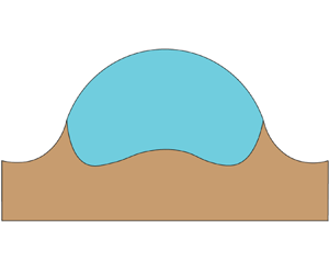
Consider a two-dimensional (2-D) liquid droplet in contact with a solid substrate that has a free surface at  $z=0$ and a rigid base pinned at $z=-\lambda$, as shown in figure 1. The drop undergoes spontaneous spreading of constant velocity $v$, as defined by contact-line radius $r(t)=r_o+vt$, where $r_o$ is the initial radius. This assumption of constant spreading rate is reasonable considering the relatively slow spreading rates found in soft wetting experiments (Carré, Gastel & Shanahan Reference Carré, Gastel and Shanahan1996; Van Gorcum et al. Reference Van Gorcum, Karpitschka, Andreotti and Snoeijer2020). The liquid–gas interface is located at $z=h(x,t)$ and forms the macroscopic contact angle $\theta (t)$ with the horizontal at the contact line, while the deformed solid–liquid interface is located at $z=w(x,t)$. We neglect the effect of gravity on the drop shape by considering the Bond number, $Bo=\rho g r_0^2/\gamma$ to be small in both liquid and solid, where $\rho$ is the material density and g is the gravitational acceleration. This means that the drop sizes we consider are below the capillary length scale. For example, in an experiment with glycerol ( $\rho _f=1260\ {\rm kg}\ {\rm m}^{-3}$, $\gamma _{lg}=0.064\ {\rm N}\ {\rm m}^{-1}$) drop on PDMS substrate ( $\rho _s=970\ {\rm kg}\ {\rm m}^{-3}$, $\gamma _{s}=0.02\ {\rm N}\ {\rm m}^{-1}$) the capillary length scale is between $1.5\sim 2\ {\rm mm}$.

Figure 1. Definition sketch.
2.1. Field equations
The spreading process is determined by the dynamic response of both the fluid flow and the solid deformation, as well as the interactions between the two. Here, the field equations for the fluid are defined in the current configuration, whereas the field equations for the solid are defined in the reference configuration, assuming small strains.
2.1.1. Fluid field
The flow field inside the spreading drop is described through a 2-D velocity field as  $\boldsymbol {v}=v_x(x,z)\boldsymbol {e}_x+v_z(x,z)\boldsymbol {e}_z$. The droplet is incompressible with a constant dynamic viscosity $\mu$ and has a stress tensor $\boldsymbol{\mathsf{T}}^f$ given by
 \begin{equation} T_{ij}^f=-P_f\delta_{ij}+\mu\left(\frac{\partial v_i}{\partial x_j}+\frac{\partial v_j}{\partial x_i}\right), \end{equation}
where  $P_f$ is the fluid pressure and $\delta$ is the Kronecker delta function. The velocity field obeys the momentum balance and incompressibility conditions
 $$\begin{gather} \rho_f\left(\frac{\partial \boldsymbol{v}}{\partial t}+\boldsymbol{v}\boldsymbol{\cdot}\boldsymbol{\nabla} \boldsymbol{v}\right)=-\boldsymbol{\nabla} P_f+\mu\nabla^2\boldsymbol{v}, \end{gather}$$
 $$\begin{gather}\boldsymbol{\nabla}\boldsymbol{\cdot}\boldsymbol{v}=0. \end{gather}$$
2.1.2. Solid field
The solid substrate is described by a 2-D deformation field  $\boldsymbol {u}=u_x(x,z)\boldsymbol {e}_x+u_z(x,z)\boldsymbol {e}_z$. We assume the material is incompressible and linear viscoelastic with time-dependent stress tensor given by (Christensen Reference Christensen2012)
 \begin{equation} T_{ij}^s=-P_s\delta_{ij}+G_o\psi\ast\left(\frac{\partial u_i}{\partial x_j}+\frac{\partial u_j}{\partial x_i}\right). \end{equation}
Here,  $\psi (t)$ is a relaxation function, $G_o$ the static shear modulus, $P_s$ the pressure in the solid and $f\ast g$ is a convolution operator defined as $f\ast g =\int _{-\infty }^t f(t-t'){\partial g}/{\partial t'}$. The functional form of $\psi (t)$ depends on the rheology of the solid. Typical examples include the well-known power-law model $\psi (t)=1+\varGamma (1-n)^{-1}(\tau /t)^n$, and the classical Kelvin–Voigt model $\psi =H(t)+\tau \delta (t)$ (Long et al. Reference Long, Ajdari and Leibler1996; Karpitschka et al. Reference Karpitschka, Das, van Gorcum, Perrin, Andreotti and Snoeijer2015). Here, $\tau$ is the relaxation time scale and $n$ is the power-law exponent, $\varGamma$ is the gamma function and $H$ is the Heaviside theta function. The 2-D nature of this formulation makes it similar to plane strain problems typically studied in solid mechanics.
The solid deformation field obeys the momentum balance and incompressibility equations
 $$\begin{gather} \rho_s \frac{\partial^2 \boldsymbol{u}}{\partial t^2}=-\boldsymbol{\nabla} P_s+G_o \psi\ast \nabla^2\boldsymbol{u}, \end{gather}$$
 $$\begin{gather}\boldsymbol{\nabla}\boldsymbol{\cdot}\boldsymbol{u}=0. \end{gather}$$
2.2. Boundary conditions
At the liquid–gas interface  $z=h(x,t)$, we apply a kinematic condition relating the fluid velocity to the interface velocity there, and balance the normal and shear stresses
 \begin{equation} v_z=\frac{\partial h}{\partial t}+v_x\frac{\partial h}{\partial x}, \quad \boldsymbol{n}\boldsymbol{\cdot}\boldsymbol{T}^f\boldsymbol{\cdot}\boldsymbol{n}=-\gamma_{lg}\kappa_f,\quad \boldsymbol{t}\boldsymbol{\cdot}\boldsymbol{T}^f\boldsymbol{\cdot}\boldsymbol{n}=0. \end{equation}
Here,  $\boldsymbol {n}$ and $\boldsymbol {t}$ are normal and tangential unit vectors along the interface, and $\kappa _f={\partial ^2h}/{\partial x^2}(1+({\partial h}/{\partial x})^2)^{-3/2}$ is the curvature.
At the liquid–solid interface, the field variables in the two domains interact and couple the two sets of governing equations. Here, we evaluate the solid deformation field in the reference configuration  $z=0$, and the fluid field in the current configuration $z=w(x,t)$, which are related through a kinematic condition $u_z(z=0)=w$. Continuity of velocity dictates the velocity field in the fluid to be equal to the rate of deformation in the solid
 $$\begin{gather} \left.v_x\right|_{z=w}=\left.\frac{\partial u_x}{\partial t}\right|_{z=0}+\left.\beta \frac{\partial v_x}{\partial z}\right|_{z=w}, \end{gather}$$
 $$\begin{gather}\left.v_z\right|_{z=w}=\left.\frac{\partial u_z}{\partial t}\right|_{z=0}+\left.\left(\frac{\partial u_x}{\partial t}\frac{\partial u_z}{\partial x}\right)\right|_{z=0}, \end{gather}$$
where  $\beta$ is the slip length introduced to relieve the stress singularity that may arise at the contact line. Stress continuity is given by
 $$\begin{gather} \boldsymbol{n}\boldsymbol{\cdot}\boldsymbol{T}^s\boldsymbol{\cdot}\boldsymbol{n}- \boldsymbol{n}\boldsymbol{\cdot}\boldsymbol{T}^f\boldsymbol{\cdot}\boldsymbol{n}=\gamma_s\kappa_s+ F_{cl}(x,t), \end{gather}$$
 $$\begin{gather}\boldsymbol{t}\boldsymbol{\cdot}\boldsymbol{T}^s\boldsymbol{\cdot}\boldsymbol{n}= \boldsymbol{t}\boldsymbol{\cdot}\boldsymbol{T}^f\boldsymbol{\cdot}\boldsymbol{n}, \end{gather}$$
where  $\kappa _s$ is the curvature of the solid free surface. The inclusion of the solid surface tension $\gamma _s$ in the normal stress condition (2.7a) regularizes the stress singularity at the contact point (Jerison et al. Reference Jerison, Xu, Wilen and Dufresne2011). By assuming a uniform $\gamma _s$ throughout the free surface we also neglect any difference between solid surface tension on the liquid and gas sides. The contact-line force $F_{cl}$ is given by
 \begin{equation} F_{cl}=\gamma_{lg}\sin \theta \delta(r(t)-|x|), \end{equation}
where  $\delta$ is the Dirac delta function. Here, $\theta$ is the macroscopic contact angle between the liquid interface and the horizontal axis. Note that we have ignored for simplicity the Laplace pressure inside the liquid which should be small in the limiting case of large drops. In our formulation, this limit is realized when the vertical thickness in both the liquid and solid domains is small compared with the drop radius, i.e. $\lambda /r_0,h/r_0\ll 1.$ This is consistent with the thin-film approximation to be considered in this work and also simplifies the analysis of viscoelastic spreading. This assumption can be relaxed for a purely elastic substrate whose rheology is time independent. We illustrate the potential effect of Laplace pressure for this limit in Appendix B and show that the spreading dynamics is nearly unaffected in the parameter ranges considered in this work. The macroscopic contact angle $\theta$ can be defined from the slope of the liquid–gas interface at the contact line
 \begin{equation} \tan \theta=\left.\frac{\partial h}{\partial x}\right|_{x=r(t)}. \end{equation}
Finally, we impose a no-displacement condition at the rigid base,
 \begin{equation} \boldsymbol{u}|_{z=-\lambda}=0. \end{equation}
 This is a free surface flow and the shape of the liquid–gas  $h(x,t)$ and solid $g(x,t)$ interfaces need to be determined as part of the solution. For this, we impose the following shape boundary conditions:
 $$\begin{gather} h(r(t),t)=w(r(t),t), \quad \text{: condition of contact} \end{gather}$$
 $$\begin{gather}\left. \frac{\partial h}{\partial x}\right|_{x=0}= \left.\frac{\partial w}{\partial x}\right|_{x=0}= \left.\frac{\partial^3 h}{\partial x^3}\right|_{x=0}= \left.\frac{\partial^3 w}{\partial x^3}\right|_{x=0}=0, \quad \text{: smoothness and symmetry} \end{gather}$$
 $$\begin{gather}\int_{-r(t)}^{+r(t)}(h-w)\,{{\rm d}\kern0.7pt x}=V_0, \quad \text{: volume conservation,} \end{gather}$$
where  $V_0$ is the equilibrium drop volume.
3. Lubrication approximation
We solve the coupled boundary value problem using the lubrication approximation (Oron et al. Reference Oron, Davis and Bankoff1997).
3.1. Scaling
We scale the horizontal and vertical lengths with  $r_o$ and $r_o\theta _o$, which are the initial drop radius and thickness, respectively. By considering the drop to be a thin film, we assume $\theta _o$ to be a small parameter, $\theta _o\ll 1$. We choose a characteristic velocity scale $\kappa \theta _0^p$, where $\kappa$ and $p$ are two experimental parameters related to the contact line speed (Ehrhard & Davis Reference Ehrhard and Davis1991; Smith Reference Smith1995). The scalings
 \begin{align} \left.\begin{gathered} x=x^*r_o,\quad z=z^*r_o \theta_o, \quad t=t^*r_o/\kappa \theta_0^p, \quad v_x^*=v_x\kappa \theta_0^p, \quad v_z^*=v_z\kappa \theta_0^{p+1}, \\ p_f=p_f^*\mu \kappa \theta_0^{p-2}/r_o, \quad u_x=u_x^*r_o, \quad u_z=u_z^*r_o\theta_o, \quad p_s=p_s^*\mu \kappa \theta_0^{p-2}/r_o, \quad \theta=\theta^*\theta_o, \end{gathered}\right\} \end{align}
are applied to the governing equations, which gives rise to the following dimensionless groups:
 \begin{align} C=\frac{\mu \kappa \theta_0^{p-3}}{\gamma_{lg}},\quad \sigma= \frac{\gamma_{lg}\theta_o^3}{G_o r_o},\quad\varepsilon=\frac{G_0\tau}{ \mu}, \quad\varPi=\frac{\gamma_{s}}{\gamma_{lg}}, \quad \varLambda=\frac{\lambda}{r_o\theta_o}, \quad \beta'=\frac{\beta}{r_o\theta_o}. \end{align}
Here,  $C$ is the viscocapillary number, $\sigma$ is the elastocapillary number and $\varepsilon$ is the relative viscosity of the substrate which includes the viscoelastic time scale $\tau$. Here $\varepsilon =0$ refers to a purely elastic substrate. Also, we define $\varPi$ as the surface tension ratio, $\varLambda$ as the solid aspect ratio, and $\beta '$ as the dimensionless slip length. We fix these parameters at $\varPi =2, \varLambda =0.5, \beta =0.01$, unless stated otherwise, and focus on the remaining parameters. As shown by Limat (Reference Limat2012), the ratio between liquid and solid surface tension needs to be small for the condition of linear elasticity to hold, and therefore we work with $\varPi >1$. The $\varLambda$ and $\beta$ values represent a thin substrate and a small slip length, respectively. It is known from previous works that increase of both substrate thickness and elasticity can increase the deformability of the solid and thus play a role in the wetting process (Zhao et al. Reference Zhao, Dervaux, Narita, Lequeux, Limat and Roché2018; Khattak et al. Reference Khattak, Karpitschka, Snoeijer and Dalnoki-Veress2022). Therefore, we typically fix the value of $\varLambda$ and focus on the effect of $\sigma$ only. The range of elastocapillary number where our reduced model will be valid is $\sigma \leqslant O(1)$ and this is the range where we report our results. If $\sigma$ is much higher, the bulk deformation in the substrate can become more significant than the deformation at the contact line and the thin film approximations on the stress condition at the solid–liquid boundary may break down. The subsequent sections have been written in dimensionless form and asterisks have been dropped hereafter.
3.2. Thin-film equations
Applying the lubrication approximation to the scaled boundary value problem and ignoring terms of  $O(\theta _o^2)$ gives rise to a reduced set of equations. The $x$ and $z$ components of the fluid (2.2a) and solid (2.4a) momentum balance equations become
 $$\begin{gather} -\frac{\partial P_f}{\partial x}+\frac{\partial^2 v_x}{\partial z^2}=0, \quad -\frac{\partial P_f}{\partial z}=0, \end{gather}$$
 $$\begin{gather}-C\sigma\frac{\partial P_s}{\partial x}+\psi \ast \frac{\partial^2 u_x}{\partial z^2}=0,\quad \frac{\partial P_s}{\partial z}=0. \end{gather}$$
The incompressibility conditions (2.2b), (2.4b) remain invariant under the lubrication approximation. The boundary conditions (2.5)–(2.10) become
 $$\begin{gather} Cp_f|_{z=h}=-\frac{\partial^2~h}{\partial x^2}, \quad \left.\frac{\partial v_x}{\partial z}\right|_{z=h}=0, \quad v_z|_{z=h}=\frac{\partial h}{\partial t}+\frac{\partial h}{\partial x}v_x|_{z=h}, \end{gather}$$
 $$\begin{gather}-C P_s|_{z=0}+C P_f|_{z=w}=\left.\varPi\frac{\partial^2 u_z}{\partial x^2} \right|_{z=0}+\sigma\bar{F}_{cl}, \end{gather}$$
 $$\begin{gather}\left.\psi \ast \frac{\partial u_x}{\partial z}\right|_{z=0}=C\sigma \left.\frac{\partial v_x}{\partial z}\right|_{z=w}, \end{gather}$$
 $$\begin{gather}\left.v_x\right|_{z=w}=\left.\frac{\partial u_x}{\partial t}\right|_{z=0}+\beta' \left.\frac{\partial v_x}{\partial z}\right|_{z=w}, \quad \left.v_z\right|_{z=w}= \left.\frac{\partial u_z}{\partial t}\right|_{z=0}+\left.\left(\frac{\partial u_x}{\partial t} \frac{\partial u_z}{\partial x}\right)\right|_{z=0}, \end{gather}$$
 $$\begin{gather}u_x|_{z=-\varLambda}=u_z|_{z=-\varLambda}=0. \end{gather}$$
Here,  $\bar {F}_{cl}=\theta \delta (r(t)-|x|)$ is the dimensionless contact-line force, with the contact angle
 \begin{equation} \theta=\left.\frac{\partial h}{\partial x}\right|_{x=r(t)}. \end{equation}
The dimensionless forms of the shape boundary conditions (2.11) are given by
 \begin{equation} h(r(t),t)=w(r(t),t), \quad \left.\frac{\partial h}{\partial x}\right|_{x=0}=\left.\frac{\partial^3 h}{\partial x^3}\right|_{x=0}=0, \quad \int_{-r(t)}^{+r(t)}(h-w)\,{{\rm d}\kern0.7pt x}=1, \end{equation}
which illustrate the coupling between the fluid and solid domains.
4. Solution method
We begin by deriving evolution equations for the liquid-gas interface  $h$ and the solid interface $w$, which we then expand in the small viscocapillary number $C$ limit to facilitate a solution.
4.1. Fluid flow
In the fluid domain, we begin by integrating (3.3a,b) with respect to  $z$ and applying the pressure and velocity boundary conditions (3.4a,b,f) to determine the pressure $p$ and horizontal velocity field $v_x$. We then use the continuity equation (2.2b) to determine the vertical velocity field $v_z$. The velocity and pressure fields are given by
 \begin{align} Cv_x &=\frac{\partial^3 h}{\partial x^3}\left(hz-hw-\frac{z^2}{2}+\frac{w^2}{2}+\beta'(h-w)\right)+C\left.\frac{\partial u_x}{\partial t}\right|_{z=0}, \end{align}
 \begin{align} Cv_z&=\frac{\partial^4 h}{\partial x^4}\left(hw-\frac{1}{2}\left(hz+w^2\right)+\frac{1}{6}\left(z^2+zw+w^2\right)\right) (z-w)\nonumber\\ &\quad+\frac{\partial^3 h}{\partial x^3}\left(\frac{\partial w}{\partial x}(h-w)-\frac{1}{2}\frac{\partial h}{\partial x} (z-w)-\beta'\left(\frac{\partial h}{\partial x}-\frac{\partial w}{\partial x}\right)\right)\nonumber\\ &\qquad C\left(\left. (z-w)\frac{\partial^2u_x}{\partial x \partial t}\right|_{z=0}+ \frac{\partial w}{\partial t}+\left.\frac{\partial w}{\partial x}\frac{\partial u_x}{\partial t}\right|_{z=0}\right), \end{align}
 \begin{align} Cp &=-\frac{\partial^2h}{\partial x^2}. \end{align}
Integrating (2.2b) from  $h(x,t)$ to $w(x,t)$ and applying the appropriate boundary conditions gives a depth averaged continuity equation,
 \begin{equation} \frac{\partial}{\partial t}(h-w)+\frac{\partial}{\partial x}\int_w^h v_x \,{\rm d}z=0, \end{equation}
which, when we apply (4.1a), gives the first evolution equation
 \begin{equation} C\frac{\partial}{\partial t} (h-w) +\frac{\partial}{\partial x}\left[\frac{\partial^3 h}{\partial x^3}\left(\frac{1}{3}(h-w)^3+\beta'(h-w)^2\right)+C\left.\frac{\partial u_x}{\partial t}\right|_{z=0}(h-w)\right]=0. \end{equation}
4.2. Solid deformation
The second evolution equation is determined from the thin-film equations in the solid domain (3.3c,d), (2.4b) with boundary conditions at the solid surface and the rigid base (3.4d), (3.4e), (3.4h,i). A closed form solution for the deformation field components can be determined as
 \begin{align} \psi\ast u_x &=\sigma\left(\frac{\varPi}{2}\frac{\partial^3 w}{\partial x^3}+\frac{\partial^3 h}{\partial x^3}- \frac{1}{2}\frac{\partial}{\partial x}\bar{F}_{cl}\right)(\varLambda^2-z^2)+C\sigma \frac{\partial^3 h}{\partial x^3}(h-w) (z+\varLambda),\end{align}
 \begin{align} \psi\ast u_z&=\sigma\left(\frac{\varPi}{2}\frac{\partial^4 w}{\partial x^4}+\frac{\partial^4 h}{\partial x^4}+ \frac{1}{2}\frac{\partial^2}{\partial x^2}\bar{F}_{cl}\right)\left(\frac{z^3}{3}-\varLambda^2z- \frac{2\varLambda^3}{3}\right)\nonumber\\ & \quad -C\sigma\frac{\partial^4 h}{\partial x^4}(h-w)\left(\frac{z^2}{2}+\varLambda z+\frac{\varLambda^2}{2}\right), \end{align}
which, when evaluated at  $z=0$, gives the desired evolution equation at the solid interface
 \begin{equation} \psi\ast w=-\frac{\sigma\varLambda^3}{3}\left(\varPi\frac{\partial^4 w}{\partial x^4}+2\frac{\partial^4 h}{\partial x^4}+\frac{\partial^2}{\partial x^2}\bar{F}_{cl}\right)-\frac{C\sigma\varLambda^2}{2}\frac{\partial^4 h}{\partial x^4}(h-w)(z+\varLambda). \end{equation}
 Equations (4.3) and (4.5) need to be solved simultaneously, with the associated shape boundary conditions (2.11), to determine the unknown functions  $h(x,t)$ and $w(x,t)$.
4.3. The small  $C$ limit

Droplet spreading in the viscosity-dominated regime is typically a slow dynamic process such that the characteristic velocity can be of the order of microns/second. Therefore, we can assume the viscocapillary number to be a small parameter, i.e.  $C\ll 1$, and expand the unknown functions in $C$ as
 \begin{equation} h=h_o+Ch_1, \quad w=w_o+Cw_1, \quad u_x=u_x^0+Cu_x^1, \quad \theta=\theta_o+C\theta_1. \end{equation}
4.3.1. Leading-order solution
At  $O(1)$ the fluid evolution equation (4.3) reduces to a steady state condition without explicit time dependence. The leading-order liquid–gas interface shape $h_o(x,t)$ only implicitly depends on time through the contact-line position $r(t)$. The liquid–gas interface shape at this order is quasi-steady and independent of slip
 \begin{equation} \frac{\partial^3h_o}{\partial x^3}=0, \end{equation}
with shape boundary conditions (3.6a–c) given by
 \begin{equation} h_o(r(t))=w_o(r(t)), \quad \left.\frac{\partial h_o}{\partial x}\right|_{x=0}=0, \quad \int_{-r(t)}^{+r(t)}(h_o-w_o)\,{\rm d}\kern0.7pt x=1. \end{equation}
The leading-order solid deformation  $w_o$ can be obtained from the reduced form of (4.5)
 \begin{equation} \psi\ast w_o+\frac{\sigma\varLambda^3}{3}\left(\varPi\frac{\partial^4w_o}{\partial x^4}+\frac{\partial^2}{\partial x^2} \bar{F}_{cl}\right)=0.\end{equation}
Equation (4.9) is a partial integro-differential equation when the substrate response is viscoelastic. To solve this equation we assume a constant spreading velocity,  $V$ such that $r(t)=1+Vt$ and use the Fourier transform method. We employ a double Fourier transform to convert variables $t$ and $x$ into frequency $\omega$ and wavenumber $s$, respectively, using the following integral transformation pair (Sneddon Reference Sneddon1995):
 $$\begin{gather} \hat{\tilde{f}}(s,\omega)=\frac{1}{2{\rm \pi}}\iint_{-\infty}^{\infty}f(x,t) \exp({{\rm i}(sx+\omega t)})\,{\rm d}\kern0.7pt x\,{\rm d}t, \end{gather}$$
 $$\begin{gather}f(x,t)=\frac{1}{2{\rm \pi}}\iint_{-\infty}^{\infty}\hat{\tilde{f}}(s,\omega) \exp({-{\rm i}(sx+\omega t)})\,{\rm d}s\,{\rm d}\omega. \end{gather}$$
Here, the wavenumber and frequency are made dimensionless by scaling them with the horizontal length and time scales of the system, respectively. In this transformed space, (4.9) becomes an algebraic equation for  $\hat {\tilde {w}}_o$ that can be solved
 \begin{equation} \hat{\tilde{w}}_o=\frac{\sigma \varLambda^3 s^2 \hat{\tilde{F}}_{cl}(s,\omega)}{\varPi \sigma \varLambda^3 s^4+3\tilde{\psi}(\omega)}, \end{equation}
where  $\hat {\tilde {F}}_{cl}(s,\omega )=\bar {\theta }(\textrm {e}^{\textrm {i}s}\delta (\omega +sV)+\textrm {e}^{-\textrm {i}s}\delta (\omega -sV))$ with $\bar {\theta }={\partial h_o}/{\partial x}|_{x=r(t)}$, and $\tilde {\psi }(\omega )$ is a frequency dependent shear modulus.
The inverse Fourier transform of (4.11) into the time domain is easily resolved by using the following property of the Dirac delta function:
 \begin{equation} \int_{-\infty}^{\infty}f(\omega)\delta(\omega-\omega_o)\,{\rm d}\omega=f(\omega_o). \end{equation}
Finally, the transformation back into the spatial domain can be achieved by numerical integration of
 \begin{align} w_o(x,t)=\frac{1}{\sqrt{2{\rm \pi}}}\int_{-\infty}^{\infty}\sigma\varLambda^3s^2\left(\frac{ \exp({{\rm i}s(1+vt)})}{3\hat{\psi}(-sV)+\varPi\sigma\varLambda^3s^4} + \frac{\exp({-{\rm i}s(1+vt)})}{3\hat{\psi}(sV)+\varPi\sigma\varLambda^3s^4}\right){\rm d}s. \end{align}
To find the interface shapes during the spreading motion, we numerically solve (4.13) and (4.7) with the shape boundary conditions using a finite difference scheme. Note that, for a purely elastic substrate, the convolution operator in (4.5) is simply a constant and the transformation in the time domain is not required. For this special case, we can solve for an arbitrary contact-line position  $r(t)$ which needs to be described from a constitutive equation. We describe this limiting case in detail in § 5.3.
4.3.2. First-order solution
Next, we solve the  $O(C)$ fluid (4.3) and solid (4.5) evolution equations
 $$\begin{gather} \frac{\partial}{\partial t}(h_o-w_o)+\frac{\partial}{\partial x}\left(\frac{\partial^3 h_1}{\partial x^3}\left(\frac{1}{3}(h_o-w_o)^3+\beta'(h_o-w_o)^2\right) \left.+\frac{\partial u_{x}^o}{\partial t}\right|_{z=0}(h_o-w_o)\right)=0, \end{gather}$$
 $$\begin{gather}\psi\ast w_1+\frac{\sigma\varLambda^3}{3} \left(\varPi\frac{\partial^4 w_1}{\partial x^4}+\frac{\partial^4 h_1}{\partial x^4}\right)=0, \end{gather}$$
with the  $O(C)$ shape boundary conditions
 \begin{equation} \left.\begin{gathered} h_1(r(t))=w_1(r(t))=0, \quad \int_{-r(t)}^{+r(t)}(h_1-w_1)\,{{\rm d}\kern0.7pt x}=0, \\ \frac{\partial h_1}{\partial x}=\frac{\partial w_1}{\partial x}=\frac{\partial^3 h_1}{\partial x^3}=\frac{\partial^3 w_1}{\partial x^3}=0 \quad \text{at $x=0$.} \end{gathered}\right\} \end{equation}
The integro-differential equation (4.14b) can be greatly simplified by considering only the leading-order contribution to the viscoelastic relaxation. Carré & Shanahan (Reference Carré and Shanahan1995) and Shanahan (Reference Shanahan1988) have shown that the wetting ridge on a viscoelastic substrate can act as a dissipative sink which largely controls the spreading dynamics. Since the contact-line forces responsible for creating the wetting ridge do not appear at  $O(C)$, we can assume viscoelastic effects at this order to be trivial and approximate the first term in (4.14b) as $\psi \ast w_1\approx w_1$. This allows us to compute the solution of (4.1a,b) as a system of ordinary differential equations, thereby reducing the computational loads significantly. Details of the numerical algorithm used are given in Appendix A.
4.3.3. Rheology
We have formulated the problem in a way that any known rheology of linear viscoelasticity described with a single time scale can be replaced in  $\tilde {\psi }(\omega )$ and the corresponding interface shapes can be found using the methods outlined above. For the results reported in the following section, we make use of the power-law rheology given by
 \begin{equation} \tilde{\psi}(\omega)=1+({\rm i}\omega\eta)^n, \end{equation}
with  $\eta =\varepsilon \sigma C$. This is a generalization of the classic Kelvin–Voigt model ( $n=1$), and is relevant for PDMS substrates. It is also straightforward to generalize to other rheologies.
5. Results
Here, we report the results from the two-way coupled model of viscous drop spreading on a deformable substrate. Our focus is on how the dimensionless material parameters, e.g.  $\sigma,\varLambda, \varepsilon, C$ affect the spreading dynamics. Here, we show how substrate elasticity and viscosity affect the interface shapes $h(x,t),w(x,t)$, and subsequently the dynamic contact angle $\theta$ and the related flow fields for given spreading velocity $V$. Then, through a power balance analysis, we show how the spontaneous contact-line velocity $V$ can be estimated as a function of $\theta$ in different regimes. Next, we consider the purely elastic limit $\varepsilon =0$ of the rheology (4.16) and compare the spreading rate on a deformable substrate with the well-known Tanner's law for drop spreading on a rigid substrate.
5.1. Spreading on a viscoelastic substrate
Figure 2 plots the dynamic liquid–gas and liquid–solid interfaces for a viscous droplet spreading on a viscoelastic substrate with a constant contact-line velocity. Figure 2(a) shows that as time  $t$ increases the droplet width increases and the height decreases, because of the positive spreading velocity $V$. The maximum substrate deformation occurs at the contact line and similarly decreases with time due to solid viscoelastic dissipation. Figure 2(b) shows the effect of solid elasticity on the interface shape where increasing elastocapillary number $\sigma$ corresponds to a more deformable substrate. Here, increases in $\sigma$ correspond to increases in the wetting ridge height, as well as the overall deformation in the bulk of the solid with a corresponding decrease in the contact angle on soft substrates. These results reveal a contrasting role of solid viscous dissipation and elastic resistance on the shape of the interface.

Figure 2. Liquid and solid interface shapes during spreading, as they depend upon the (a) time  $t$ for fixed elastocapillary number $\sigma =0.5$, and (b) elastocapillary number $\sigma$ for fixed time $t=1$. Here, $C=0.2, \varepsilon =2, n=1, V=0.1$.
The macroscopic contact angle  $\theta$ is a key parameter to characterize the spreading dynamics of a moving contact line. This angle is determined by measuring the slope of the liquid–gas interface at the contact point using (3.5). Figure 3(a) illustrates the dependence of the contact angle $\theta$ on the dimensionless time $t$, for different spreading velocities $V$. This shows that $\theta$ remains nearly constant with respect to time $t$ for small velocity $V=0.01$, but becomes a decreasing function of time for higher velocities, e.g. $V=0.2$. Note that the velocity $V$ is considered to be a free parameter in this solution and here we observe how the contact angle, and therefore the drop shape, changes over time as the contact line travels at different speeds. The decrease in contact angle occurs due to the volume conservation in the droplet. Figure 3(b,c) plots $\theta$ against $V$ as it depends upon ( $b$) the viscosity ratio $\varepsilon$ and ( $c$) elastocapillary number $\sigma$, to illustrate the contrasting effects of substrate viscosity and elasticity. In figure 3(b) we find that increasing $\varepsilon$ also increases $\theta$ for a fixed velocity. This implies that, on a substrate with higher viscous dissipation, it will take longer to reach an equilibrium state and the spreading motion will be slowed, consistent with previous experimental observations (Shanahan & Carre Reference Shanahan and Carre1995; Chen, Bonaccurso & Shanahan Reference Chen, Bonaccurso and Shanahan2013). Figure 3(c) plots $\theta$ against velocity $V$ as it depends upon the elastocapillary number $\sigma$, showing $\theta$ decreases with increasing $V$ and these trends also decrease with increasing $\sigma$ or substrate softness. This means that, for a given droplet shape, i.e. a given $\theta$, the spreading velocity $V$ will be higher on softer substrates, as opposed to the smaller velocities found in more viscoelastic substrates.

Figure 3. Contact angle  $\theta$ against (a) time $t$, as it depends upon contact-line velocity $V$ (
$V$ ( $\sigma =0.5, \varepsilon =5$), and against (b,c) velocity $V$, as it depends upon the (b) viscosity ratio $\varepsilon$ ( $t=1, \sigma =0.5$) and the (c) elastocapillary number $\sigma$ ( $\varepsilon =1, t=1$). For all panels, $C=0.2, n=0.6.$
Figure 4 plots typical flow fields. Figure 4(a) shows the limiting case of liquid spreading on a rigid substrate  $\sigma =0, \varepsilon =0$, where the fluid motion is directed from the bulk towards the contact line, which results in an increased drop radius and reduced height. On a soft substrate, the internal flow can be more complex due to the deformability of the substrate and this will affect the spreading dynamics. This is illustrated in figure 4(b), which plots the flow field for a drop on a highly viscoelastic substrate with $\sigma =0.2, \varepsilon =50$ with wetting ridge formed at the contact line and neighbouring depression of the substrate. Here, some fluid inside the droplet moves towards the depressed region creating a recirculation flow that causes less fluid to move towards the contact line. This so-called ‘dissipative sink’ prevents contact-line motion and results in reduced spreading (Carré & Shanahan Reference Carré and Shanahan1995). For a moderately viscoelastic substrate ( $\varepsilon =1, \sigma =0.2$), figure 4(c) shows the deformation increases away from the contact line and the ‘dissipative sink’ becomes less sharp. Here, the recirculation flow has moved away from the contact-line region and more fluid is being directed towards the centre of the drop. This is an intermediate regime where, in addition to the flow towards the dissipative sink, some of the fluid also moves downwards pushing the bulk of the droplet onto the solid substrate. This occurs because substrate deformability increases with reduced viscoelastic dissipation $\varepsilon$ and solid deformability is favourable to contact angle reduction. Since $\varepsilon$ and $\sigma$ are of similar magnitude in this case, the spreading dynamics is expected to be governed by a competition between the solid elasticity and solid viscosity. Figure 4(d) shows the flow field for a weakly viscoelastic substrate ( $\sigma =0.5, \varepsilon =0.1$), i.e. an elasticity-dominated case. Here, we find that the fluid flow is now directed primarily downwards and deforms the bulk substrate away from the contact line, which tends to decrease the contact angle and should result in an enhanced spreading rate. Therefore, we can conclude that the effect of solid elasticity is to enhance spreading, while viscosity inhibits spreading.

Figure 4. Flow fields on a (a) rigid  $\sigma =0,\varepsilon =0$, (b) highly viscoelastic $\sigma =0.1,\varepsilon =50$, (c) moderately viscoelastic $\sigma =0.1,\varepsilon =1$ and (d) nearly elastic $\sigma =0.5,\varepsilon =0.1$ substrate, with all other parameters fixed as $C=0.2, n=0.6, V=0.2, t=0.1$.
5.2. Estimating velocity from power balance
So far, the contact-line velocity  $V$ has been taken to be a free parameter, and the spreading dynamics associated with a given velocity has been studied. In the absence of external forcing, this velocity of spontaneous spreading in a droplet can be determined by considering the energy conservation of the system and combining it with the interface deformation model. This is done by considering the power balance between the driving force of capillarity and the rate of energy dissipation in the system, which can be expressed as
 \begin{equation} \mathcal{P}_f+\mathcal{P}_s=\gamma_{lg}\left(\cos \theta_e-\cos \theta\right)V, \end{equation}
where  $\mathcal {P}_f$ and $\mathcal {P}_s$ are the dissipated powers per unit depth in the fluid and solid, respectively. Here, $\theta _e$ is the equilibrium contact angle that depends on the substrate wettability and $\theta _e=0$ denotes complete wetting. For a thin film with small contact angle, we can approximate $\cos \theta _e-\cos \theta \approx (\theta ^2-\theta _e^2)/2$. Within the lubrication approximation, the power balance can be expressed as
 \begin{equation} \int_{-\infty}^{\infty}{\rm d}\kern0.7pt x\left(C \sigma \int_0^h {\rm d}z \left(\frac{\partial v_x}{\partial z}\right)^2+\int_{-\varLambda}^0 \psi \ast \frac{\partial ^2 u_x}{\partial t \partial z} \frac{\partial u_x}{\partial z} {\rm d}z\right)=\frac{1}{2}\sigma V (\theta^2-\theta_e^2). \end{equation}
We can estimate the viscoelastic dissipation in a thin solid substrate following an approach similar to Long et al. (Reference Long, Ajdari and Leibler1996). Briefly, we express the integral for  $P_s$ by using a Fourier transform into the frequency domain and then use Plancherel's theorem to convert the horizontal coordinate $x$ into wavenumber $s$ to get
 \begin{equation} \mathcal{P}_s=\int_{-\infty}^{\infty}{\rm d}s \int_{-\varLambda}^0{\rm d}z sV(s\eta V)^n\left(\frac{\partial \hat{u}_x (s,z)}{\partial z} \right)^2. \end{equation}
From the horizontal deformation equation (4.4a), we can determine the scale of the horizontal shear stress as  $\partial \hat {u}_x/\partial z \approx \sigma z/s$. The integral over the $s$ domain would then diverge at $s=\infty$ and lead to infinite viscoelastic dissipation. Including solid surface tension in the solid deformation model regularizes this singularity and provides a cutoff wavenumber $s_{max}=\epsilon$ (Jerison et al. Reference Jerison, Xu, Wilen and Dufresne2011). Through numerical tests (illustrated in Appendix C), we typically find $\epsilon =O(10)$.
To determine the scale of the fluid dissipation, one can assume Poiseuille flow in the drop as  $\partial v_z/\partial z\approx Vz/h^2$. Then, we can simplify (5.2) as
 \begin{align} \int_{x_{min}}^{x_{max}}{\rm d}\kern0.7pt x \int_0^h {\rm d}z C\left(\frac{Vz}{h^2}\right)^2 +\int_0^{\epsilon}{\rm d}s \int_{-\varLambda}^0 {\rm d}z \sigma^{n+1} (\varepsilon C)^n V^{n+1} s^{n-1} z^2\approx \frac{1}{2} V(\theta^2-\theta_e^2). \end{align}
Using (5.4) one can determine the relationship between contact angle  $\theta$ and velocity $V$ in a system where both solid and liquid dissipations are important. Two important limiting cases can be recovered from this nonlinear equation. For complete spreading on a rigid surface ( $\theta _e=0, \varepsilon =0$), the driving capillary force is balanced only by the fluid dissipation. In this case, (5.4) can be solved to generate the following explicit relationship between the spreading velocity $V$ and contact angle $\theta$
 \begin{equation} CV\approx\frac{1}{\ell}\theta^3. \end{equation}
Here,  $\ell$ is a ratio of cutoff length scales in the droplet, which is typically $\ell =O(10)$ (De Gennes Reference de Gennes1985). Equation (5.5) is a reduced form of the general Cox–Voinov law for infinite spreading (Voinov Reference Voinov1976; Cox Reference Cox1986). The other limiting case is found when the viscoelastic dissipation dominates ( $\varepsilon \rightarrow \infty, C\rightarrow 0$) and balances the driving capillary force. In this case, we can write (5.4) as
 \begin{equation} (\sigma^{n+1} \varLambda^3)^{1/n}\varepsilon CV\approx\frac{1}{\epsilon}\theta^{2/n}. \end{equation}
This recovers the scaling relation between  $V$ and $\theta$ in the viscoelasticity-dominated regime when the thin-film limit is applied (Zhao et al. Reference Zhao, Dervaux, Narita, Lequeux, Limat and Roché2018). Carré & Shanahan (Reference Carré and Shanahan1995) have experimentally shown this scaling law to hold for fluids of different viscosities when the solid dissipation dominates the power balance. Here, we have identified a slow velocity scale in the viscoelasticity-dominated regime that depends upon the viscoelastic power-law exponent in the solid and can be directly compared with the velocity scale in the rigid case from (5.5). Zhao et al. (Reference Zhao, Dervaux, Narita, Lequeux, Limat and Roché2018) have also developed a similar scaling law from viscoelastic dissipation. In the intermediate regime of $0<\varepsilon <\infty$, the integral in (5.4) can be solved to find the more general relationship in the complete wetting case
 \begin{equation} CV\ell/\theta+\sigma^{n+1}(V\varepsilon C)^n\varLambda^3\epsilon^n\approx\theta^2/2, \end{equation}
which includes energy dissipation in both solid and liquid domains.
5.3. The limit of a purely elastic substrate
The effect of substrate softness on droplet spreading can be further investigated in the purely elastic limit  $\varepsilon =0$. Here, our focus is on the role of substrate deformability on spreading laws, i.e. variation of $r(t)$ as a power-law function of time $t$, which will be contrasted with the well-known Tanner's law for spreading on a rigid substrate (Tanner Reference Tanner1979). To do this, we relax the condition of constant spreading velocity and allow for a general spreading rate $\dot {r}(t)$. This requires one to prescribe a constitutive relationship for the contact-line speed. Here, we use the following empirical relationship written in dimensionless form which relates the contact angle $\theta$ to the contact-line speed $\dot {r}(t)$ (Dussan Reference Dussan1979; Ehrhard Reference Ehrhard1993):
 \begin{equation} \frac{{\rm d}r}{{\rm d}t}= (\theta-\theta_e)^p. \end{equation}
Here,  $\theta _e$ is the static contact angle whose value depends on the substrate wettability. The value of $p=3$ has been suggested in many previous studies (Schwartz & Tejada Reference Schwartz and Tejada1972; Tanner Reference Tanner1979), and this is the value we use here. Here, in the absence of viscoelastic dissipation, we have a constant relaxation function $\psi (\omega )=1$ and find the leading-order solid deformation from the following inverse spatial Fourier transform:
 \begin{equation} w_o(x,t)=\frac{1}{\sqrt{2{\rm \pi}}}\int_{-\infty}^{\infty}\frac{\sigma \varLambda^3 s^2 \hat{F}_{cl}}{\varPi \sigma \varLambda^3 s^4+3}{\rm e}^{-{\rm i}sx}\,{\rm d}s, \end{equation}
with  $\hat {F}_{cl}=\sqrt {2/{\rm \pi} }\theta \cos (s r(t))$ and $\theta >\theta _e$. The solution method outlined in the previous sections can be used to determine liquid interface shape $h(x,t)$, which can then be applied to the following dynamic contact-line condition:
 \begin{equation} \frac{{\rm d}r}{{\rm d}t}=\left(\left.\frac{\partial h}{\partial x}\right|_{x=r(t)}-\theta_e\right)^p. \end{equation}
 The drop will spread until the condition  $\theta >\theta _e$ is met, from which we can determine an equilibrium drop radius $R_{\infty }$ as $\textrm {d}r/\textrm {d}t|_{r=R_{\infty }}=0$. The dependence of $R_{\infty }$ on the substrate elasticity for the complete wetting case $\theta _e=0$ is shown in figure 5 which plots $R_{\infty }$ against the elastocapillary number $\sigma$ for different substrate thicknesses $\varLambda$. This shows that the equilibrium radius $R_{\infty }$ decreases with increased elastocapillary number $\sigma$ or substrate deformability. This is in agreement with figure 4, where we found that, during spreading on a soft substrate, the primary fluid flow is directed downwards, causing the contact angle to decrease and causing the drop to reach its equilibrium shape with a smaller radius. Note here that increasing the substrate thickness $\varLambda$ makes the substrate even more deformable, and thus also reduces $R_{\infty }$.

Figure 5. Equilibrium radius  $R_\infty$ on a purely elastic substrate $\varepsilon =0$, as it depends upon the elastocapillary number $\sigma$ and substrate thickness $\varLambda$, for $\theta _e=0$.
The approach to equilibrium can be determined by numerically solving (5.10) with initial condition  $r(0)=1$ using the forward Euler method. Here, we use an adaptive timestep and a maximum relative error of $10^{-6}$. Figure 6 plots the ( $a$) contact-line radius $r$ and ( $b$) contact angle against time. At long times, the dynamics approaches the power-law form $t^{\alpha }$ with characteristic exponent $\alpha$. In the rigid solid limit $\sigma =0$, we find an exponent $\alpha =0.1428$ that recovers the classic Tanner's law (Tanner Reference Tanner1979). Increasing the substrate deformability $\sigma$ causes the spreading rate to increase. For $\sigma =0.1$ and $\sigma =1$ we find the spreading-law exponent $\alpha$ to be $0.148$ and $0.153$, respectively. Figure 6 plots the corresponding contact angles $\theta (t)$ for the same parameter values as figure 6. To summarize, the effect of substrate deformability is to decrease the equilibrium radius $R_\infty$ and increase the spreading exponent $\alpha$.

Figure 6. Spreading on a purely elastic  $\varepsilon =0$ substrate plotting the (a) contact-line radius $r$ and (b) contact angle $\theta$ against time, as it depends upon the elastocapillary number $\sigma$ for $\theta _e=0$, exhibits a power-law $\sim t^{\alpha }$ for large times with exponent $\alpha$.
6. Concluding remarks
We have developed a theoretical model of a 2-D liquid drop spreading on a soft viscoelastic solid of arbitrary rheology using lubrication theory. The spreading dynamics is characterized by the dynamic liquid–gas and solid–liquid interface shapes and the macroscopic contact angle formed at the three-phase contact line, as the system approaches static equilibrium. On a deformable substrate, energy dissipation in both the liquid and solid affect the contact angle and determine the spreading rate. We find that, when the dissipation in the solid is larger than that in the liquid, the spreading rate is decreased through the internal flow fields. In contrast, increased substrate deformability or softness tends to enhance spreading, as the larger deformation tends to reduce the contact angle. Through a power balance argument, we identify a general relationship between spreading velocity and contact angle and also recover the appropriate limiting cases in the liquid-dominated dissipation and solid-dominated dissipation regimes. The effect of substrate elasticity is described in further detail in the limiting case of a purely elastic substrate, where we find a final equilibrium drop radius that becomes smaller as the solid becomes softer, which is accompanied by a faster spreading rate when compared with the well-known Tanner's law for droplet spreading on a rigid substrate.
Our work uncovers some essential features of this two-way coupled problem of a viscous fluid interacting with a soft viscoelastic solid. Here, we were able to study the most general problem where the liquid and solid viscosities are of comparable magnitude, and reveal the contrasting roles of solid viscosity and elasticity on the spreading dynamics. Our focus was on comparing spreading laws on soft substrates with rigid substrates in the complete wetting case, and an important extension of the current model would be to introduce the effect of partial wetting on the solid deformation field. For example, Charitatos & Kumar (Reference Charitatos and Kumar2020) have previously shown that when the equilibrium contact angle  $\theta _e>0$, the spreading rate can become slower on softer substrates due to the presence of an attractive van der Waals force. In addition, it is known in rigid wetting dynamics that the axisymmetric spreading rate of a 3-D drop scales as $r\sim t^{1/10}$, which is slower than the 2-D case of $r\sim t^{1/7}$, and developing a 3-D counterpart of the current model would provide key insights into the 3-D spreading dynamics.
In this work, we assume soft solids to be incompressible and that is typically valid for most materials used in experiment, such as PDMS (Karpitschka et al. Reference Karpitschka, Das, van Gorcum, Perrin, Andreotti and Snoeijer2015). But this need not always be the case. The current formulation can be extended to a finitely compressible material using a Galerkin vector formulation of deformation field  $\boldsymbol {u}$ (Tamim & Bostwick Reference Tamim and Bostwick2021a). Also, our 2-D formulation of spontaneous spreading should be easily extendible to more complex cases of soft wetting, such as droplet translation under a substrate gradient, or on an inclined surface. It has been shown in previous works that substrate wettability can play a non-trivial role in such phenomena (Bueno et al. Reference Bueno, Casquero, Bazilevs and Gomez2018), and the inclusion of the full effect of substrate wettability would be an important modification of the current model.
Lastly, our model can be used as an essential tool for validating novel experiments on soft wetting phenomena, such as dewetting of contact lines during dip-coating phenomenon (Kajiya et al. Reference Kajiya, Brunet, Royon, Daerr, Receveur and Limat2014; Bertin et al. Reference Bertin, Snoeijer, Raphaël and Salez2022). Numerical simulation of the fully 3-D two-way coupled elastocapillary wetting phenomena would also benefit from using this model as a benchmarking tool (Aland & Mokbel Reference Aland and Mokbel2021). Finally, this model can be useful in developing a general universal model of spreading on complex surfaces with arbitrary rheology and deformability.
Funding
J.B.B. acknowledges support from NSF Grant CBET-1750208.
Declaration of interests
The authors report no conflict of interest.
Appendix A. Numerical method for the evolution equations
To solve the  $O(1)$ evolution equation (4.7), we discretize the interface into a number of nodes and employ a first-order accurate forward finite difference scheme to express the derivatives. The integral boundary condition (4.8a–c) is defined using a standard Simpson's method. Here, using 50 nodes was typically enough to achieve convergence of the contact angle to $10^{-4}$. For the $O(C)$ evolution equation (4.14a), we are required to compute the time derivative term from the leading-order solutions $h_0$ and $w_0$, and to evaluate $\partial h_0/\partial t$ we integrate (4.7) twice using the boundary conditions (4.8a–c) to derive an expression for $h_0$ as
 \begin{equation} h_0=\frac{3}{4r^3}(r^2-x^2)\left(1-2rg_0+2\int_0^rg_0(x)\,{{\rm d}\kern0.7pt x}\right). \end{equation}
Here, we compute the time derivative by using  $r(t)=1+Vt$. For slow velocities $V\ll 1$, typically 50 nodes is sufficient to achieve a converged solid interface shape.
Appendix B. Effect of capillary pressure
The contribution of capillary pressure from the droplet onto the solid substrate has been suppressed thus far for simplicity of analysis. One can include capillary pressure into the model by redefining
 \begin{equation} F_{cl}=\gamma_{lg} \sin \theta \left(\delta (r(t)-|x|)-\frac{1}{r(t)}H(r(t)-|x|)\right), \end{equation}
with  $H$ the Heaviside theta function, and investigate the effect in the purely elastic limit $\varepsilon =0$. Figure 7(a) plots the interface shapes for $\sigma =1, r=1.5$, contrasting the effect of the capillary pressure which shows a larger solid deformation in the wetted region with corresponding rotation of the wetting ridge which lowers the contact angle. One can expect this difference to become larger with increasing elastocapillary number $\sigma$. Figure 7(b) plots the contact-line radius $r(t)$ against time $t$ for $\sigma =1$ contrasting the effect of capillary pressure, showing that the spreading rate is nearly unaffected.

Figure 7. Effect of capillary pressure in the purely elastic  $\varepsilon =0$ regime for $\sigma =1$ contrasting the (a) interface shapes for $r=1.5$, and (b) drop radius $r(t)$, with (dashed lines) and without (solid lines) capillary pressure.
Appendix C. Cutoff wavelength for solid deformation components
In our computation of dissipated power in (5.3), we introduce a finite cutoff wavenumber  $s=\epsilon$. This is evidenced by the fact that solid deformation components in the wavenumber space decay at large $s$, as illustrated in figure 8. Figure 8(a) plots $\hat {u}_x^0(s,0)$ as a function of $s$ for varying $\sigma$, which shows the function becoming nearly zero beyond $s>O(10)$. Figure 8(b) similarly shows the vertical component $\hat {w}_0(s,t)$ also decaying at high wavenumbers.

Figure 8. (a) Horizontal deformation  $\hat {u}_x^0(s,0)$ and (b) and vertical deformation $\hat {w}_0(s,0)$ components plotted against wavenumber $s$.
$s$.


 Open access