


1. Introduction
The fall speed of snow, and frozen hydrometeors in general, is a crucial parameter for meteorological prediction (Hong, Dudhia & Chen Reference Hong, Dudhia and Chen2004). The spatio-temporal distribution of snow precipitation directly impacts the ground accumulation, which in turn influences local hydrology, road conditions, vegetation development, avalanche danger and mass balance of glaciers (Lehning et al. Reference Lehning, Löwe, Ryser and Raderschall2008; Scipión et al. Reference Scipión, Mott, Lehning, Schneebeli and Berne2013). At a global level, the rate at which ice and snow particles settle in the atmosphere is one of the most important determinants of climate sensitivity (IPCC 2014). Considering its importance, our understanding of snow particle settling is far from satisfactory, and the process remains poorly characterized (Heymsfield & Westbrook Reference Heymsfield and Westbrook2010). We will use the word settling as it is more common in fluid mechanics, although the atmospheric science literature often terms it sedimentation. Also, because we focus here on relatively small hydrometeors as opposed to large dendritic ones, we will generally refer to snow particles as opposed to snowflakes.
A common approach is to parameterize the vertical velocity of the snow particles (or generic hydrometeor)  $W_s$ as a power-law function of the characteristic diameter $d_s$ (Locatelli & Hobbs Reference Locatelli and Hobbs1974):
 \begin{equation} W_s = a_w d_s^{b_w}, \end{equation}
where  $a_w$ and $b_w$ are empirical constants. A first difficulty lies in the specificity of the constants to the type of hydrometeors, which display a broad range of size, morphology, porosity and riming that affect the balance between drag and gravity (Pruppacher & Klett Reference Pruppacher and Klett1997). Fall speed relationships that include the object mass $m_s$ and frontal area $A_s$ enable the definition of a particle Reynolds number and drag coefficient, and show more generality (Böhm Reference Böhm1989; Mitchell Reference Mitchell1996). However, even these models are ultimately similar to (1.1) in that they resort to a power-law dependence of $m_s$ and $A_s$ on $d_s$.
Small snow particles and ice crystals (millimetre-sized or smaller) form the vast majority of the frozen precipitation in the atmosphere (Pruppacher & Klett Reference Pruppacher and Klett1997). Field studies focused on these small particles report values of the coefficient  $b_w \approx 0.25$ (although with significant variability; see Locatelli & Hobbs Reference Locatelli and Hobbs1974; Tiira et al. Reference Tiira, Moisseev, von Lerber, Ori, Tokay, Bliven and Petersen2016; von Lerber et al. Reference von Lerber, Moisseev, Bliven, Petersen, Harri and Chandrasekar2017). From the fluid mechanics standpoint, this would seem a very weak relation between the fall speed and the diameter. Stokes drag implies $b_w = 2$, and while nonlinear drag certainly affects the process, it is not expected to be dominant as the particle Reynolds number for those small hydrometeors is typically ${O}(10)$. Important factors that contribute to the trend include: particle bulk density, which varies significantly with the level of riming and porosity (Pruppacher & Klett Reference Pruppacher and Klett1997); particle anisotropy, which can be high for needles and crystal aggregates (Dunnavan et al. Reference Dunnavan, Jiang, Harrington, Verlinde, Fitch and Garrett2019); and in general the complexity of the snow particle morphology, especially for dendritic ice crystals, aggregates and open geometries (Westbrook Reference Westbrook2008; Heymsfield & Westbrook Reference Heymsfield and Westbrook2010). Morphological factors, however, are not expected to play major roles for small hydrometeors of compact shape, while the weak dependence with the diameter is still observed (Tiira et al. Reference Tiira, Moisseev, von Lerber, Ori, Tokay, Bliven and Petersen2016). Therefore, it is evident that other environmental factors can influence the settling process besides the snow particle properties.
The effect of atmospheric turbulence on the snow fall speed has only recently been recognized. Garrett & Yuter (Reference Garrett and Yuter2014) considered data from a field study and showed that, in high turbulence, the fall speed was seemingly insensitive to the snow particle diameter. They simultaneously measured hydrometeor morphology and fall speed using a multi-camera system, and found that unrealistic density estimates were obtained by assuming that the observed vertical velocity coincided with the terminal velocity in quiescent air. While it is intuitive that air turbulence would broaden the distribution of snow particle velocities, as recently confirmed (Garrett et al. Reference Garrett, Yuter, Fallgatter, Shkurko, Rhodes and Endries2015), one may also expect the effectively Gaussian velocity fluctuations to cancel out, leaving the average fall speed unaffected. This view, however, does not account for well-known phenomena in particle-laden flows.
When small heavy particles fall through turbulence, their mean settling velocity can be significantly altered compared to still-fluid conditions (Nielsen Reference Nielsen1993; Wang & Maxey Reference Wang and Maxey1993; Balachandar & Eaton Reference Balachandar and Eaton2010). The fall can be hindered, e.g. if weakly inertial particles are trapped in vortices (Tooby, Wick & Isaacs Reference Tooby, Wick and Isaacs1977), or if fast-falling particles are slowed down by nonlinear drag (Mei, Adrian & Hanratty Reference Mei, Adrian and Hanratty1991) or loiter in upward regions of the flow (Good, Gerashchenko & Warhaft Reference Good, Gerashchenko and Warhaft2012). More often, however, turbulence is found to enhance the settling through a process known as preferential sweeping (Maxey Reference Maxey1987; Wang & Maxey Reference Wang and Maxey1993): inertial particles favour downward regions of the flow, i.e. they oversample fluid with vertical velocity fluctuations aligned with the direction of gravity. This effect is especially strong (and dominant over other mechanisms that hinder the fall) when the particles have an aerodynamic response time  $\tau _p$ comparable to the Kolmogorov time scale $\tau _\eta$; that is, when the Stokes number $St \equiv \tau _p/\tau _\eta = {O}(1)$. Laboratory experiments have shown that in this case the mean vertical velocity can see a multi-fold increase (Aliseda et al. Reference Aliseda, Cartellier, Hainaux and Lasheras2002; Good et al. Reference Good, Ireland, Bewley, Bodenschatz, Collins and Warhaft2014; Huck et al. Reference Huck, Bateson, Volk, Cartellier, Bourgoin and Aliseda2018; Petersen, Baker & Coletti Reference Petersen, Baker and Coletti2019). Recently, Nemes et al. (Reference Nemes, Dasari, Hong, Guala and Coletti2017) imaged and tracked snow particles in the atmospheric surface layer, observed a substantial increase in settling velocity and suggested that preferential sweeping was at play.
Another well-known behaviour exhibited by inertial particles in turbulence is the tendency to form clusters, especially when  $St = {O}(1)$ (Eaton & Fessler Reference Eaton and Fessler1994; Balkovsky, Falkovich & Fouxon Reference Balkovsky, Falkovich and Fouxon2001; Chun et al. Reference Chun, Koch, Rani, Ahluwalia and Collins2005; Monchaux, Bourgoin & Cartellier Reference Monchaux, Bourgoin and Cartellier2012; Gustavsson & Mehlig Reference Gustavsson and Mehlig2016). Along with the ability of inertial particles to maintain significant relative velocity for vanishing separations, this effect is thought to enhance their collision rate (Sundaram & Collins Reference Sundaram and Collins1997; Bewley, Saw & Bodenschatz Reference Bewley, Saw and Bodenschatz2013). As such, clustering is expected to be consequential for a variety of natural phenomena, from atmospheric cloud dynamics (Shaw Reference Shaw2003; Saw et al. Reference Saw, Shaw, Ayyalasomayajula, Chuang and Gylfason2008; Grabowski & Wang Reference Grabowski and Wang2013) to dust agglomeration in circumstellar nebulas (Cuzzi et al. Reference Cuzzi, Hogan, Paque and Dobrovolskis2001). Precipitating snow can be largely composed of aggregates formed by successive collisions of ice crystals (Dunnavan et al. Reference Dunnavan, Jiang, Harrington, Verlinde, Fitch and Garrett2019). Thus, if clustering of frozen hydrometeors does occur, it is likely to play an important role in determining their particle shape, size and fall speed. To date, there is no direct evidence that snow particles cluster in the atmosphere, nor the properties that such clusters may possess, and the impact that turbulence may have on the evolution of frozen precipitation remains speculative.
Here we present and analyse data from three field studies where settling snow is illuminated and imaged over vertical planes  ${\sim }30\ \textrm {m}^2$, using previously introduced approaches (Hong et al. Reference Hong, Toloui, Chamorro, Guala, Howard, Riley, Tucker and Sotiropoulos2014; Nemes et al. Reference Nemes, Dasari, Hong, Guala and Coletti2017). We characterize the snow particle velocities and accelerations across a broad range of atmospheric conditions, and show that turbulence plays a dominant role in determining both mean and variance of the snow fall speed. Moreover, we document for the first time the appearance of clusters in the snow spatial distribution, describe their multi-scale geometry and assess their settling velocity. The paper is organized as follows: the experimental set-ups to characterize the atmospheric conditions, snow particle properties and large-scale velocity fields are described in § 2; the results in terms of snow particle size, velocity, acceleration and concentration fields are reported in § 3; and in § 4 we draw conclusions and discuss future perspectives.
2. Methodology
2.1. Field experiment set-ups
The data presented in the current study were acquired in three field deployments conducted at the Eolos Wind Energy Research Field Station in Rosemount, MN, between 2016 and 2019. We refer to them as January 2016, November 2018 and January 2019. The station features a meteorological tower instrumented with wind velocity, temperature and humidity sensors installed at elevations ranging from 7 to 129 m. Four of these elevations (10, 30, 80 and 129 m) are instrumented with Campbell Scientific CSAT3 3D sonic anemometers with a sampling rate of 20 Hz. Detailed descriptions of the field station and instrument specifications are provided in Hong et al. (Reference Hong, Toloui, Chamorro, Guala, Howard, Riley, Tucker and Sotiropoulos2014) and Toloui et al. (Reference Toloui, Riley, Hong, Howard, Chamorro, Guala and Tucker2014).
For each deployment, the spatial distribution and motion of the settling snow is captured using super-large-scale particle image velocimetry (PIV) and particle tracking velocimetry (PTV) described in Hong et al. (Reference Hong, Toloui, Chamorro, Guala, Howard, Riley, Tucker and Sotiropoulos2014) and Nemes et al. (Reference Nemes, Dasari, Hong, Guala and Coletti2017), respectively. The size and shape of snow particles are simultaneously obtained using an in-house digital in-line holographic (DIH) system introduced in Nemes et al. (Reference Nemes, Dasari, Hong, Guala and Coletti2017). A minimum of 15 000 holograms are captured for each dataset. Because the DIH set-up is located just metres away from the PIV/PTV field of view (FOV), spatial variability between both measurements is deemed negligible. The key information for the PIV/PTV and DIH systems in each deployment is summarized in table 1, and further details of the set-ups are given in the following. All three sets have fairly constant snowfall and wind intensity.
Table 1. Summary of key parameters of PIV, PTV and DIH measurement set-ups for each deployment dataset used in the present paper (see figure 1). All PIV/PTV datasets have the same acquisition rate of 120 fps.

The PIV/PTV set-up is similar to the one used in Nemes et al. (Reference Nemes, Dasari, Hong, Guala and Coletti2017). The illumination is provided by a 5 kW searchlight with a divergence  ${<}0.3^{\circ }$ and an initial beam diameter of 300 mm, shining on a curved mirror that redirects the beam vertically and expands it into a light sheet. The system is attached to a trailer for mobility in aligning the sheet with the wind direction and minimizing out-of-plane motion. The illuminated snow particle images are recorded using a CMOS (Sony A7RII, Sony Corp.) camera at 120 fps and $720 \times 1080$ pixel $^2$ for all three datasets. The camera is placed on a tripod at a distance $L_{CL}$ from the light sheet with a tilt angle $\theta$ from the horizontal. The coordinate system (streamwise $x$, spanwise $y$ and vertical $z$, and the corresponding velocity components $u$,
$u$,  $v$ and $w$) as well as the position and dimensions of the FOV are illustrated in figure 1.

Figure 1. Schematic of the measurement set-up used in the deployments. The FOV has width  $\Delta x_{FOV}$, height $\Delta z_{FOV}$ and is centred at an elevation $z_{FOV}$ (see table 1). The other symbols are defined in the text.
Figure 2 shows sample images used for PIV/PTV in each deployment, which span a broad range of imaging conditions and have different FOVs (figure 2a–c). For consistency, in all datasets we analyse a sampling region of 7.1 m  $\times$ 4.0 m (matching the January 2016 FOV), centred at $z_{FOV}$ and $x = 0$, with the same $32 \times 32$ pixel $^2$ PIV interrogation window (figure 2d–f). Based on previous parameterization of the boundary layer at the Eolos site (Heisel et al. Reference Heisel, Dasari, Liu, Hong, Coletti and Guala2018), the selected regions are located in the logarithmic layer, well above the roughness sublayer and possible snow saltation layer (Guala et al. Reference Guala, Manes, Clifton and Lehning2008b). The particle image density is similar for January 2016 and November 2018, and significantly higher for January 2019. Accordingly, both PIV and PTV are applied to January 2016 and November 2018, while only PIV (which can deal with high particle image densities) is performed for the January 2019 dataset. Particle image velocimetry provides Eulerian velocity fields (for atmospheric measurements, see
Hong et al. (Reference Hong, Toloui, Chamorro, Guala, Howard, Riley, Tucker and Sotiropoulos2014), Toloui et al. (Reference Toloui, Riley, Hong, Howard, Chamorro, Guala and Tucker2014) and Heisel et al. (Reference Heisel, Dasari, Liu, Hong, Coletti and Guala2018)), which we use to measure the snow fall speed, while PTV provides Lagrangian trajectories, which we use to calculate snow particle accelerations (Nemes et al. Reference Nemes, Dasari, Hong, Guala and Coletti2017). The image and data processing consist of two phases, the first being image distortion correction and enhancement and the second being velocity extraction. During the first phase, the image distortion due to tilt of the camera is firstly corrected using the measured camera–light distance and tilt angle. The images are further enhanced through temporal background subtraction. The enhanced images are used to calculate both Eulerian fields based on PIV cross-correlation (Dasari et al. Reference Dasari, Wu, Liu and Hong2019) and Lagrangian fields using PTV (Nemes et al. Reference Nemes, Dasari, Hong, Guala and Coletti2017). The same images are also used to estimate the relative snow particle concentration, as described in § 3.3.
$^2$ PIV interrogation window (figure 2d–f). Based on previous parameterization of the boundary layer at the Eolos site (Heisel et al. Reference Heisel, Dasari, Liu, Hong, Coletti and Guala2018), the selected regions are located in the logarithmic layer, well above the roughness sublayer and possible snow saltation layer (Guala et al. Reference Guala, Manes, Clifton and Lehning2008b). The particle image density is similar for January 2016 and November 2018, and significantly higher for January 2019. Accordingly, both PIV and PTV are applied to January 2016 and November 2018, while only PIV (which can deal with high particle image densities) is performed for the January 2019 dataset. Particle image velocimetry provides Eulerian velocity fields (for atmospheric measurements, see
Hong et al. (Reference Hong, Toloui, Chamorro, Guala, Howard, Riley, Tucker and Sotiropoulos2014), Toloui et al. (Reference Toloui, Riley, Hong, Howard, Chamorro, Guala and Tucker2014) and Heisel et al. (Reference Heisel, Dasari, Liu, Hong, Coletti and Guala2018)), which we use to measure the snow fall speed, while PTV provides Lagrangian trajectories, which we use to calculate snow particle accelerations (Nemes et al. Reference Nemes, Dasari, Hong, Guala and Coletti2017). The image and data processing consist of two phases, the first being image distortion correction and enhancement and the second being velocity extraction. During the first phase, the image distortion due to tilt of the camera is firstly corrected using the measured camera–light distance and tilt angle. The images are further enhanced through temporal background subtraction. The enhanced images are used to calculate both Eulerian fields based on PIV cross-correlation (Dasari et al. Reference Dasari, Wu, Liu and Hong2019) and Lagrangian fields using PTV (Nemes et al. Reference Nemes, Dasari, Hong, Guala and Coletti2017). The same images are also used to estimate the relative snow particle concentration, as described in § 3.3.

Figure 2. Samples of raw snow particle images at the full FOV (a–c) used for PIV/PTV, and close-up on the  $32 \times 32\ \textrm {pixels}^2$ PIV interrogation window (d–f) from datasets January 2016 (a,d), November 2018 (b,e) and January 2019 (c,f).
Two versions of the DIH system are employed to characterize the snow particle size, shape and number density. The earlier version is employed for January 2016 and is described in detail in Nemes et al. (Reference Nemes, Dasari, Hong, Guala and Coletti2017). The later version, which has larger sampling volume and improved spatial resolution and data acquisition capabilities, is used for November 2018 and January 2019. It uses a diode laser (Roithner 5 mW, wavelength of 635 nm), a beam expander (Edmund Optics 9 mm plano-concave lens) and a collimating lens (Thorlabs 100 mm biconvex lens with anti-reflective coating) to generate a 50 mm beam. A CMOS camera (PtGrey Blackfly  $2048 \times 1536\ \textrm {pixels}^2$, $3.45\ \mathrm {\mu }\textrm {m}\,\textrm {pixel}^{-1}$), mounting a Fujinon 25 mm f/1.4 lens, captures the holograms resulting from the interference of the light scattered by the snow particles and the collimated beam. The camera is connected to a data acquisition system (Raspberry Pi 3, Model B), which interfaces with a laptop running FLIR SpinView software to control the camera and collect the images. Both versions of the DIH system are mounted approximately 2 m above ground level and allow the snow particles to settle through the sampling volume with minimal disturbance. Nemes et al. (Reference Nemes, Dasari, Hong, Guala and Coletti2017) describe the processing steps through which detailed two-dimensional projections of the snow particle silhouette are obtained from the holograms. Briefly, the processing of the acquired hologram includes image enhancement, numerical reconstruction and snow particle sizing. The enhancement involves subtracting the temporal background to the intensity of the holograms, followed by adaptive histogram equalization. The snow particle holograms are then digitally reconstructed at multiple planes along the depth direction in the sample volume using the Rayleigh–Sommerfeld kernel (Katz & Sheng Reference Katz and Sheng2010). The particle boundaries are determined by standard segmentation using an in-house hologram sizing software, from which size and aspect ratio are determined for each hydrometeor. The position and size of the detected snow particles are used to determine the number concentration and volume fraction ( $\phi _V$).
2.2. Meteorological conditions and turbulence properties
Simultaneous measurements from the meteorological tower sensors provide a statistical description of the turbulence conditions during the PIV/PTV and DIH measurements. As shown in figure 3, the time series of the wind velocity ( $u$) from the 10 m sonic anemometer (at an elevation comparable to the PIV/PTV FOV) indicate good stationarity for all datasets. Table 2 summarizes the key meteorological and turbulence parameters. They include mean and root-mean-square (r.m.s.) horizontal wind velocity ( $U$ and $u_{rms}$), relative humidity (RH) and temperature ( $T$). Atmospheric stability conditions are estimated based on both the bulk Richardson number $R_b$ and the Monin–Obukhov length $L_{OB}$:
 \begin{gather} R_b ={-}|g|\Delta\overline{\theta_v} \Delta z / \left(\overline{\theta_v}\left[(\Delta V_N)^2 + (\Delta V_W)^2\right]\right), \end{gather}
 \begin{gather} L_{OB} ={-}U_\tau^3 \overline{\theta_v}/\kappa g \overline{w'\theta_v'}. \end{gather}
Here  $g$ is the gravitational acceleration, $\theta _v$ is the virtual potential temperature (calculated using 1 Hz temperature, pressure and relative humidity measurements), $V_N$ and $V_W$ are the average north and west wind velocity components, respectively, $U_\tau$ is the shear velocity, $\kappa$ is the von Kármán constant, prime indicates temporal fluctuations and the overbar indicates time averaging. The mean velocity differences $\Delta V_N$ and $\Delta V_W$ are the velocity differences measured from the sonic anemometers at 10 and 129 m ( $\Delta z=119$ m). The length $L_{OB}$ and all other turbulence quantities reported in this section are evaluated from the 20 Hz sonic sensor at $z=10$ m. We approximate the surface turbulent virtual potential heat flux with the measured $\overline {w'\theta _v'}$. The friction velocity $U_\tau$ is estimated based on the Reynolds stresses (Stull Reference Stull1988):
 \begin{equation} U_\tau = \left(\overline{u'w'}^2 + \overline{v'w'}^2\right)^{1/4} . \end{equation}
Figure 3. Time series of the sonic anemometer data at elevation  $z=10$ m showing streamwise wind velocity for January 2016 (blue), November 2018 (red) and January 2019 (green).
Table 2. The meteorological and turbulence parameters obtained using the sonic anemometer at  $z=10$ m for all three datasets. See the text for the definitions of the symbols.

For all deployments,  $R_b \ll 1$ and $z/L_{OB} \ll 0.1$, indicating that the boundary layer flow within the measuring domain can be approximated as neutrally stratified (Högström, Hunt & Smedman Reference Högström, Hunt and Smedman2002). At least in our region of interest, this excludes the possibility of strong departures from canonical turbulent boundary layer flows due to stable stratification or to non-stationarities associated with gravity waves.
The integral time scale  $\tau _L$ and length scale $L$ are calculated from the temporal autocorrelation function $\rho$:
 \begin{gather} \rho(\tau) = \overline{u'(t)u'(t+\tau)}/\overline{u'(t)^2}, \end{gather}
 \begin{gather} \tau_L = \int_{0}^{T_0} \rho(\tau) \,\mathrm{d}\tau, \end{gather}
 \begin{gather} L = u_{rms} \tau_L, \end{gather}
where  $t$ is time, $\tau$ is the temporal separation and $T_0$ is the first zero-crossing point of the autocorrelation function. Here and in the following, subscript ‘rms’ indicates r.m.s. fluctuation. The turbulent dissipation rate $\varepsilon$ for November 2018 and January 2019 is estimated using the second-order temporal structure function of the streamwise velocity fluctuations:
 \begin{equation} D_{11}(\tau) \equiv \overline{\left[u'(t+\tau)-u'(t)\right]^2}. \end{equation}
 To yield better convergence of  $D_{11} (\tau )$, the velocity time series are divided into two-minute windows with 50 % overlap. Invoking the Taylor hypothesis, the temporal separation is converted to a spatial separation $r=\tau U_{2\mathrm {min}}$, where $U_{2\mathrm {min}}$ is the mean velocity in each two-minute window. We then calculate $\varepsilon$ using the Kolmogorov prediction for the spatial second-order structure function in the inertial range:
 \begin{equation} D_{11}(r) = C_2(\varepsilon r)^{2/3}, \end{equation}
where  $C_2$ is a constant close to 2 in high-Reynolds-number turbulence (Saddoughi & Veeravalli Reference Saddoughi and Veeravalli1994). The compensated structure functions in figure 4 show good agreement with (2.8) for a broad range of separation time scales in both November 2018 and January 2019 datasets. For January 2016 the convergence of the structure function is less satisfactory and the dissipation is approximated from classic scaling arguments, i.e. $\varepsilon = u_{rms}^3/L$. We then obtain the Kolmogorov time and length scales, $\tau _\eta = (\nu /\varepsilon )^{1/2}$ and $\eta = (\nu ^3/\varepsilon )^{1/4}$, respectively, where $\nu$ is the air kinematic viscosity. The Reynolds number $Re_\lambda = u_{rms}\lambda /\nu$ (where $\lambda = u_{rms}(15\nu /\varepsilon )^{1/2}$ is the Taylor microscale) spans a full decade across the three deployments, allowing us to investigate turbulence of vastly different intensity. The mean shear across the FOV $G=\partial U/\partial z$ is much smaller than the small-scale velocity gradients, i.e. $G(\nu /\varepsilon )^{1/2} = G\tau _\eta \ll 1$, and we thus expect approximate small-scale isotropy (Saddoughi & Veeravalli Reference Saddoughi and Veeravalli1994). This enables the comparison with previous laboratory experiments and simulations of particle–turbulence interactions performed in (nearly) homogeneous isotropic turbulence, consistent with the approach of Nemes et al. (Reference Nemes, Dasari, Hong, Guala and Coletti2017).

Figure 4. Estimation of energy dissipation using compensated second-order structure function of the streamwise velocity fluctuations calculated from the sonic anemometer for (a) November 2018 and (b) January 2019 at  $z = 10$ m. The dashed line indicates the inertial range prediction of turbulent dissipation rate according to (2.8) with $C_2 = 2$.
At the scales considered here, the snow particle dynamics is strongly intermittent and influenced by low-frequency events in the atmospheric boundary layer. A substantial run time is needed to statistically characterize such processes. Figure 5 shows the 1 min moving average of the settling velocity ( $W_{1\,\mathrm {min}}$) at the centre of the FOV for the three datasets. Despite large oscillations, likely related to very-large-scale motions in the boundary layer, the trend is approximately stationary over the considered time windows. The time scale corresponding to the snow particle transport across the entire FOV can be estimated as $T_{FOV} \sim \Delta x_{FOV}/U_s = 3.0$, 2.8 and 1.1 s for January 2016, November 2018 and January 2019, respectively, where $U_s$ is the snow particle horizontal velocity. Thus, the length of recording covers at least $100 T_{FOV}$. An estimate of $T_{FOV}$ based on the snow settling velocity and vertical extent of the FOV leads to a similar conclusion. In terms of integral time scale, the recording covers at least $10 \tau _L$. It was also verified that, for all three cases, the simultaneous measurements of vertical wind velocity from the 10 m sonic anemometer average out to negligibly small values compared to the snow settling velocities. The anemometer is located at approximately 50 m from the imaging site, for which it is expected to be representative of the same atmospheric conditions. Therefore, the present settling measurements are not significantly biased by up/downdrafts.

Figure 5. Temporal evolution of 1 min moving averaged settling velocity at the centre of the FOV for January 2016 (blue dotted line), November 2018 (red dashed line) and January 2019 (green solid line).
3. Results
3.1. Snow particle size and settling velocity
Table 3 provides a summary of the average size, aspect ratio and concentration of the snow particles as measured by DIH. The particle size  $d_s$ is quantified using the projected-area diameter, corresponding to the diameter of the circle with the same projected area as the particle image. The aspect ratio $s_2/s_1$ is defined as the ratio between minor and major axes of the ellipse fitted to each particle image. From the particle number concentration (average particle count per unit volume), the snow particle volume fraction $\phi _V$ is estimated approximating each particle as a sphere of diameter $d_s$.
Table 3. Snow particle properties (mean and standard deviation) as measured using DIH for all three datasets. Parameter  $\phi _V$ represents the snow particle volume fraction.

The particle sizes decrease significantly from January 2016 to November 2018 to January 2019, as illustrated by the probability density functions (p.d.f.s) of  $d_s$ (figure 6a). The distributions of the aspect ratio are similar for the three deployments and indicate relatively compact objects (figure 6b). This is confirmed by visual inspection of the DIH realizations: most detected hydrometeors are ice particles and crystals exhibiting moderate level of aggregation and relatively low shape complexity (Garrett et al. Reference Garrett, Fallgatter, Shkurko and Howlett2012). Given the limited elongation, the influence of the particle anisotropy on the motion dynamics is expected to be small (Voth & Soldati Reference Voth and Soldati2017). Consistent with the PIV/PTV images of figure 2, the DIH data for January 2016 and November 2018 yield comparable particle concentration, while January 2019 presents values one order of magnitude higher.

Figure 6. The p.d.f.s of (a) size and (b) aspect ratio of the snow particles for January 2016 (solid blue line), November 2018 (dotted red line) and January 2019 (dashed green line).
Table 4 reports key statistics for the snow particle vertical velocity  $w_s$ and acceleration $a_s$ (where available) obtained from PIV and PTV, respectively. We focus first on the vertical velocities, of which figure 7 shows the p.d.f.s for the three datasets. The distributions are approximately normal, with only November 2018 displaying sizeable skewness ( $S_k$). January 2016 has a mean fall speed similar to that of January 2019, but the latter has almost double $w_{s,rms}$, reflecting the increased spread of the velocity distribution, with some particles reaching upward velocities. November 2018 shows a mean fall speed almost 60 % higher than for the other two cases, and an intermediate $w_{s,rms}$. A comparison between these velocity distributions and the size distributions in figure 6(a) is most interesting. The trends of both quantities are not reconcilable using classic velocity–diameter relationships; in particular, the fact that snow particles from November 2018 fall much faster than in January 2016, while being 40 % smaller on average. Also, the much larger diameter variance in January 2016 is at odds with its relatively narrow velocity distribution; vice versa, January 2019 has the largest spread of velocities while having the narrowest size distribution.
Table 4. Snow particle properties as measured using DIH for all three datasets.


Figure 7. The p.d.f.s of the snow particle vertical velocity ( $w_s$) as measured by PIV for January 2016 (blue triangles), November 2018 (red diamonds) and January 2019 (green circles). Vertical solid, dotted and dashed lines mark the mean settling velocity ( $W_s$) corresponding to the three datasets, respectively.
To explain these seemingly counterintuitive results, one may speculate that the snow particles in the datasets have significantly different densities, which could account for the incongruence between the distributions of sizes and fall speeds. However, widely accepted relations between hydrometeor mass  $m$ and diameter, $m \sim d_s^{b_m}$ (obtained, for example, by combined in situ imaging and weighing gauges (Tiira et al. Reference Tiira, Moisseev, von Lerber, Ori, Tokay, Bliven and Petersen2016; von Lerber et al. Reference von Lerber, Moisseev, Bliven, Petersen, Harri and Chandrasekar2017)), do not support this view. For crystals and small aggregates in the present size range, the exponent $b_m$ is usually equal to or larger than 2 (Heymsfield et al. Reference Heymsfield, Schmitt, Bansemer and Twohy2010; Tiira et al. Reference Tiira, Moisseev, von Lerber, Ori, Tokay, Bliven and Petersen2016; von Lerber et al. Reference von Lerber, Moisseev, Bliven, Petersen, Harri and Chandrasekar2017), implying that density ( ${\sim }m/d_s^3$) decreases less than linearly with size (Heymsfield et al. Reference Heymsfield, Bansemer, Schmitt, Twohy and Poellot2004). Neither can nonlinear drag explain the behaviour, because the snow particle Reynolds number $Re_s = |W_s|d_s/\nu$ is of the same order for the three cases (and almost the same for January 2016 and November 2018).
Alternative scenarios about the nature of the hydrometeors may possibly account for the observations. For example, following the updated Best number formulation by Heymsfield & Westbrook (Reference Heymsfield and Westbrook2010), the differences in measured fall speed could be explained if the November 2018 snow particles had (on average) a density more than four times higher than the January 2016 particles; or if they had correspondingly lower drag coefficients. Both scenarios, however, appear unlikely given the similar micrometeorological conditions, particle Reynolds number and particle aspect ratio of both datasets. While we acknowledge that the particle microphysics should be fully characterized to quantify their influence, it is at least questionable that the snow particle morphology can solely explain the observed fall speeds, through variation in density and/or aerodynamic properties.
We therefore hypothesize that the present behaviour is the result of the influence of air turbulence on snow particle settling. This is certainly consistent with the increasing variance of vertical velocities from January 2016 ( $Re_\lambda = 938$) to November 2018 ( $Re_\lambda = 3545$) to January 2019 ( $Re_\lambda = 9180$), as more intense turbulence is expected to result in larger spread of the snow particle velocities. Importantly, the differences in mean fall speed can also be explained by the ability of turbulence to enhance the settling velocity of inertial particles. Specifically, the larger fall speed in November 2018 compared to January 2016 may be the consequence of strong (or stronger) preferential sweeping in the former case. Likewise, stronger preferential sweeping in January 2019 than in January 2016 would explain why the former case shows the same mean fall speed as the latter, despite significantly smaller snow particle sizes. Support for this hypothesis is lent by the particle acceleration data and the correlation between concentration and vertical velocity, presented in the following.
In lack of a more precise identification of the snow particle morphology (and hence density), such a hypothesis remains speculative in nature. The holography data, while not providing a direct density estimate, may be used to characterize the hydrometeor morphology in more detail than the shape and aspect ratio presented here. This would provide stronger evidence for any assumption on the microphysics of the tracked hydrometeors, and in turn strengthen the interpretation of the data. Such an analysis is beyond the scope of the present study and will be the basis of future investigations.
3.2. Snow particle acceleration
Figure 8 shows the p.d.f.s of the fluctuations of the horizontal acceleration for November 2018 and January 2016 as obtained by PTV, normalized by their r.m.s. values. These are compared to previous numerical and experimental studies of homogeneous turbulence laden with tracers (Mordant, Crawford & Bodenschatz Reference Mordant, Crawford and Bodenschatz2004) and inertial particles of known  $St$ (Ayyalasomayajula et al. Reference Ayyalasomayajula, Gylfason, Collins, Bodenschatz and Warhaft2006; Bec et al. Reference Bec, Biferale, Boffetta, Celani, Cencini, Lanotte, Musacchio and Toschi2006). The long exponential tails of the p.d.f.s for all cases highlight the significant intermittency due to intense turbulence events (Porta et al. Reference Porta, Voth, Crawford, Alexander and Bodenschatz2001; Voth et al. Reference Voth, La Porta, Crawford, Alexander and Bodenschatz2002), modulated by the inertia of the particles (Bec et al. Reference Bec, Biferale, Boffetta, Celani, Cencini, Lanotte, Musacchio and Toschi2006; Toschi & Bodenschatz Reference Toschi and Bodenschatz2009). As discussed in Nemes et al. (Reference Nemes, Dasari, Hong, Guala and Coletti2017), we can leverage the high sensitivity of the acceleration p.d.f.s to $St$ (Salazar & Collins Reference Salazar and Collins2012) and their low sensitivity to $Re_\lambda$ and the specific flow configuration (Gerashchenko et al. Reference Gerashchenko, Sharp, Neuscamman and Warhaft2008; Volk et al. Reference Volk, Calzavarini, Verhille, Lohse, Mordant, Pinton and Toschi2008) to estimate the Stokes number of the snow particles. Without aiming for a precise value, we estimate $St = {O}(0.1)$ for January 2016 and $St = {O}(1)$ for November 2018. Particles with $St = {O}(1)$ are known to display the strongest settling enhancement by preferential sweeping (Wang & Maxey Reference Wang and Maxey1993; Aliseda et al. Reference Aliseda, Cartellier, Hainaux and Lasheras2002; Petersen et al. Reference Petersen, Baker and Coletti2019). As such, these estimates of $St$ for the snow particles are consistent with the observation of increased fall speeds in November 2018 compared to January 2019.

Figure 8. The p.d.f.s of horizontal component of snow particle accelerations for January 2016 (blue triangles) and November 2018 (red diamonds), compared to  $St = 0$ from Mordant et al. (Reference Mordant, Crawford and Bodenschatz2004) (dots), Ayyalasomayajula et al. (Reference Ayyalasomayajula, Gylfason, Collins, Bodenschatz and Warhaft2006) ( $St = 0.09$, crosses; $St = 0.15$, plus signs) and Bec et al. (Reference Bec, Biferale, Boffetta, Celani, Cencini, Lanotte, Musacchio and Toschi2006) ( $St = 0.16$, solid line; $St = 0.37$, dashed line; $St = 2.03$, dotted line).
The values of the acceleration r.m.s. (table 4) provide a further indication that the snow particles captured in January 2016 are less sensitive to preferential sweeping compared to those in November 2018. In the latter case, the acceleration variance normalized by Kolmogorov scaling is  $a_0 = a_{s,rms}^2/(\varepsilon ^{3/2}\nu ^{-1/2}) = 8.5$. This value is close to the expectation for tracers at such high $Re_\lambda$ (Ishihara et al. Reference Ishihara, Kaneda, Yokokawa, Itakura and Uno2007; Ireland, Bragg & Collins Reference Ireland, Bragg and Collins2016a), and it results from the action of two opposite effects: particle inertia, which reduces $a_0$ compared to tracers (Bec et al. Reference Bec, Biferale, Boffetta, Celani, Cencini, Lanotte, Musacchio and Toschi2006; Ireland et al. Reference Ireland, Bragg and Collins2016a); and the effect of particle trajectories crossing the trajectories of fluid elements due to gravitational drift, which increases $a_0$ (Ireland, Bragg & Collins Reference Ireland, Bragg and Collins2016b; Mathai et al. Reference Mathai, Calzavarini, Brons, Sun and Lohse2016). The gravitational drift is measured by the ratio of the fall speed to the air velocity fluctuations, $|W_s|/u_{rms}$. The January 2016 case has both lower particle inertia (according to our estimates of $St$) and larger gravitational drift through the turbulence (table 4), and indeed it sees a multi-fold increase of the non-dimensional variance, $a_0=37.9$. A similarly marked rise of $a_0$ was recently reported for both heavy particles (Ireland et al. Reference Ireland, Bragg and Collins2016b) and bubbles (Mathai et al. Reference Mathai, Calzavarini, Brons, Sun and Lohse2016) in homogeneous turbulence, and was explained by the gravitational drift causing the particles to quickly decorrelate from the local turbulence structures, thus experiencing fast-changing fluid motions. This process limits the ability of the particles to obey preferential sweeping, and therefore this mechanism is expected to be less influential for January 2016 than November 2018.
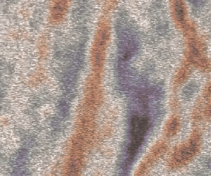
3.3. Snow particle concentration
The snow particle concentration fields provide further support to the previous arguments. Because the January 2019 dataset does not allow for locating individual particles, we characterized the concentration using the local and instantaneous image intensity  $I(x,y,t)$. This approach is based on the observation that scattered light intensity varies linearly with the particle number density $N$ for monodisperse particles (Bernard & Wallace Reference Bernard and Wallace2002) and with $N\overline {d_s}^2$ for polydisperse particles (Raffel, Willert, Scarano, Kähler & Wereley Reference Raffel, Willert, Scarano, Kähler and Wereley2018), and it is often used to measure relative concentration in particle-laden flows (e.g. Lai et al. Reference Lai, Chan, Law and Adams2016). We thus calculate the relative concentration as $C^* = I/\bar {I}_{1\mathrm {min}}$, where $\bar {I}_{1\mathrm {min}}$ is the 1 min moving average of the image intensity at each location. This normalization helps attenuate temporal fluctuations of the lighting conditions (e.g. due to the power fluctuation of the searchlight) and does not affect the observed trends. We also note that using particle counting for January 2016 and November 2018 leads to the same conclusions for those datasets.
Figure 9(a) presents the p.d.f. of  $C^*$ for the three datasets, indicating different levels of spatio-temporal variability. January 2016 displays an approximately Gaussian distribution (with a kurtosis of 3.5, closely matched to the kurtosis of 3 from a Gaussian distribution), while January 2019 exhibits stretched exponential tails (kurtosis of 4.9), pointing to the significant likelihood of exceptionally low-/high-concentration events. The trend across the cases parallels that of $Re_\lambda$: the more intense the turbulence, the higher the variance and intermittency in the concentration fields. Figure 9(b) illustrates a sample $C^*$ field from January 2019, for which the standard deviation of the concentration exceeds 10 % of the mean. This representative snapshot clearly shows relatively dense zones, vertically elongated and interleaved with more dilute ones. We characterize such spatial clustering in the next section. Here we stress that the more turbulent cases display stronger clustering, and that the latter is typically concurrent with settling enhancement by preferential sweeping (Aliseda et al. Reference Aliseda, Cartellier, Hainaux and Lasheras2002; Baker et al. Reference Baker, Frankel, Mani and Coletti2017; Petersen et al. Reference Petersen, Baker and Coletti2019; Momenifar & Bragg Reference Momenifar and Bragg2020).

Figure 9. (a) The p.d.f. of snow particle relative concentration  $C^*$. Black solid, dotted and dashed lines correspond to the January 2016 ( $Re_\lambda = 938$), November 2018 ( $Re_\lambda = 3545$) and January 2019 ( $Re_\lambda = 9180$) data, respectively. (b) Instantaneous $C^*$ field from January 2019.
Direct evidence of preferential sweeping in the more turbulent datasets is provided by the correlation between the local concentration and the simultaneous vertical velocity. In figure 10 we plot the PIV-based vertical velocity of the snow particles conditioned by the local concentration. Because the latter is available at every pixel, we use its spatial average in each PIV interrogation window. The level of correlation between concentration and fall speed is marginal for January 2016, significant for November 2018 and the strongest for January 2019. Analogous trends were reported since the first demonstration of preferential sweeping by Wang & Maxey (Reference Wang and Maxey1993), and recently confirmed in various simulations and laboratory experiments (among others, Aliseda et al. (Reference Aliseda, Cartellier, Hainaux and Lasheras2002), Baker et al. (Reference Baker, Frankel, Mani and Coletti2017), Huck et al. (Reference Huck, Bateson, Volk, Cartellier, Bourgoin and Aliseda2018) and Petersen et al. (Reference Petersen, Baker and Coletti2019)). This is a strong indication that the relatively large settling velocity of November 2018 and January 2019 (compared to diameter-based expectations) is due to the snow particles preferentially sampling downward air flow regions.

Figure 10. Ensemble-averaged snow particle settling velocity conditioned on value of the local relative concentration  $C^*$ and normalized by the unconditional mean settling velocity. Symbols as in figure 7.
3.4. Snow particle clustering
In the above we have shown evidence that suggests how snow particles respond to air velocity fluctuations similarly to small inertial particles in turbulence. It is then of interest to characterize the appearance of one of the most striking effects of particle–turbulence interaction: spatial clustering. In the following we describe the properties of clusters identified using approaches analogous to those in previous laboratory studies. While quantitative comparisons are thwarted by the uncertainty on the snow particles Stokes number, we show that the concentration fields display the hallmark features repeatedly reported in laboratory studies.
We focus specifically on the January 2019 case, which presents the most intense turbulence and the most inhomogeneous concentration. We follow Aliseda et al. (Reference Aliseda, Cartellier, Hainaux and Lasheras2002) and identify clusters as connected regions where the concentration  $C^*$ is above a prescribed threshold. This approach is standard in image object segmentation, and it has been applied to passive scalars, enstrophy and velocity fluctuations to detect coherent flow structures in turbulence (Catrakis & Dimotakis Reference Catrakis and Dimotakis1996; Moisy & Jiménez Reference Moisy and Jiménez2004; Lozano-Durán, Flores & Jiménez Reference Lozano-Durán, Flores and Jiménez2012; Carter & Coletti Reference Carter and Coletti2018). In order to select an objective threshold $C_{thold}^*$, we analyse the percolation behaviour of the identified objects (Moisy & Jiménez Reference Moisy and Jiménez2004). For higher values of the threshold only a few small clusters are detected, which grow in size and number up to a maximum as the threshold is lowered. They then start to merge, their number decreasing until a single macro-cluster occupies the entire domain. This process is illustrated in figure 11, highlighting the chosen threshold which corresponds to the maximum number of identified clusters (Lozano-Durán et al. Reference Lozano-Durán, Flores and Jiménez2012; Carter & Coletti Reference Carter and Coletti2018). We disregard those that touch the image border, as their full spatial extent could be underestimated. The planar nature of the measurement limits our ability to fully characterize the cluster geometry. However, comparison between previous planar measurements characterizing coherent turbulence structures (Carter & Coletti Reference Carter and Coletti2018) and inertial particle clusters (Petersen et al. Reference Petersen, Baker and Coletti2019) indicates that two-dimensional imaging successfully and quantitatively captures the important features identified in full three-dimensional datasets.

Figure 11. Average number of clusters per image as a function of relative concentration threshold  $C^*_{thold}$. The inset shows clusters in a binarized concentration field (corresponding to the field shown in figure 9b) using the threshold that maximizes the number of detected clusters (vertical dashed line in the plot).
Similar to previous imaging studies of particle-laden turbulence, we consider the p.d.f. of the cluster area  $A_c$ normalized by the Kolmogorov scale (figure 12a). The slope displays a marked change above a length scale corresponding to the light sheet thickness (below which the likelihood of imaging overlapping objects prevents their characterization). Larger clusters show a power-law decay of the area distribution over more than a decade. This suggests self-similarity between clusters of different sizes, pointing to their origin from turbulent eddies (which are also self-similar (Moisy & Jiménez Reference Moisy and Jiménez2004; Baker et al. Reference Baker, Frankel, Mani and Coletti2017)). The power-law exponent is consistent with the previously reported value of $-2$ (Monchaux, Bourgoin & Cartellier Reference Monchaux, Bourgoin and Cartellier2010; Petersen et al. Reference Petersen, Baker and Coletti2019), while applying the same method to a random intensity field would yield a much narrower distribution (Sanada Reference Sanada1991). The detected objects can reach linear dimensions of several metres. While this challenges the classic estimates of inertial particle clusters being ${O}(10\eta )$ in size (Eaton & Fessler Reference Eaton and Fessler1994), there is mounting experimental evidence, from Voronoi tessellation analysis, that the cluster size increases with the flow Reynolds number (Sumbekova et al. Reference Sumbekova, Cartellier, Aliseda and Bourgoin2017). Moreover, whereas radial distribution functions (RDFs) calculated from three-dimensional simulations display high levels mostly for separations below ${O}(10\eta )$, this is influenced by the fact that the clusters are typically much thinner in one dimension than in the other two (Baker et al. Reference Baker, Frankel, Mani and Coletti2017).

Figure 12. (a) The p.d.f. of snow particle cluster area normalized by Kolmogorov scaling, showing a power-law decay with an exponent close to  $-2$ for sizes larger than the light sheet thickness (vertical dashed line). (b) Scatter plot of cluster perimeter versus square root of the cluster area, both normalized by Kolmogorov scaling.
To further describe the cluster topology, figure 12(b) shows a scatter plot of their perimeters versus the square root of their areas. For small clusters, the data points follow a power law with unit exponent, as expected for regular two-dimensional objects. Such a trend is inherently impacted by the light sheet thickness. For larger ones (especially for sizes far larger than the light sheet thickness) the exponent is significantly higher, indicating a convoluted structure of the cluster borders. This trend was observed in several previous imaging studies of particle-laden turbulence (Aliseda et al. Reference Aliseda, Cartellier, Hainaux and Lasheras2002; Monchaux et al. Reference Monchaux, Bourgoin and Cartellier2010; Petersen et al. Reference Petersen, Baker and Coletti2019) and is consistent with the view of inertial particle clusters as fractal sets (Calzavarini et al. Reference Calzavarini, Kerscher, Lohse and Toschi2008).
Clusters of heavy particles settling in turbulence are known to be elongated and preferentially aligned with the vertical direction (Woittiez, Jonker & Portela Reference Woittiez, Jonker and Portela2009; Dejoan & Monchaux Reference Dejoan and Monchaux2013; Ireland et al. Reference Ireland, Bragg and Collins2016b; Baker et al. Reference Baker, Frankel, Mani and Coletti2017; Petersen et al. Reference Petersen, Baker and Coletti2019). Figure 13(a) reports the p.d.f. of the cluster aspect ratio (obtained by ellipse-fitting as for the snow particle images from DIH). The peak slightly below 0.5 is consistent with the laboratory study of Petersen et al. (Reference Petersen, Baker and Coletti2019), who found the distribution to be robust for a range of physical parameters. The p.d.f. of the angle  $\theta _c$ made by the ellipse major axis with the horizontal (figure 13b) confirms a strong prevalence of vertically oriented clusters. The weak prevalence of less than $90^{\circ }$ clusters is likely the consequence of the significant wind speed and mean shear.

Figure 13. The p.d.f.s of (a) aspect ratio and (b) orientation angle of snow particle clusters.
Finally, we consider the cluster fall speed  $W_c$, obtained by averaging the vertical velocity at all locations belonging to a given cluster. This is then ensemble-averaged over all clusters of a certain size, normalized by the mean settling velocity $W_s$ and plotted against the cluster area (figure 14). Overall, clusters fall significantly faster than $W_s$, in keeping with the velocity–concentration correlation shown above. Also, there is an apparent trend of increasing fall speed with cluster size, as seen in laboratory experiments (Huck et al. Reference Huck, Bateson, Volk, Cartellier, Bourgoin and Aliseda2018; Petersen et al. Reference Petersen, Baker and Coletti2019). While this could be merely due to the preferential sampling of downward flow regions, the sharp increase of $W_c$ above a certain cluster size suggests that a more complex interaction between the snow and the turbulent air may be taking place.

Figure 14. Normalized cluster velocity as a function of cluster size.
The estimated particle volume fraction for January 2019 is above  $10^{-6}$ (table 3) and it may approach $10^{-5}$ in the denser clusters. According to widespread criteria for gas–solid flows (Elghobashi Reference Elghobashi1994; Balachandar & Eaton Reference Balachandar and Eaton2010), in this range of concentrations the dispersed phase is expected to exert a significant back-reaction on the carrier fluid (so-called two-way coupling). Therefore, the larger clusters, by virtue of the simultaneous action of large numbers of particles, may be able to collectively drag air down with them, enhancing their fall speed beyond that granted by one-way coupling mechanisms like preferential sweeping. Such an effect has been proposed to explain settling velocities observed at similar volume fractions in experiments (Aliseda et al. Reference Aliseda, Cartellier, Hainaux and Lasheras2002; Huck et al. Reference Huck, Bateson, Volk, Cartellier, Bourgoin and Aliseda2018) and numerical simulations (Bosse, Kleiser & Meiburg Reference Bosse, Kleiser and Meiburg2006; Frankel et al. Reference Frankel, Pouransari, Coletti and Mani2016). In fact, the S-shape of the velocity versus concentration curve in figure 10 resembles the recent results of Huck et al. (Reference Huck, Bateson, Volk, Cartellier, Bourgoin and Aliseda2018), who explained their findings using collective particle effects.
4. Conclusions
The present results provide evidence that atmospheric turbulence affects not only the variance, but also the mean of the snow settling velocity. Specifically, we show that seemingly contradictory trends between snow particle diameters and fall speeds can be explained by the ability of turbulence to enhance settling. This effect is attributed to the preferential sweeping of particles into downward regions of the air flow, which is known to be most intense for particles with Stokes number  $St = {O}(1)$ based on Kolmogorov scaling. The effect depends therefore on the coupling between the hydrometeor properties and the atmospheric turbulence. This explanation is consistent with the observed acceleration distributions, from which we infer the range of $St$ for different datasets. We record large acceleration variance for the case with a fall speed substantially larger than the air velocity fluctuations. We deduce that, for these snow particles, the crossing trajectory effect (caused by gravitational drift) dominates over the preferential sampling effect (due to the particle inertia): these hydrometeors quickly drift away from the local turbulent structures and are not strongly clustered by them. On the other hand, preferential sweeping is strong when turbulence fluctuations are comparable to gravitational drift. The clearest demonstration of preferential sweeping is found in the vertical velocity conditioned by the local concentration: regions of high concentration display higher settling velocities. This might also imply a back-reaction of the particles on the flow through collective drag. Our estimates of the highest volume fractions are indeed above classic thresholds for two-way coupling, although one should use caution in applying those to a flow laden with complex particles. We have also demonstrated that, in the cases where strong preferential sweeping is inferred, the concentration field is highly non-uniform. Clusters appear over a wide range of scales, displaying signature features identified in laboratory experiments and numerical simulations: power-law size distribution, fractal-like silhouette, vertical elongation and large fall speed that increases with size.
Taken together, these results confirm and extend the conclusion of Nemes et al. (Reference Nemes, Dasari, Hong, Guala and Coletti2017): the phenomenology of inertial particles in turbulence, built over decades of canonical flow studies, is largely applicable to the dynamics of snow settling in air. Presently, none of these well-known concepts are incorporated in weather forecasting models. Other recent studies, also imaging-based, demonstrated that those concepts are in fact directly applicable to atmospheric flows: within clouds, clustering of droplets was recently observed using airborne holographic instruments (Beals et al. Reference Beals, Fugal, Shaw, Lu, Spuler and Stith2015; Larsen et al. Reference Larsen, Shaw, Kostinski and Glienke2018), and elongated regions devoid of droplets were identified at a mountain-top station (Karpińska et al. Reference Karpińska2019).
Environmental flows give access to much larger ranges of scales than laboratory or numerical experiments, enabling the exploration of fundamental fluid mechanics questions. To our knowledge, the present field work represents the highest Reynolds number flow measurements in which inertial particle clustering is observed and quantified. The fact that we observe very large clusters (up to the integral scales of the turbulence) lends support to recent claims that these clusters grow larger with  $Re_\lambda$ (Sumbekova et al. Reference Sumbekova, Cartellier, Aliseda and Bourgoin2017), and that increasing $Re_\lambda$ extends the range of scales to which the particles respond (Tom & Bragg Reference Tom and Bragg2019). Of course, the non-canonical aspects of naturally occurring particle-laden flows have to be considered. In particular, the morphology of snow particles is expected to play an important role, especially for complex-shaped and elongated snow particles (Westbrook & Sephton Reference Westbrook and Sephton2017). Our understanding of the interaction of anisotropic particles with turbulence has seen tremendous progress in recent years (Voth & Soldati Reference Voth and Soldati2017), and imaging studies capable of testing these dynamics in the field are warranted. This will require three-dimensional imaging at high spatial and temporal resolution, and will benefit from novel capabilities now available for Lagrangian tracking (see e.g. Guala et al. (Reference Guala, Liberzon, Hoyer, Tsinober and Kinzelbach2008a) and the recent review by Discetti & Coletti (Reference Discetti and Coletti2018)).
An important aspect that the present study cannot directly address is represented by the hydrometeor collision rate, and the impact that turbulence has on it. This is expected to be strongly related to the polydispersity of the snow particles. Polydispersity drives the classic (gravitational) mechanism by which larger particles fall faster than and collide with smaller ones (Pruppacher & Klett Reference Pruppacher and Klett1997). Recent simulations, however, show that turbulence enhances the relative velocity of polydisperse particles also in the horizontal direction (Dhariwal & Bragg Reference Dhariwal and Bragg2018). Fundamental studies in this area are needed to extend the applicability of particle–turbulence dynamics to environmental flows. Additionally, field studies are warranted to investigate the correlation between the level of collision-driven aggregation and atmospheric turbulence.
Acknowledgements
The authors thank engineers from St Anthony Falls Laboratory, including J. Tucker, J. Mullin, C. Ellis, J. Marr, C. Milliren and D. Christopher, for their assistance in the experiments.
Funding
The authors gratefully acknowledge the support of the US National Science Foundation through grant NSF-AGS-1822192.
Declaration of interests
The authors report no conflict of interest.


 Open access