


1. Introduction
Our ability to model and control turbulent flows relies on the understanding of the interactions between structures of different characteristic length and time scales that coexist in wall-bounded turbulence (Marusic, Mathis & Hutchins Reference Marusic, Mathis and Hutchins2010a; Jiménez Reference Jiménez2018). Near-wall streaks and quasi-streamwise vortices are the smallest coherent features of a turbulent flow in the vicinity of a wall (Kline et al. Reference Kline, Reynolds, Schraub and Runstadler1967; Jeong et al. Reference Jeong, Hussain, Schoppa and Kim1997). They form the near-wall spectral peak in the premultiplied energy spectrogram of velocity fluctuations, and obey viscous scaling – meant as scaling with the friction velocity  $u_\tau ^*$ and length scale $\nu ^* / u_\tau ^*$, where $\nu ^*$ is the kinematic viscosity. In this article, an asterisk superscript $({\cdot })^*$ denotes dimensional values, whereas $({\cdot })^+$ implies that viscous scaling is used. At the other extreme, the size of the largest turbulent features scales with some characteristic length $h^*$ stemming from the geometry of the flow, such as the thickness of a turbulent boundary layer (Hutchins & Marusic Reference Hutchins and Marusic2007a) or the half-height of a channel flow (Monty et al. Reference Monty, Stewart, Williams and Chong2007); the latter convention is adopted in this paper. The most evident statistical footprint of these outer-scaling structures is the appearance of a broad large-scale spectral peak in the premultiplied energy spectrogram of streamwise and spanwise velocity fluctuations (Kim & Adrian Reference Kim and Adrian1999; Hutchins & Marusic Reference Hutchins and Marusic2007a; Lee & Moser Reference Lee and Moser2018), the magnitude of which increases with the friction Reynolds number $Re_\tau = h^* u_\tau ^* / \nu ^* = h^+$. Different taxonomies of the eddies contributing to such a peak have been proposed (Bailey & Smits Reference Bailey and Smits2010; Smits, McKeon & Marusic Reference Smits, McKeon and Marusic2011; Marusic & Monty Reference Marusic and Monty2019), which might as well be coincident; regardless, the generic term large-scale motions, or simply large scales, will be used in the following to simplify the discussion.
In recent decades, the availability of high-fidelity turbulent data at high Reynolds number has made it possible to investigate the role of large-scale motions and their interaction with small-scale near-wall turbulence (see, for instance, Cimarelli et al. Reference Cimarelli, De Angelis, Jiménez and Casciola2016; Cho, Hwang & Choi Reference Cho, Hwang and Choi2018; Kawata & Alfredsson Reference Kawata and Alfredsson2019; Lee & Moser Reference Lee and Moser2019; Jacobi et al. Reference Jacobi, Chung, Duvvuri and McKeon2021; Chiarini et al. Reference Chiarini, Mauriello, Gatti and Quadrio2022). One of the possible approaches for this task is to analyse different joint statistics of small- and large-scale flow features, once these have been separated through adequate filtering procedures. Within this approach, pursued also in the present paper, the coexistence and interaction between small and large scales are classified into three phenomena: the superposition of large-scale fluctuations at the wall (Abe, Kawamura & Choi Reference Abe, Kawamura and Choi2004) and the amplitude (Mathis, Hutchins & Marusic Reference Mathis, Hutchins and Marusic2009) or frequency (Ganapathisubramani et al. Reference Ganapathisubramani, Hutchins, Monty, Chung and Marusic2012; Vinuesa et al. Reference Vinuesa, Hites, Wark and Nagib2015; Baars, Hutchins & Marusic Reference Baars, Hutchins and Marusic2017; Iacobello, Ridolfi & Scarsoglio Reference Iacobello, Ridolfi and Scarsoglio2021) modulation of small-scale wall structures by the large scales.
Superposition, sometimes called footprinting, is related to the space-filling nature of large-scale motions. While large-scale motions induce the strongest streamwise fluctuations within the outer layer, their influence reaches the near-wall region, where their imprint can be found in both velocity fluctuations and wall-shear stress (Abe et al. Reference Abe, Kawamura and Choi2004; Hoyas & Jiménez Reference Hoyas and Jiménez2006; Schlatter et al. Reference Schlatter, Örlü, Li, Brethouwer, Fransson, Johansson, Alfredsson and Henningson2009). This is responsible for the well-documented failure of viscous scaling for the wall-parallel fluctuation intensities in the near-wall region (Örlü & Alfredsson Reference Örlü and Alfredsson2012; Eitel-Amor, Örlü & Schlatter Reference Eitel-Amor, Örlü and Schlatter2014; Monkewitz & Nagib Reference Monkewitz and Nagib2015).
Amplitude and frequency modulation (see, for instance, Baars et al. Reference Baars, Hutchins and Marusic2017) refer to the fact that the instantaneous amplitude and frequency of a small-scale signal – such as a filtered temporal velocity fluctuation signal measured by a hot-wire anemometer in the near-wall region of a turbulent boundary layer – appear to be proportional to the large-scale signal at the same position, with the small-scale amplitude and frequency leading the large-scale signal. Some authors report amplitude modulation to be asymmetric with respect to positive and negative large-scale events (Ganapathisubramani et al. Reference Ganapathisubramani, Hutchins, Monty, Chung and Marusic2012; Agostini & Leschziner Reference Agostini and Leschziner2019b). Frequency modulation has not been featured extensively in the literature, and this study will focus on its amplitude counterpart. Historically, amplitude modulation has been investigated by computing the single-point correlation between the large-scale streamwise velocity signal and the envelope of the small-scale one (Mathis et al. Reference Mathis, Hutchins and Marusic2009), where the latter can also be replaced by a suitable approximation (Eitel-Amor et al. Reference Eitel-Amor, Örlü and Schlatter2014), typically the small-scale velocity signal squared. Such a correlation shows positive values in the near-wall region, indicating the presence of amplitude modulation, whereas in the logarithmic layer, a so-called phase reversal is commonly observed. There, the correlation is negative, indicating that the amplitude (and frequency) of the small scales is inversely proportional to the large-scale signal, with large scales seemingly having a phase lead (Baars et al. Reference Baars, Hutchins and Marusic2017).
These single-point correlations are intimately linked to the skewness of the probability density function (p.d.f.) of the streamwise velocity (Mathis et al. Reference Mathis, Marusic, Hutchins and Sreenivasan2011b; Duvvuri & McKeon Reference Duvvuri and McKeon2015), and concerns have been raised with regard to their reliability to detect modulation (Schlatter & Örlü Reference Schlatter and Örlü2010). In this respect, Bernardini & Pirozzoli (Reference Bernardini and Pirozzoli2011) showed that using two-point correlations (or covariances) can provide a refined measure of the phenomenon. By doing so, it is revealed that the amplitude of near-wall small scales correlates well not only with the local, near-wall large-scale signal, but also with the large scales in the logarithmic layer (and more generally with the large-scale signal at almost any wall-normal position; see Agostini, Leschziner & Gaitonde Reference Agostini, Leschziner and Gaitonde2016). In contrast to the single-point correlation, the value of this inner–outer correlation is not affected by the skewness of the velocity distribution, hence it represents a credible measure.
It is also important to acknowledge that the process of quantifying modulation is in many aspects arbitrary, and yet yields robust results. Indeed, the scale decomposition of the velocity signal is inherently arbitrary in the choice of the threshold between large and small scales; moreover, different types of filters can be deployed to achieve such a decomposition. For instance, one could opt for sharp Fourier filtering as in this paper, or for a filter based on the empirical mode decomposition (Agostini & Leschziner Reference Agostini and Leschziner2019a) or on a wavelet transform (Baars et al. Reference Baars, Hutchins and Marusic2017); filtering can then be performed in time or in the streamwise direction (Mathis et al. Reference Mathis, Hutchins and Marusic2009; Baars et al. Reference Baars, Hutchins and Marusic2017), or in the spanwise direction (Bernardini & Pirozzoli Reference Bernardini and Pirozzoli2011). Finally, many different correlation or covariance coefficients have been defined in the literature for the measurement of modulation (Dogan et al. Reference Dogan, Örlü, Gatti, Vinuesa and Schlatter2019), all of which constitute a valid choice. Independently of the chosen approach, the picture of modulation phenomena that one obtains matches the one described above, as has been shown by Dogan et al. (Reference Dogan, Örlü, Gatti, Vinuesa and Schlatter2019).
Although initial studies on the matter understood and modelled modulation as an inner–outer mechanism (Hutchins & Marusic Reference Hutchins and Marusic2007b; Mathis et al. Reference Mathis, Hutchins and Marusic2009; Marusic, Mathis & Hutchins Reference Marusic, Mathis and Hutchins2010b; Mathis, Hutchins & Marusic Reference Mathis, Hutchins and Marusic2011a), the idea that prevailed later is that small scales near the wall are modulated by near-wall, superimposed large ones (Baars et al. Reference Baars, Hutchins and Marusic2017). These two ideas are not necessarily contradicting, and indeed the latter idea was already present in the former studies; the wall-normal coherence of the large scales implies that the near-wall large-scale signal can be a reasonable estimate of the outer-layer one, and vice versa (Mathis et al. Reference Mathis, Hutchins and Marusic2009; Bailey & Smits Reference Bailey and Smits2010). Jiménez (Reference Jiménez2012) showed that profiles of the streamwise fluctuation intensity associated with regions of enhanced or diminished large scales collapse when scaled with the local friction velocity; moreover, there is a correlation between the sign of the large-scale velocity gradient and the fluctuation intensities all across the channel. Modulation has been interpreted as the response of small scales to large-scale fluctuations of the wall-shear stress caused by superposition (Ganapathisubramani et al. Reference Ganapathisubramani, Hutchins, Monty, Chung and Marusic2012; Mathis et al. Reference Mathis, Marusic, Chernyshenko and Hutchins2013; Hutchins Reference Hutchins2014); this was later formalised by the quasi-steady quasi-homogeneous theory of Zhang & Chernyshenko (Reference Zhang and Chernyshenko2016). Agostini & Leschziner (Reference Agostini and Leschziner2019a) elaborated further on this, linking modulation to a local increase of the production of small scales caused by the large-scale shear stress. Involvement of the large-scale shear instead of the velocity in modulation mechanisms can also explain why one of the walls of a Couette flow exhibits an atypical negative modulation region (Pirozzoli, Bernardini & Orlandi Reference Pirozzoli, Bernardini and Orlandi2011).
Amplitude modulation has also been linked to the spanwise converging and diverging motions induced at the wall by large-scale log-layer circulations. Toh & Itano (Reference Toh and Itano2005) observed from instantaneous flow snapshots that near-wall low-speed streaks seem to cluster and merge below log-layer low-speed structures. They thus conjectured the presence of a co-supporting cycle, in which large-scale sweeps (high-speed regions associated with a downward fluctuation) at the wall energise near-wall small scales, favouring the formation of streaks. These streaks then drift under the influence of large-scale spanwise motions, so that they cluster below log-layer low-speed regions; the streaks would then merge and burst, feeding a large-scale ejection (a low-speed region associated with an upward motion) and thus the large-scale circulation. Later studies are in substantial agreement concerning the presence of wall-penetrating circulatory motions associated with log-layer sweeps and ejections (Hutchins & Marusic Reference Hutchins and Marusic2007b; Hwang et al. Reference Hwang, Lee, Sung and Zaki2016; Hwang & Sung Reference Hwang and Sung2017); the associated spanwise motions are also likely to advect near-wall streaks (Zhou, Xu & Jiménez Reference Zhou, Xu and Jiménez2022). The modulation of near-wall spanwise fluctuations by large-scale sweeps has been observed (Agostini & Leschziner Reference Agostini and Leschziner2014; Hwang et al. Reference Hwang, Lee, Sung and Zaki2016); also, log-layer sweeps and ejections have been linked to increased and decreased values of the near-wall swirling strength (Hutchins & Marusic Reference Hutchins and Marusic2007b; Hwang & Sung Reference Hwang and Sung2017) and of the local skin friction (Hwang & Sung Reference Hwang and Sung2017). However, the idea of near-wall streaks clustering below log-layer low-speed regions as proposed by Toh & Itano (Reference Toh and Itano2005) contrasts with the notion of frequency modulation, as one would expect the streak spacing to increase in correspondence of negative large-scale events (see also Zhou et al. Reference Zhou, Xu and Jiménez2022); moreover, quantitative evidence regarding the bottom-up effect described by Toh & Itano (Reference Toh and Itano2005) is contradictory (Hwang et al. Reference Hwang, Lee, Sung and Zaki2016; Zhou et al. Reference Zhou, Xu and Jiménez2022).
The common theme of all these theories and models is that modulation phenomena are tied intimately to the presence of large-scale motions at the wall, be it in the form of a large-scale gradient or of a wall-penetrating circulatory motion; it is this idea that we want to challenge with the present work. Assessing the causal relationship between superposition and modulation is challenging under natural circumstances, since these phenomena occur simultaneously; we hence devise a numerical strategy to artificially remove either of the two, so to verify whether the other phenomenon persists when isolated. Details of the numerical dataset generated for this study are provided in § 2, alongside a discussion of how amplitude modulation is measured and general details of the forcing used to suppress the two phenomena. A case-specific formulation of the forcing is discussed in § 2.1 for the suppression of superposition, and in § 2.2 for the suppression of modulation; results are presented in § 3. Finally, § 4 contains a summarising remark.
2. Numerical experiments
In the following, the streamwise, wall-normal and spanwise axes of a fully-developed turbulent channel flow are denoted by  $x$,
$x$,  $y$ and $z$, respectively; the corresponding velocity components are $u$,
$u$,  $v$ and $w$. When no superscript is provided, lengths are made non-dimensional with the channel half-height $h^*$; velocities are always reported in wall units, although the $({\cdot })^+$ superscript is sometimes dropped in the discussion when the scaling is not relevant. Let $\left \langle {{\cdot }} \right \rangle$ denote averaging along directions of statistical homogeneity and time; the fluctuation of a generic velocity component, for instance the streamwise one $u'$, is given by the Reynolds decomposition of the velocity itself, $u' = u - \left \langle {u} \right \rangle$.
The analysis of the present work relies on a newly produced direct numerical simulations (DNS) database of turbulent channel flows at friction Reynolds number  $Re_\tau = 1000$ in streamwise and spanwise periodic domains; its peculiarity is the selective suppression of either modulation or superposition phenomena, which is discussed below. The simulations are performed with the mixed-discretisation spectral solver for the incompressible Navier–Stokes equations in divergence-free wall-normal velocity and vorticity formulation by Luchini & Quadrio (Reference Luchini and Quadrio2006) at constant pressure gradient. As for the size of the computational domain, we resort to both moderately long streamwise domains (LSDs), in which the streamwise periodicity is $L_x^*/h^* = 4{\rm \pi}$, and minimal streamwise units (MSUs), for which $L_x^*/h^* = 0.4 h$ (Abe, Antonia & Toh Reference Abe, Antonia and Toh2018). MSUs are used here by virtue of their simplified flow physics and reduced computational cost; their suitability for the study of amplitude modulation is also assessed. All other discretisation parameters are set to values that are standard in DNS practice; a summary can be found in table 1.
Table 1. Details of the long streamwise domain (LSD) and minimal streamwise unit (MSU) simulations, where  $L_x^*$ and $L_z^*$ are the streamwise and spanwise extents of the computational box, and $N_x$ and $N_z$ are the numbers of Fourier modes in the homogeneous directions (additional modes are used for dealiasing, according to the $3/2$ rule), while $N_y$ is the number of collocation points in the wall-normal direction. The resulting spatial resolutions $\Delta x^+$ and $\Delta z^+$ in the streamwise and spanwise directions, respectively, as well as the wall-normal resolution $\Delta y^+_{{min}}$ at the wall, are reported. Here, $T^*$ is the temporal interval over which statistics have been collected after discarding the transient.

To quantify amplitude modulation (AM), we resort to the two-point scale-decomposed skewness  $C_{{AM}}^\ast$ (Schlatter & Örlü Reference Schlatter and Örlü2010; Bernardini & Pirozzoli Reference Bernardini and Pirozzoli2011; Mathis et al. Reference Mathis, Marusic, Hutchins and Sreenivasan2011b; Eitel-Amor et al. Reference Eitel-Amor, Örlü and Schlatter2014):
 \begin{equation} C_{{AM}}^\ast= \left\langle { {u_{SS}^+}^2 (y_{SS}^+) \, u_{LS}^+(y_{LS}^+) } \right\rangle , \end{equation}
where  $u_{LS}$ and $u_{SS}$ indicate, respectively, the low- and high-pass filtered streamwise velocity fluctuation signals, at two different wall-normal positions $y_{LS},y_{SS}$. Notice that the asterisk in $C_{{AM}}^\ast$ is kept for consistency with the literature and does not indicate that $C_{{AM}}^\ast$ is a dimensional quantity. Positive values of $C_{{AM}}^\ast$ indicate the presence of amplitude modulation, whereas negative values indicate a region of phase reversal. This $C_{{AM}}^\ast$ has been preferred to many other statistics available in the literature (see, for instance, Dogan et al. Reference Dogan, Örlü, Gatti, Vinuesa and Schlatter2019) owing to the fact that it is not normalised by ${\left \langle {u_{LS} ^+u_{LS} ^+} \right \rangle }\phantom {.}^{1/2}$. Indeed, as will be explained below in the context of suppression of superposition, the large-scale signal $u_{LS} ^+$ is damped in specific portions of the channel, thus yielding $\left \langle {u_{LS} ^+u_{LS} ^+} \right \rangle \to 0$. Filtering is performed in the spanwise direction with a sharp Fourier filter; a conventional threshold wavelength $\lambda _{z,c}^+ = h^+ / 2 = 500$ is used (see, for instance, Bernardini & Pirozzoli (Reference Bernardini and Pirozzoli2011), at a similar value of $Re_\tau$), unless stated explicitly. In the context of suppression of modulation, practical considerations led to a choice $\lambda _{z,c}^+ = h^+ = 1000$.
The suppression of either superposition or modulation is achieved by artificial damping of selected turbulent motions via a volume-force term  ${\boldsymbol {f}}$ added to the right-hand side of the momentum balance of the incompressible Navier–Stokes equations, such that
 $$\begin{gather} \frac{\partial\boldsymbol{u}^+}{\partial t} + \left(\boldsymbol{u}^+ \boldsymbol{\cdot}\boldsymbol{\nabla}\right)\boldsymbol{u}^+ =- {\boldsymbol{\nabla}} p^++ \frac{1}{Re_\tau}\,\nabla^2 \boldsymbol{u}^+ + \boldsymbol{f} , \end{gather}$$
 $$\begin{gather}\boldsymbol{\nabla}\boldsymbol{\cdot} \boldsymbol{u}^+ = 0 , \end{gather}$$
where  $\boldsymbol {u} = ( u,v,w )$, and $p$ is the pressure. Again, notice that lengths are scaled in outer units in the equation above, so that time is made non-dimensional with $h^*/u_\tau ^*$. The artificial damping is most conveniently defined in the spectral Fourier space:
 \begin{equation} \hat{\smash{\skew1\hat{\boldsymbol{f}}}\vphantom{\hat{\small i}}} =- \frac{\alpha( \kappa_x, \kappa_z, y )}{c}\, \hat{\smash{\skew1\hat{\boldsymbol{u}}}\vphantom{\hat{\tiny 1}}}^+ , \end{equation}
where  $\hat{\smash{\skew1\hat{({\cdot })}}\vphantom{\hat{\small 1}}}$ denotes the Fourier coefficient for a given streamwise and spanwise wavenumber pair $(\kappa _x, \kappa _z )$ at a specific $y$-position. The arbitrary parameter $c$ determines the strength of the damping; its value $c^* / (h^* / u_\tau ^*) = 10^{-3}$ is chosen empirically (see, for instance, Stroh et al. Reference Stroh, Hasegawa, Schlatter and Frohnapfel2016; Forooghi et al. Reference Forooghi, Stroh, Schlatter and Frohnapfel2018) to achieve a forcing that is as small as possible, while still ensuring satisfactory damping of the selected modes. The dimensionless function $\alpha ( \kappa _x, \kappa _z, y )$ selects which scales and wall-normal locations are damped, and is defined in the following, depending on whether superposition (denoted by subscript ${S}$, $\alpha _{{S}}$) or modulation ( $\alpha _{{AM}}$) is removed.
Notice that the forcing is active on all components of velocity, although the amplitude modulation analysis is carried out only on the streamwise component. Moreover, the equations of motion are solved using the wall-normal velocity and vorticity formulation that automatically fulfils the divergence-free constraint. Although the forcing that we use might have non-zero divergence (just like the nonlinear term of (2.2)), only its solenoidal component affects the governing equations – so the continuity equation (2.3) is verified at all times.
2.1. Suppression of superposition
A straightforward way of suppressing superposition of large scales at the wall is damping spanwise Fourier modes contributing to  $u_{LS}$ in that region. While this clearly defines the scales at which modal damping is activated ( $\lambda _z^+ > h^+/2$, owing to the definition of $u_{LS}$ in § 2), the wall-normal portion of the domain in which this is done is yet to be specified. To address this issue, we propose a definition of the space-scale region in which superposition takes place as the one where large near-wall motions are fed energy from other scales and wall normal positions; this region can be identified rigorously by analysing the spectral turbulent kinetic energy (TKE) budget decomposed in spanwise Fourier modes (Cho et al. Reference Cho, Hwang and Choi2018):
 \begin{equation} \frac{\partial \left\langle {\hat{e}\,} \right\rangle ^+_{x,t}}{\partial t^+} = \hat{\mathcal{P}}^++ \hat{\epsilon}^+ + \hat{\mathcal{T}}_t^++ \hat{\mathcal{T}}_p^++ \hat{\mathcal{T}}_\nu^+= 0 . \end{equation}
Here,  $\hat {({\cdot })}$ represents the coefficient of the spanwise Fourier transform associated with wavenumber $\kappa _z = 2{\rm \pi} / \lambda _z$, where $\lambda _z$ is the spanwise wavelength, and
 \begin{equation} \Bigl\langle
{\hat{e}\,} \Bigr\rangle _{x,t}^+ \left(y^+, \kappa_z^+
\right) = \tfrac{1}{2} \left.\left\langle {
|\widehat{u^\prime}|^2 + |\widehat{v^\prime}|^2 +
|\widehat{w^\prime}|^2 } \right\rangle \right._{x,t}^+
\end{equation}
\begin{equation} \Bigl\langle
{\hat{e}\,} \Bigr\rangle _{x,t}^+ \left(y^+, \kappa_z^+
\right) = \tfrac{1}{2} \left.\left\langle {
|\widehat{u^\prime}|^2 + |\widehat{v^\prime}|^2 +
|\widehat{w^\prime}|^2 } \right\rangle \right._{x,t}^+
\end{equation}
is the TKE. Averaging is performed here only in time and in the streamwise direction (hence not in the homogeneous  $z$-direction), as denoted by the subscript $\left \langle {{\cdot }} \right \rangle _{x,t}$. The terms $\hat {\mathcal {P}}$ and $\hat {\epsilon }$ denote turbulent production and dissipation, respectively, while $\hat {\mathcal {T}}_t$, $\hat {\mathcal {T}}_p$ and $\hat {\mathcal {T}}_\nu$ are turbulent, pressure and viscous transport, respectively. Particular focus lies on the turbulent transport
 \begin{equation} \mathcal{\hat{T}}_{t}^+= {\rm Re} \left. \left\langle { -\left(\widehat{u^\prime_i}^+\right)^H \frac{\partial }{\partial x_j^+} \widehat{u^\prime_i u^\prime_j}^+} \right\rangle \right._{x,t} , \end{equation}
and turbulent dissipation
 \begin{equation} \hat{\epsilon}^+ =- \left. \left\langle { \left(\frac{\partial \widehat{u^\prime_i}^+}{\partial x_j^+}\right)^H \frac{\partial \widehat{u^\prime_i}^+}{\partial x_j^+}} \right\rangle \right._{x,t} , \end{equation}
where the superscript  $({\cdot })^H$ denotes the complex conjugate, and ${\rm Re}$ indicates the real part of a complex number. As reported by Cho et al. (Reference Cho, Hwang and Choi2018) and Lee & Moser (Reference Lee and Moser2019), these two terms dominate the TKE budget in the vicinity of the wall for large wavelengths $\lambda _z$ (small $\kappa _z$); while by definition turbulent dissipation subtracts energy from given Fourier modes, turbulent transport can actually feed them power (when $\mathcal {\hat {T}}_{t}>0$), thus being suitable for the identification of superposition modes.
From our definition and figure 1, which shows  $\hat {\mathcal {T}}_{t}^+$ and $\hat {\epsilon }^+$ for the reference MSU and LSD cases, we identify the near-wall region in which superposition is suppressed as $2.3 (y^+ )^2 \leqslant \lambda _z^+$, as this region corresponds to the near-wall positive peak of $\mathcal {T}_{t}^+$; in other words, large scales are here being fed energy. A similar locus was identified by Cho et al. (Reference Cho, Hwang and Choi2018).
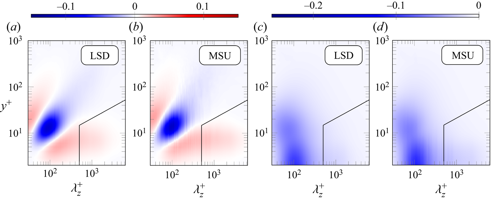
Figure 1. Premultiplied spanwise spectra of (a,b) the turbulent transport  $\kappa _z^+\mathcal {T}_{t}^+$, and (c,d) the dissipation term $\kappa _z^+\epsilon ^+$, of the spectral TKE budget. Both the reference (unperturbed) LSD and MSU cases are reported. The solid black lines mark the boundaries of the region in which modal damping is performed.
This complements the criterion  $\lambda _z^+ > h^+/2$ that defines $u_{LS}$; the complete boundaries of the space-scale region suppressed in this section are shown in figure 1. As desired, the near-wall turbulent dissipation peak (figures 1c,d), which is commonly associated with small scales, is excluded from the definition of the large, superposed ones. The following expression for $\alpha _{{S}}( \kappa _x^+, \kappa _z^+, y^+ )$ stems from the present discussion:
 \begin{equation} \alpha_{{S}}( \kappa_x^+, \kappa_z^+, y^+ ) = \begin{cases} 1, & \text{if } \kappa_z^+ \leqslant \min \left( \dfrac{2 {\rm \pi}}{500}, \dfrac{2 {\rm \pi}}{2.3 \left(y^+\right)^2} \right)\ \text{except } \kappa_x^+=\kappa_z^+=0, \\ 0, & \text{otherwise}. \end{cases} \end{equation}
Note that mode  $(\kappa _x^+, \kappa _z^+) = (0,0)$ is not damped, since this corresponds to the instantaneous streamwise and spanwise spatial average; other than that, the value of $\kappa _x$ plays no role, meaning that all $\kappa _x$ modes are suppressed if the condition on $\kappa _z$ is verified. While similar damping strategies have been attempted in the literature (see, for instance, de Giovanetti, Hwang & Choi Reference de Giovanetti, Hwang and Choi2016), the peculiarity of the present one is that large scales are removed only in the vicinity of the wall and not throughout the whole domain.
2.2. Suppression of modulation
As for amplitude modulation, its suppression is not as trivial, and its spectral representation needs to be discussed first. Let us consider a toy problem, where a large-scale spanwise sinusoid  $\cos (\kappa _l z)$ modulates a small-scale carrier wave $\cos (\kappa _{s}z)$, where $\kappa _{l}$ and $\kappa _{s}$ are the respective wavenumbers; the Fourier representation of the large-scale signal has energy content only on the $\kappa _z = \pm \kappa _{l}$ mode (or $\kappa _z = \pm \kappa _{s}$ for the small-scale one). The modulated signal will be, for example, $[1+\cos (\kappa _{l}z)] \cos (\kappa _{s}z)$. It can be proven easily, by applying the angle addition formula for trigonometric functions (Abramowitz & Stegun Reference Abramowitz and Stegun1964), that such a modulated signal has energy content exclusively on modes $\kappa _z = \pm \kappa _{s}$, corresponding to the original carrier wave, and $\kappa _z = \pm (\kappa _{s} \pm \kappa _l)$, such modes being named sidebands.
In the context of our spectral DNS, we identify the first six non-zero spanwise discrete Fourier modes  $\kappa _z = \pm (\kappa _{z,0},\ldots, 6\kappa _{z,0})$ as the large-scale, modulating signal. Bear in mind that the simulation grid is equally spaced in the Fourier- $\kappa _z$ direction, the spacing being $\kappa _{z,0} = 2 {\rm \pi}/ L_z \approx 0.898$. Consider now a generic small-scale carrier with wavenumber $\kappa _z = \kappa _s$ being modulated by the large modes; the sideband will comprise the six discrete Fourier modes preceding and following $\kappa _s$, namely $\kappa _z = \pm \kappa _s \pm (\kappa _{z,0},\ldots, 6\kappa _{z,0})$. As an example, figure 2 highlights the sideband of mode $\kappa _s = 14 \kappa _{z,0}$; the integer $n_z$ referenced there is defined as
 \begin{equation} n_z = \kappa_z^* / \kappa_{z,0}^*. \end{equation}
By suppressing the sidebands of each possible small-scale carrier in our simulation, we make amplitude modulation non-representable in our domain – in other words, we suppress it. Practically, this is done by suppressing six spanwise modes every seven for the small scales, as shown in figure 2; the effective spacing  $\Delta \kappa _z$ between non-zero (or, more precisely, non-damped) spanwise small-scale modes is thus increased from $\Delta \kappa _z = \kappa _{z,0}$ to $\Delta \kappa _z = 7\kappa _{z,0}$. This is done only in the proximity of the wall ( $y^+ \leqslant 40$), where positive modulation takes place, in order to limit intrusiveness. Hence $\alpha _{{AM}}$ is defined as
 \begin{equation} \alpha_{{AM}}( \kappa_x^+, \kappa_z^+, y^+ ) = \begin{cases} 1, & \text{if } y^+ \leqslant 40 \ \land\ n_z/7 \notin \mathbb{Z} \ \land\ n_z>6, \\ 0, & \text{otherwise}, \end{cases} \end{equation}
where  $\mathbb {Z}$ is the group of integer numbers. Once again, the value of $\kappa _x$ plays no role in the above definition, so that suppression is active for all $\kappa _x$ modes in correspondence with values of $\kappa _z$ that get suppressed.
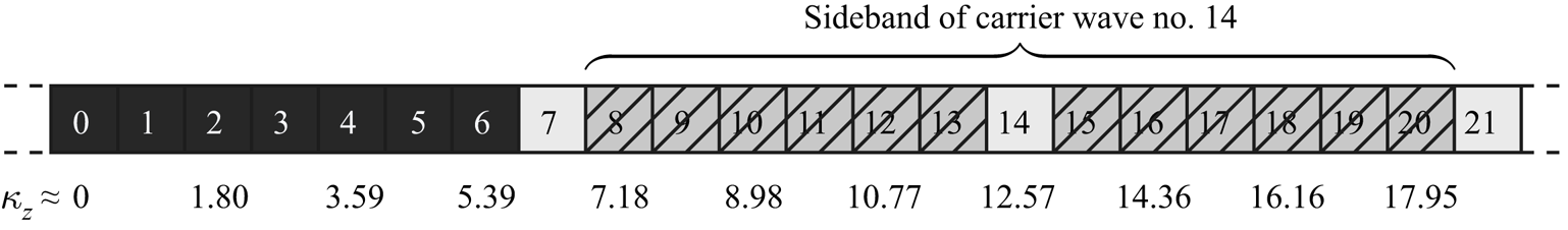
Figure 2. Schematic representation of the suppression of modulation for the discretisation used in this paper. Each box represents a spanwise Fourier mode with its value of  $n_z$; wavenumbers are reported under the boxes. Note that only low-wavenumber, positive modes are represented. Large-scale, modulating modes are coloured in black, while small-scale carrier ones are white. The modes being suppressed, namely the sideband of each carrier, are cancelled out.
Notice that the large scales are here effectively defined as having  $|n_z| < 7$, which translates to $\lambda _z^+ > h^+ = 1000$ in terms of wavelengths. This value of the large–small threshold wavelength is larger than the one stated at the beginning of this section and will be used exclusively in cases where modulation is suppressed, for instance for the calculation of $C_{{AM}}^\ast$. The different choice is meant to limit intrusiveness of the forcing: by choosing a larger threshold wavelength, not only is the bandwidth of the large scales reduced, but also the width of the sidebands of small carrier modes is reduced. Since these sidebands are being suppressed, the smaller the sidebands, the smaller the amount of energy being subtracted from the flow.
The effect of this forcing on scale interactions is better understood by considering triadic interactions (Cho et al. Reference Cho, Hwang and Choi2018) between spanwise Fourier modes. These interact in pairs through the nonlinear term of the Navier–Stokes equations, resulting in a transfer of momentum (and energy) to a third mode. Using the angle addition formula as before, it can be shown that where the forcing is active, interactions between small-scale modes cannot yield a transfer of energy to (or from) large scales, with the exception of the large  $\kappa _z = 0$ mode. Moreover, interactions between a large-scale (except $\kappa _z = 0$) mode and a smaller-scale (except $\kappa _z = 7 \kappa _{z,0}$) one would produce an energy transfer to (or from) suppressed modes; the effects of these interactions are thus nullified.
As for  $C_{{AM}}^\ast$, similar considerations show that where the forcing is active, the signal $u_{SS}^2$ has no content on large-scale Fourier modes, except for mode $\kappa _z = 0$. Thus the covariance $C_{{AM}}^\ast = \langle {u_{SS}^+}^{\text{2}} \, u_{LS} ^+ \rangle$ has at most contributions from the interaction between $u_{SS}^2$ and mode $\kappa _z = 0$ of $u_{LS}$; all other contributions are null. In other words, the only modulation-like effect that could be observed is a correlation in time (and in the streamwise direction) between the spanwise average of $u_{LS}$ and the spanwise average of $u_{SS}^2$. This is a very weak effect, as will be shown later; moreover, if it were removed, then the value of $C_{{AM}}^\ast$ should be zero, where suppression of modulation is performed.
2.3. Energy-conserving smoothed spectra
The modulation-suppressing procedure described in § 2.2 produces a banded pattern in the spanwise (co-)spectra of the Reynolds stresses, as can be seen later, in figure 13, for instance. The banded pattern not only affects the near-wall region where the forcing is active, but rather propagates to the core of the channel, making the spectra hard to visualise. We therefore define a smoothed version  $\bar {\varPhi }$ of a generic spanwise (co-)spectrum $\varPhi$ that improves readability while being energy-conserving, meaning that the correct values of the Reynolds stresses can be recovered by integrating the smoothed spectral contributions given by $\bar {\varPhi }$.
In the context of our numerical simulations, the spanwise spectrum  $\varPhi$ (at any wall-normal distance) is evaluated at a discrete set of equally spaced spanwise wavenumbers $\kappa _{z,n}=n\kappa _{z,0}$, where $n$ is a non-negative integer, yielding a set $\varPhi (\kappa _{z,n})$. The smoothed spectrum is instead evaluated at a set of spanwise wavenumbers corresponding to modes that are not suppressed, yielding a set of values $\bar {\varPhi }_j$ (where $j$ is also a non-negative integer). These are defined so that
 \begin{equation} \begin{cases} \bar{\varPhi}_j = \varPhi(\kappa_{z,\,j}), & \text{if } 0\leqslant j\leqslant6, \\ \bar{\varPhi}_j = \frac{1}{4}\sum_{i=0}^3 \varPhi(\kappa_{z,j+i}), & \text{if } j=7, \\ \bar{\varPhi}_j = \frac{1}{4}\sum_{i=-3}^0 \varPhi(\kappa_{z,n_{max}+i}), & \text{if } j=\,j_{max}, \\ \bar{\varPhi}_j = \frac{1}{7}\sum_{i=-3}^3 \varPhi(\kappa_{z,7(\,j-6)+i}), & \text{otherwise}, \end{cases} \end{equation}
where  $n_{max}$ and $j_{max}$ are the maximum values of $n$ and $j$, respectively. In other words, the spectrum is left untouched for large-scale modes; for the small-scale modes, the value of $\varPhi$ for each non-suppressed mode is averaged with the values of $\varPhi$ of the six adjacent suppressed modes (three per side) to yield a single value of $\bar {\varPhi }$. For the first ( $j=7$) and last ( $j=\,j_{max}$) small-scale modes, the average is performed on only one side, that is, with only the three preceding or successive suppressed modes. Notice that the number of points in the spanwise direction is chosen so that the mode with the highest wavenumber is not suppressed. The procedure is illustrated in figure 3, and yields a sensible spectral representation of the Reynolds stresses when applied at all wall-normal positions – including those at which the forcing is not active. See, for instance, figure 13.
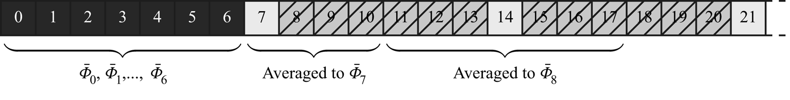
Figure 3. Schematic representation of the averaging procedure used to recover smooth (co-)spectra of the Reynolds stresses.
3. Results
To begin with, statistics of interest are reported for the reference (unperturbed) LSD and MSU cases, for reference and validation. Large-scale structures of streamwise velocity fluctuations are significantly enhanced in MSUs due to the impaired nature of the pressure–strain correlation (Abe et al. Reference Abe, Antonia and Toh2018); they are quasi-streamwise-invariant and thus lack the characteristic inclination observed in larger domains. Figure 4 shows the mean velocity profile  $U^+=\left \langle {u} \right \rangle ^+$ (figure 4a) and fluctuation intensities (figure 4b) for two LSD and MSU unperturbed simulations, used as a reference case for the numerical experiments. Both cases compare well against literature LSD data in Lee & Moser (Reference Lee and Moser2019) and MSU data in Abe et al. (Reference Abe, Antonia and Toh2018). The enhanced streamwise fluctuations of the MSU, clearly visible in figure 4(b), result in a plateau for $\left \langle {u^\prime u^\prime } \right \rangle ^+$ that is otherwise visible at much higher values of $Re$ in longer domains. On the other hand, $v^\prime$ and $w^\prime$ fluctuations have lower intensity in MSUs, and the mean velocity profile exhibits an anomalous wake region starting at $y^+ \approx 400$ (Flores & Jiménez Reference Flores and Jiménez2010). An enhancement of $u^\prime$ fluctuations in the MSU can also be observed from the spanwise one-dimensional spectrum, reported in figures 5(a,b) for the LSD and MSU cases. Although the spectra share the same qualitative behaviour, with a small-scale buffer-layer energy peak and a large-scale outer-layer one (see also Lee & Moser Reference Lee and Moser2018), both these peaks are more intense for the MSU case.
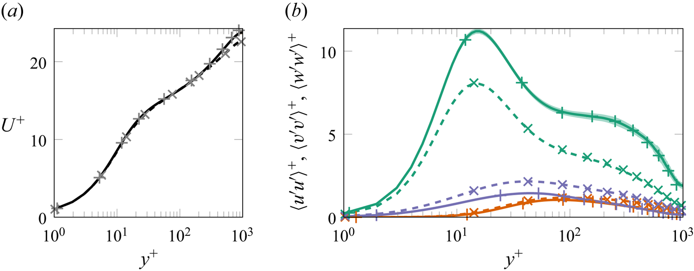
Figure 4. Profiles of (a) the mean velocity and (b) fluctuation intensities, for the unperturbed MSU (solid) and LSD (dashed) cases. Green shows  $\left \langle {u'u'} \right \rangle ^+$, red shows $\left \langle {v'v'} \right \rangle ^+$, and blue shows $\left \langle {w'w'} \right \rangle ^+$. The uncertainty at a 99.7 % confidence level quantified as described in Russo & Luchini (Reference Russo and Luchini2017) is shown for the MSU case as a shaded area. MSU data in Abe et al. (Reference Abe, Antonia and Toh2018) are marked with $+$, while $\times$ indicates LSD data in Lee & Moser (Reference Lee and Moser2015).
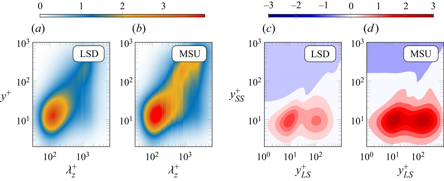
Figure 5. Reference simulations (without forcing). (a,b) Premultiplied one-dimensional spanwise spectra  $\kappa _z^+ \phi _{uu}^+$ of the streamwise velocity fluctuations. (c,d) Amplitude modulation coefficient $C_{{AM}}^\ast$; colour levels starting from zero (white) with increments of (c) ${\pm }0.3$ for LSD, and (d) ${\pm }0.5$ for MSU.
It is possibly these energised large scales, combined with the absence of their meandering, that make amplitude modulation more intense in the MSU; this can be observed from figures 5(c,d), which compare the distribution of the two-point scale-decomposed skewness  $C_{{AM}}^\ast$ for the LSD and the MSU. Apart from the intensity, the qualitative structure of the $C_{{AM}}^\ast$ map of figure 5 in the $y_{SS}^+ < 30$ region is the same for both LSD and MSU, suggesting that the smaller domain can still capture correctly scale-interaction phenomena such as amplitude modulation. In agreement with previous observations (Bernardini & Pirozzoli Reference Bernardini and Pirozzoli2011; Agostini et al. Reference Agostini, Leschziner and Gaitonde2016; Dogan et al. Reference Dogan, Örlü, Gatti, Vinuesa and Schlatter2019), two positive peaks are present at $y_{SS}^+\approx 10$, one of which lies on the diagonal of the plot ( $y_{LS}^+ \approx 10$), whereas the other will be referred to as off-diagonal ( $y_{LS}^+ \approx 150$). As discussed already, the diagonal peak of $C_{{AM}}^\ast$ is affected by the skewness of the velocity signal (Schlatter & Örlü Reference Schlatter and Örlü2010; Mathis et al. Reference Mathis, Marusic, Hutchins and Sreenivasan2011b), whereas the off-diagonal peak is not, hence constituting a more reliable detector of modulation phenomena (Bernardini & Pirozzoli Reference Bernardini and Pirozzoli2011). As expected, a negative- $C_{{AM}}^\ast$ region is also present, mainly involving small scales in the outer layer; the contour of this region becomes much more regular for the MSU case, and can be approximated by a straight horizontal line $y_{SS}^+ \approx 100$ for $y_{LS}^+ < 150$. This regularity is possibly a consequence of the lack of inclination of the large structures, which are quasi-homogeneous along the streamwise direction in the MSU cases.
A graphical representation of what the skewness coefficient  $C_{{AM}}^\ast$ quantifies is provided in figure 6. Here, the near-wall ( $y_{SS}^+ \approx 10$) small-scale activity $u_{SS}^+{}^2$ and the log-layer ( $y_{LS}^+ \approx 100$) large-scale signal $u_{LS} ^+$ from an instantaneous flow realisation of the unperturbed MSU simulation are represented in a streamwise–spanwise plane. Notice that these wall-normal coordinates correspond to the off-diagonal peak of the $C_{{AM}}^\ast$ map (figures 5c,d), and that the covariance of the two represented quantities corresponds to $C_{{AM}}^\ast$. As expected, regions of positive large scales exhibit increased values of the small-scale activity with respect to regions of negative large scales, although this correspondence is imperfect as it holds only in a statistical sense. An analogous consideration was made by Hutchins & Marusic (Reference Hutchins and Marusic2007b), who first observed amplitude modulation in experimental data, except that modulation was seen in time signals. Due to the minimal streamwise domain size, in MSUs regions of positive (or negative) large scales extend all across the streamwise domain length, whereas changes of sign of the large scales are encountered mainly along the spanwise direction. Hence in MSUs, the correlation between $u_{LS}$ and $u_{SS}^2$ is mainly to be seen in the spanwise direction.

Figure 6. Visualisation of an instantaneous streamwise velocity field on wall-parallel planes for the reference (unperturbed) MSU simulation. Colour: small-scale activity  ${u_{SS}^+}^{\text{2}}$ at $y^+ = 10$. Black lines are contours of zero large-scale fluctuations ( $u_{LS} ^+ = 0$) at $y^+ = 100$. Regions of positive large scales are shaded.
3.1. Suppression of superposition
In § 2.1, it was shown how the footprint of large scales at the wall (also known as superposition) can be removed numerically through modal damping; essentially, energy is removed from selected near-wall large scales. To validate the data produced with this forcing, some simple statistics are reported in figure 7. Figure 7(a) shows the mean velocity profile for the forced MSU and LSD cases as compared to the unperturbed simulations; as desired, the suppression strategy has no substantial effect on the mean velocity profile, either in the inner or in the wake region. The same holds for the distribution of Reynolds shear stress (figure 7b), as well as for the spanwise and wall-normal fluctuation intensities (figures 7c,d), although the forcing is active also on these two components of velocity. This suggests that the removed motions have only a marginal relevance for both the inner and outer dynamics of the flow.

Figure 7. One-point statistics for the simulations with suppression of superposition (solid line for MSU, dashed for LSD). For comparison, the same statistics are reported for the reference unperturbed cases ( $+$ for MSU, $\times$ for LSD). (a) Mean velocity profile; (b) Reynolds shear stress; (c,d) fluctuation intensities (colours as in figure 4).
The reason for the negligible effect of the forcing on the mean flow properties can be found in the spanwise co-spectra of the Reynolds shear stress, which are shown in the Appendix for simulations with and without forcing. These spectra represent the contribution of each spanwise Fourier mode to the profiles of figure 7(b). The superposition-removing forcing blocks near-wall large-scale sweeps and ejections, whose spectral contribution to  $\left \langle {u'v'} \right \rangle$ is insignificant; the $\left \langle {u'v'} \right \rangle$ profile is thus substantially unaffected by their removal, and so is the mean momentum balance in turn. This is not trivial, as the removal of near-wall large scales could also have an indirect effect on the $\left \langle {u'v'} \right \rangle$ profile owing to nonlinearities, which is not observed: the superposition appears to be linear in this context. A similar argument holds for $\left \langle {v'v'} \right \rangle$ and $\left \langle {w'w'} \right \rangle$: the space-scale region that is being suppressed contributes only marginally to the two normal stresses (spectra are not shown for brevity), hence the profiles match the ones of the unperturbed cases.
The forcing has a significant effect only on the streamwise fluctuation intensity  $\left \langle {u'u'} \right \rangle$ (figures 7c,d), which is significantly reduced in the near-wall region; this drop in TKE is expected, as the forcing subtracts power from the flow in the proximity of the wall. The drop is larger for the MSU case (figure 7c) than for the LSD case (figure 7d); indeed, as explained above, the removed large scales are more intense in the former case. As expected, towards the core of the channel, where the forcing is no longer active, profiles of $\langle {u'u'}\rangle^+$ for the perturbed cases approach the values of their unperturbed counterparts.
The effect of superposition removal is explored further by analysing the spanwise energy and turbulent transport spectrum, as well as the  $C_{{AM}}^\ast$ map. These are reported in figure 8 for the MSU case; results for the longer domain are not shown for brevity, except for the $C_{{AM}}^\ast$ map. The energy spectrum (figure 8a) and the turbulent transport one (figure 8b) indicate success of the suppressing action: not only is no energy content present for the superposition modes, as expected, but also no energy content is being deposited by $\hat {\mathcal {T}}_{t}^+$ on these modes. For wavelengths at which modal damping is active, the usual near-wall positive peak of $\hat {\mathcal {T}}_{t}^+$ vanishes, and it reappears at the nearest position to the wall where the suppressing action is absent. This also results in the negative large-scale region of $\hat {\mathcal {T}}_{t}^+$ being shifted towards the core of channel. In the outer layer, large scales still persist in spite of their suppression near the wall, as can be seen in the energy spectrum; the same was reported by Zhou et al. (Reference Zhou, Xu and Jiménez2022), who performed a similar numerical experiment. This suggests that the outer flow region has some degree of autonomy from the wall, corroborating the results of Flores & Jiménez (Reference Flores and Jiménez2006), Mizuno & Jiménez (Reference Mizuno and Jiménez2013) and Kwon & Jiménez (Reference Kwon and Jiménez2021).

Figure 8. Simulations with suppression of large-scale superposition at the wall. Premultiplied spanwise spectra of (a) the streamwise fluctuation  $\kappa _z^+\phi _{uu}^+$, and (b) the turbulent transport term $\kappa _z^+\mathcal {T}_{t}^+$, for the MSU case. Amplitude modulation coefficient $C_{{AM}}^\ast$ for the (c) LSD and (d) MSU cases. Colour map and levels as in figures 1 and 5.
Unexpected results can be observed from the  $C_{{AM}}^\ast$ maps of figures 8(c) and 8(d); while the diagonal peak predictably disappears, the off-diagonal one is not only still present, but also unaltered in intensity with respect to figure 5, indicating the persistence of modulation phenomena on small scales in the buffer layer ( $y_{SS}^+ \approx 10$). This hints at the fact that superposition and modulation are not so closely interlinked as previously thought, to the point that one phenomenon can be suppressed without significantly affecting the other. It is noteworthy, moreover, that the large-scale signal $u_{LS}$ is being entirely suppressed for $y^+ < 14.7$, whereas the small-scale signal still exhibits modulation in that region; this clearly excludes that amplitude modulation be caused entirely by the superimposed, local large scales, or by fluctuations in the wall-shear stress. Since the superposition-suppressing forcing is active on all components of velocity, there cannot be any converging or diverging spanwise large-scale motion at the wall either.
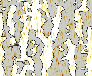
The persistence of modulation phenomena is reinforced by figure 9, showing an instantaneous realisation of the near-wall small-scale activity  $u_{SS}^+{}^2$ and of the log-layer large-scale signal $u_{LS} ^+$. No qualitative difference with respect to figure 6 can be observed, suggesting that not only does the forcing not significantly alter the flow structure, but also a correlation between the large scales and the small-scale activity is still present.
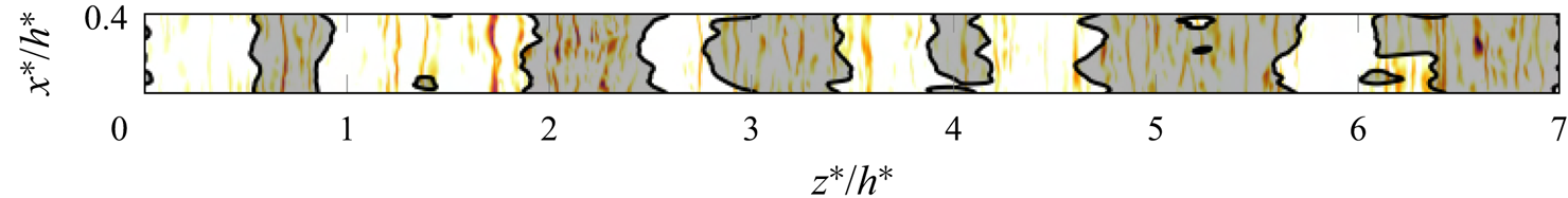
Figure 9. Visualisation of an instantaneous streamwise velocity field on wall-parallel planes for the MSU simulation with suppression of superposition. Colour indicates small-scale activity  ${u_{SS}^+}^{\text{2}}$ at $y^+ = 10$; colour map as in figure 6. Black lines are contours of zero large-scale fluctuations ( $u_{LS} ^+ = 0$) at $y^+ = 100$. Regions of positive large scales are shaded.
In spite of the above evidence, theories implying that modulation of the small scales is caused by near-wall large ones might still be able to capture the behaviour of the diagonal peak of the  $C_{{AM}}^\ast$ map. Indeed, if the variation of the amplitude of the small-scale signal is caused by the large-scale shear, as proposed for instance by Agostini & Leschziner (Reference Agostini and Leschziner2019a), then a positive peak of $C_{{AM}}^\ast$ should appear at the nearest wall normal position where no modal damping is active. A weak diagonal peak seems to appear in figures 8(c,d) at $y^+ \approx 50$; however, this peak cannot be distinguished clearly from the non-diagonal positive-modulation region, thus making further investigation necessary.
3.2. Suppression of modulation
The modulation-suppression strategy presented and explained in the spectral domain in § 2.2 also has a clear physical interpretation. The small scales  $u_{SS}$ perceive a computational box whose spanwise periodicity is forcedly reduced to $h^*$ (from $7h^*$, that is the spanwise size of the periodic simulation domain); indeed, the modal damping effectively increases the spacing $\Delta \kappa _z$ between non-zero small-scale spanwise Fourier modes (see § 2.2 or figure 2), which translates to a decrease of the period of $u_{SS}$ owing to the definition of the Fourier series (Brigham Reference Brigham1988). Large-scale modes are not affected. The shortened spanwise period can be observed in figure 10(b), where near-wall small-scale activity $u_{SS}^+{}^2$ and large scales $u_{LS} ^+$ from the log-layer are represented for an MSU with suppression of modulation. Patterns of $u_{SS}^+{}^2$ have spanwise period $1h^*$, whereas the large-scale isocontours are qualitatively similar to figures 6 and 9, with a spanwise period matching the spanwise domain size ( $7h^*$). As a consequence of the different period, large and small scales are now uncorrelated: $(x,z)$-regions of positive $u_{LS} ^+$ (shaded in figure) no longer correspond to regions of increased small-scale activity, and vice versa. The observed pattern differs from that of figure 10(a): this shows the same plot for the reference MSU case, hence being a reproduction of figure 6, except that the spanwise threshold wavelength of the filter now matches the one used in this context ( $\lambda _{z,c}^+ = h^+$; see § 2.2). In the reference case, small and large scales appear to be correlated, as is confirmed later by calculating $C_{{AM}}^\ast$.

Figure 10. Visualisation of an instantaneous streamwise velocity field on wall-parallel planes for (a) the reference MSU simulation with  $\lambda _{z,c}^+ = h^+ = 1000$, and (b) the MSU simulation with suppression of modulation. Colour indicates small-scale activity ${u_{SS}^+}^{\text{2}}$ at $y^+ = 10$; colour map as in figure 6. Black lines are contours of zero large-scale fluctuations ( $u_{LS} ^+ = 0$) at $y^+ = 100$. Regions of positive large scales are shaded. In (b), large scales are plotted only for $z^*/h^* > 3$; on the left, dashed lines are used to highlight the reduced period of small scales.
In light of the above, our modulation-suppressing strategy does not differ much from the multi-block large-eddy simulation (LES) strategy of Pascarelli, Piomelli & Candler (Reference Pascarelli, Piomelli and Candler2000), which captures the near-wall small scales of a boundary layer by using a small periodic simulation domain. This is then reproduced several times in the spanwise direction to match the width of a larger domain, designed to capture large scales in the outer layer. Notice that, unlike ours, this approach (as well as many improvements of it – see Tang & Akhavan Reference Tang and Akhavan2016; Sandham, Johnstone & Jacobs Reference Sandham, Johnstone and Jacobs2017) cannot reproduce near-wall large scales. A refined multi-block strategy was proposed by Chen & He (Reference Chen and He2022), which allows for the presence of near-wall small scales with a restricted spanwise period as well as near-wall large scales, analogously to our approach. In their case, however, the coupling between blocks of different sizes manages to overcome the different periodicity and to reproduce modulation phenomena, which we instead suppress; also notice that unlike all LES studies mentioned here, our concern is the investigation of the flow physics, rather than the reduction of computational costs.
Also for this forcing, one-point statistics produced in both MSU and LSD are compared to the ones for the unperturbed simulations (figure 11). As for the mean velocity (figure 11a), the usual collapse of the near-wall profile is seen. However, forced simulations differ significantly from the reference cases in the wake region, showing increased values of the flow rate at constant pressure gradient; that is, the forcing has a drag-reducing effect. The different velocity profiles are closely linked to the Reynolds shear stress profiles seen in figure 11(b). For  $y^+\leqslant 40$ – that is, where the forcing is active – the profiles of forced simulations are shifted towards the channel core with respect to their references; this is expected in drag-reduced flows where near-wall turbulence is affected (e.g. flows over riblets; see, for instance, Luchini, Manzo & Pozzi Reference Luchini, Manzo and Pozzi1991). Otherwise, there is good agreement between forced and reference simulations.

Figure 11. One-point statistics for the simulations with suppression of modulation (solid line for MSU, dashed for LSD). For comparison, the same statistics are reported for the reference unperturbed cases ( $+$ for MSU, $\times$ for LSD). (a) Mean velocity profile; (b) Reynolds shear stress; (c,d) fluctuation intensities (colours as in figure 4). A black vertical line marks the boundary to the left of which modal damping is active.
Profiles of the various fluctuation intensities (figures 11c,d) also show a qualitative agreement between forced and reference simulations, with a close collapse towards the channel centre. Where the forcing is active ( $y^+\leqslant 40$), the profile of $\left \langle {u'u'} \right \rangle$ of the forced simulations appears to be shifted towards the core of the channel, just like the Reynolds shear stress. Moreover, $\left \langle {u'u'} \right \rangle$ profiles reach slightly higher peak values in the forced simulations, whereas $\left \langle {v'v'} \right \rangle$ and $\left \langle {w'w'} \right \rangle$ show reduced values in the near-wall region. This suggests that the forcing alters the way energy is redistributed among components. Right above the region where the forcing is active, at $y^+=50\unicode{x2013}100$, the values of the fluctuation intensities of all three velocity components rapidly increase in forced simulations, so that $\left \langle {v'v'} \right \rangle$ and $\left \langle {w'w'} \right \rangle$ reach their maxima, and $\left \langle {u'u'} \right \rangle$ has a secondary peak. The suppressed modes effectively perceive a wall at $y^+=40$ and are therefore free to develop only above such a position; it is their development that causes the presence of the observed peak and maxima. Interestingly, no corresponding bulging of the Reynolds shear stress can be observed in this region, suggesting that the energy produced by the developing suppressed modes is not coherent in terms of $u'$ and $v'$.
$v'$.
The increased flow rate and changes in the buffer-layer fluctuation intensities are not to be attributed to the reduced spanwise period of the near-wall small scales, as confirmed by an additional simulation with a spanwise-restricted domain (not shown for brevity); we therefore attribute them to the modified interaction between small and large scales described in § 2.2.
The  $C_{{AM}}^\ast$ maps resulting from the suppression of modulation are reported in figures 12(b–d). The map is also shown for the reference MSU simulation (figure 12a), with an updated filter threshold wavelength to match the one used for simulations with suppression of modulation ( $\lambda _{z,c}^+ = h^+$; see § 2.2). The suppressing action is successful: in the MSU case with suppression of modulation in figure 12(b), for instance, both positive peaks disappear from the $C_{{AM}}^\ast$ maps (in comparison to the reference case of figures 12a); the LSD case of figure 12(d) shows the same topology, but with lower values. Owing to the effect of mode $\kappa _z = 0$ (see § 2.2), the value of $C_{{AM}}^\ast$ is not zero as expected in the region where the forcing is active ( $y_{SS}^+ \leqslant 40$): a slight positive peak can be observed at $y_{LS}^+ \approx y_{SS}^+ \approx 10$, as well as some regions where the correlation is negative. By recomputing the values of $C_{{AM}}^\ast$ without including contributions from mode $\kappa _z=0$ (figure 12c), a well behaved map is recovered. A further analysis (not shown for brevity) reveals that the positive, diagonal peak of figure 12(b) is caused mainly by mode $(\kappa _x,\kappa _z) = (0,0)$ – that is, by time fluctuations of a streamwise and spanwise constant mode of $u_{LS}$. Fluctuations of this mode are expected to be lower, the larger the domain is – as the larger the domain, the better the mode approximates the mean velocity. This explains why this diagonal, positive peak is weaker for the LSD, to the point that it seems to disappear. The remaining regions of negative $C_{{AM}}^\ast$ below $y^+ = 40$ are caused by spanwise-constant modes, whose streamwise wavelength is, however, small (as a consequence of the small domain size in that direction). Finally, right above the region where suppression of modulation takes place (that is, right above $y^+ = 40$), a positive diagonal $C_{{AM}}^\ast$ peak appears, possibly linked to the fact that this area serves as a buffer layer for suppressed modes as discussed previously.
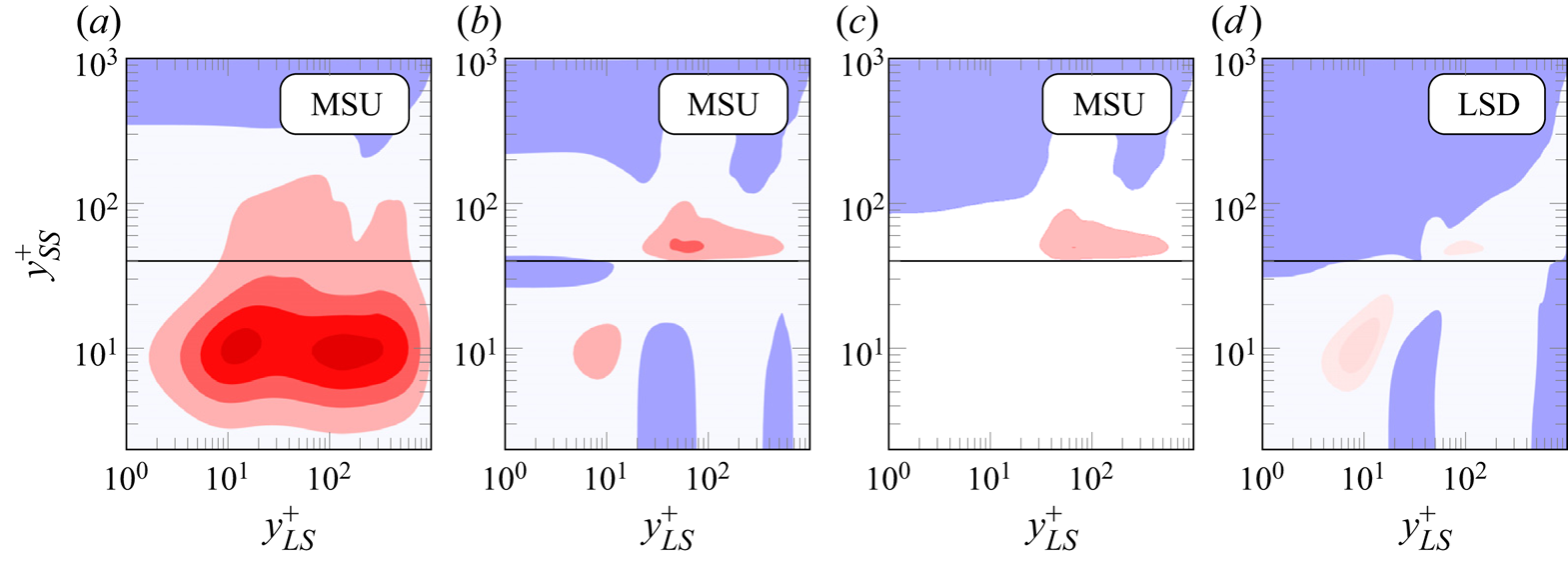
Figure 12. Plots of  $C_{{AM}}^\ast$ maps with a modified threshold wavelength $\lambda _{z,c}^+ = 1000$. (a) Reference, unperturbed MSU case. (b,c) MSU with suppression of modulation, where in (c), the modulating effects given by mode $\kappa _z = 0$ have been removed. (d) LSD with suppression of modulation. The modulation-suppressing forcing is active on small scales at $y_{SS}^+ \leqslant 40$; the boundary of this region is marked with a black line. Colour map and levels as in figure 5 except for (d), for which colour levels are $(-0.5; 0; 0.18; 0.25)$.
Having confirmed that the  $C_{{AM}}^\ast$ map behaves as expected, the focus is now turned to the main result of interest for this case – that is, energy spectra. These are shown in figure 13 for the MSU and LSD cases with suppression of modulation; the boundaries of the region where the suppression is active are marked by a solid black line. As expected, spectra exhibit a striped pattern in this region, alternating single, extremely excited modes with depressed regions corresponding to suppressed modes. Interestingly, the striped pattern is also observed further away from the wall where the forcing is not active, in what seems to be a bottom-up effect; at the same time, modes that were previously suppressed are now free to develop in this area, contributing to the unusual secondary peak in $\left \langle {u'u'} \right \rangle$ seen in figure 11. To recover a meaningful spectrum from the observed striped pattern, the smoothing technique described in § 2.3 is used; results are shown in figures 13(c,d). It is revealed that the striped pattern hides a small-scale buffer-layer peak typical of wall-bounded turbulence, which is (at least qualitatively) captured correctly. Although near-wall small scales are being targeted by the forcing, their corresponding values of the spectrum are increased with respect to the unperturbed simulations (see figure 5 for comparison). Instead, near-wall large scales of the forced simulations show unusually low energy, as will be discussed below; overall, the increase in small-scale energy dominates, so that excess energy is seen on the streamwise fluctuations in the near-wall region (as observed in the $\left \langle {u'u'} \right \rangle$ profiles of figure 11). Large scales in the core of the channel are captured reasonably correctly also in presence of the forcing, indicating that these can exist in the absence of near-wall modulation; this once again corroborates the idea that outer layers are autonomous (Flores & Jiménez Reference Flores and Jiménez2006; Mizuno & Jiménez Reference Mizuno and Jiménez2013; Kwon & Jiménez Reference Kwon and Jiménez2021).

Figure 13. Premultiplied spanwise spectrum  $\kappa _z^+\phi _{uu}^+$ of the streamwise fluctuation. (a,b) LSD and MSU cases with suppression of modulation; (c,d) same cases, with the spectrum being smoothed as explained in § 2.3. The boundaries of the region where the forcing is active are marked with a solid black line. Colour map as in figure 5.
The reduction of the near-wall large-scale energy content of figure 13(b) (for instance) with respect to the unperturbed case (figure 5b) cannot be explained trivially; these scales are indeed not affected directly by the forcing. At  $(y^+,\lambda _z^+) \approx (10.2, 1750)$, an $87\,\%$ reduction in the value of $\phi _{uu}^+$ is observed. This might be interpreted as the absence of superposition phenomena, possibly suggesting that superposition might in fact be enhanced by large-scale modulation of the amplitude of the small scales. The above conjecture is supported by evidence of a small- to large-scale power transfer in the buffer layer of wall-bounded flows observed, for instance, by Cho et al. (Reference Cho, Hwang and Choi2018), Andreolli, Quadrio & Gatti (Reference Andreolli, Quadrio and Gatti2021) and Chiarini et al. (Reference Chiarini, Mauriello, Gatti and Quadrio2022). Exploiting a generalised quasi-linear approximation of a turbulent channel flow, Hernández, Yang & Hwang (Reference Hernández, Yang and Hwang2022) also support the idea that small-scale fluctuations may be involved in large-scale generation mechanisms. They found that the inhibition of particular triadic interactions involved in inverse energy transfer in the spanwise direction within the near-wall region led to suppression of the near-wall positive turbulent transport at large scales. However, we deem the suppression technique employed here too intrusive to make a firm statement: another possible explanation for the lack of energy from near-wall large scales could be that all the near-wall large-scale activity is lumped into the Fourier mode with $\lambda _z^+ \approx 1000$, for which the spectrum shows an unusually high value.
4. Conclusions
In the present work, we performed and analysed numerical simulations in which either the superposition of the large scales at the wall or amplitude modulation of the near-wall small scales was suppressed thanks to purposely designed body forces. Both standard, long streamwise domains (LSDs) and minimal streamwise unit (MSU) domains have been used; no qualitative difference between the two has been observed in the results, although quantitative differences do arise. This suggests that MSUs can capture the fundamental mechanisms of the investigated scale interactions; a similar conclusion was drawn by Kawata & Tsukahara (Reference Kawata and Tsukahara2021). Streamwise-elongated structures that are longer than the computational box of the MSU will be represented in such restricted domains as streamwise-invariant (Toh & Itano Reference Toh and Itano2005); the lifetime of these structures in an MSU reflects their streamwise extent in an LSD (Abe et al. Reference Abe, Antonia and Toh2018). Therefore, we expect the large scales of an MSU to modulate the amplitude of the small ones in the spanwise direction and in time; this is indeed what we observe.
Our findings concerning the scale interactions are summarised in figure 14. Suppression of superposition means that large scales are removed from the near-wall region. In the absence of the near-wall large scales, it is revealed that the amplitude of the buffer-layer small scales still correlates well with the outer-layer large ones. According to some studies (for instance, Ganapathisubramani et al. Reference Ganapathisubramani, Hutchins, Monty, Chung and Marusic2012; Zhang & Chernyshenko Reference Zhang and Chernyshenko2016; Agostini & Leschziner Reference Agostini and Leschziner2019a), the removed large scales cause the amplitude modulation (AM) of the small scales; this is depicted schematically in figure 14 by a grey line. However, it is self-evident that the correlation that we observe currently cannot be explained as an effect of the superposed large scales, or of the large-scale gradient at the wall or in its proximity, as these have been removed. Hence amplitude modulation should be understood not as a local modulation mechanism, but rather as a correlation of the amplitude of the small scales in the buffer layer with large scales from several wall-normal positions, represented in figure 14 by a black line. Other authors have linked scale interactions to the circulatory congregative and dispersive motions induced at the wall by log-layer sweeps and ejections (for instance, Toh & Itano Reference Toh and Itano2005; Hwang et al. Reference Hwang, Lee, Sung and Zaki2016). Since the superposition removal affects all velocity components, our results also challenge the theory of Toh & Itano (Reference Toh and Itano2005): in the absence of near-wall large scales, there cannot be any spanwise large-scale wind transporting near-wall streaks towards large-scale ejections as proposed by the authors. Moreover, it is unclear how the large-scale circulatory structure associated with log-layer sweeps and ejections, observed for instance by Hwang et al. (Reference Hwang, Lee, Sung and Zaki2016), would penetrate to the wall as it normally does.

Figure 14. A schematic representation of the widely accepted scale interaction mechanism (grey arrows) and our observations (black).
Suppression of modulation is performed near the wall by making modulation non-representable in the spectral simulation domain, more precisely by damping selected small-scale spanwise Fourier modes. In addition to blocking modulation, this forcing prevents the interaction between small-scale modes resulting in a transfer of energy to large scales; moreover, triadic interactions between small and large modes are blocked indirectly. Interestingly, this forcing significantly affects the mean velocity profile, as the produced flow rate is substantially increased at constant pressure gradient. Also, near-wall large-scale modes seem to vanish, indicating that these might receive a significant amount of energy from the interaction of near-wall small-scale modes, rather than from a top-down footprinting effect; this idea is reported schematically in figure 14 as a black line.
While the latter observation is in line with the evidence of a small-to-large energy transfer in the near-wall region found by Cho et al. (Reference Cho, Hwang and Choi2018), Jacobi et al. (Reference Jacobi, Chung, Duvvuri and McKeon2021) and Hernández et al. (Reference Hernández, Yang and Hwang2022), the results yielded by suppression of superposition show that the present understanding of amplitude modulation is still only partial. Our results do not exclude that, for instance, the large-scale velocity gradient may locally have a modulating action on small-scale activity as proposed by Agostini & Leschziner (Reference Agostini and Leschziner2019a); moreover, the ansatz that near-wall small scales are locally modulated by near-wall large scales (for instance, Zhang & Chernyshenko Reference Zhang and Chernyshenko2016) can still be a starting point for models that yield satisfactory results, owing to the spatial coherence of the large scales. Nevertheless, our data indicate that a local mechanism involving near-wall large scales can only partially explain the correlation commonly known as amplitude modulation.
Acknowledgements
The authors acknowledge support from the state of Baden-Württemberg through bwHPC. This work was performed with the help of the Large Scale Data Facility of at the Karlsruhe Institute of Technology funded by the Ministry of Science, Research and the Arts Baden-Württemberg, and by the German Federal Ministry of Education and Research.
Funding
This work is supported by the Priority Programme SPP 1881 Turbulent Superstructures of the Deutsche Forschungsgemeinschaft (D.G. and A.A.; grant no. GA 2533/1-1). We also gratefully acknowledge funds provided by the Lundeqvist foundation.
Declaration of interests
The authors report no conflict of interest.
Author contributions
D.G., P.S., R.Ö. and R.V. contributed to the original idea of the paper. D.G. and A.A. implemented and performed the simulations and analysis techniques, as well as writing the first draft. All authors contributed equally to analysing data and reaching conclusions, and to revising the draft.
Appendix
The spanwise co-spectra of the Reynolds shear stress are shown in figure 15 for all forced and unforced cases in both the LSD and MSU domains. The co-spectra of the unperturbed cases (figures 15a,e) show an elongated peak that extends from near-wall small scales to large scales in the outer layer; this qualitative structure is retained by the simulations with suppression of superposition and with suppression of modulation.

Figure 15. Co-spectra of  $-\left \langle {u'v'} \right \rangle$ for the LSD and MSU simulations. (a,e) Reference cases without forcing. (b,f) Cases with suppression of superposition (c,d,g,h) Cases with suppression of modulation, where in (d,h) the smoothed co-spectrum defined in § 2.3 is shown.
In the simulation with suppression of superposition, large-scale motions are removed from the proximity of the wall; the contour of the suppressed region is marked with a black line in figures 15(b,f). In the reference cases (figures 15a,e), the values of the co-spectrum are negligibly low in this region, meaning that large-scale near-wall sweeps and ejections contribute only marginally to the profile of the Reynolds shear stress. As expected, their removal proves to be rather unintrusive in figures 15(b,f); the only noticeable difference with figures 15(a,e) is that suppressed modes are somewhat weakened by the suppressing action at the wall, even at a distance from it. This results in a slight distortion of the bottom border of the spectral  $\left \langle {u'v'} \right \rangle$ peak.
As for the simulation with suppression of modulation, the co-spectra of figures 15(c,g) show the usual striped pattern associated with this forcing (see figure 13). Figures 15(d,h) show the same spectrum by smoothing it with the procedure described in § 2.3. This yields a qualitatively correct co-spectrum that resembles the one of figures 15(a,e), albeit with minor distortions. Unlike the spectrum of streamwise fluctuations (figure 13), no particular increase (or decrease) of the values of the co-spectrum is seen with respect to the reference case.


 Open access