


1. Introduction
Turbulent particle-laden flows are of relevance to many engineering applications such as gas turbine engine combustors used for aircraft propulsion, cyclones used for particle separation, industrial driers and slurry pumps, see the works of Crowe et al. (Reference Crowe, Schwarzkopf, Sommerfeld and Tsuji2011), Kuerten (Reference Kuerten2016) and Zhao et al. (Reference Zhao, Zhao, Zhang, Li and Geng2021). Thus, several theoretical, numerical and experimental investigations have been carried out over the past decades, and many review papers have been published, see for example those of Poelma & Ooms (Reference Poelma and Ooms2006), Balachandar & Eaton (Reference Balachandar and Eaton2010) and Brandt & Coletti (Reference Brandt and Coletti2022). Review of these studies suggests that, among many non-dimensional parameters, the Stokes number (which is the ratio of particle to flow time scale, as defined by, for example, Crowe et al. Reference Crowe, Schwarzkopf, Sommerfeld and Tsuji2011) primarily influences the characteristics of the turbulent particle-laden flows. Although past investigations are of significant importance as they provide insight into relatively small and moderate Stokes number flows ( $St\lesssim 10$), the Stokes number of particle-laden flows relevant to some engineering applications such as sprays in gas turbine engine combustors, is relatively large (
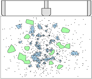
 $St \gtrsim 10$). The present study is motivated by the need for understanding the spray characteristics at relatively large Stokes numbers. As elaborated by Baker et al. (Reference Baker, Frankel, Mani and Coletti2017) and Boddapati, Manish & Sahu (Reference Boddapati, Manish and Sahu2020), the interaction of the particles and the background turbulent flow leads to the formation of regions with relatively large and small number of particles, which are referred to as clusters and voids, respectively, and are relevant to the present study. A brief review of the literature related to the clusters and voids is provided below.
The inertial bias and sweep-stick mechanisms are proposed in the literature to elaborate the formation of clusters and voids in turbulent flows. The former suggests that during a particle and eddy interaction, the large eddies centrifuge out the particles and accumulate them in regions that feature small vorticities and large strain rates, as explained by Maxey (Reference Maxey1987), Squires & Eaton (Reference Squires and Eaton1991) and Wang & Maxey (Reference Wang and Maxey1993). Compared with the inertial bias mechanism, the sweep-stick mechanism suggests that the vorticity and strain rate fields may not be sufficient in explaining the positioning of the particles and hence formation of the clusters, see the work of Goto & Vassilicos (Reference Goto and Vassilicos2008). The sweep-stick mechanism suggests that particles with  $St \gtrsim 1$ tend to be positioned in the spatial locations with zero acceleration. Then, these particles are carried by large eddies in the flow, see the works of Goto & Vassilicos (Reference Goto and Vassilicos2006), Monchaux, Bourgoin & Cartellier (Reference Monchaux, Bourgoin and Cartellier2012), Mora et al. (Reference Mora, Bourgoin, Mininni and Obligado2021) and Hassaini & Coletti (Reference Hassaini and Coletti2022).
Various tools and methods have been developed to identify the clusters and voids from the spatial distribution of the particles. For example, Monchaux, Bourgoin & Cartellier (Reference Monchaux, Bourgoin and Cartellier2010), Tagawa et al. (Reference Tagawa, Mercado, Prakash, Calzavarini, Sun and Lohse2012) and Frankel et al. (Reference Frankel, Pouransari, Coletti and Mani2016) utilized the Voronoï cells, Andrade, Hardalupas & Charalampous (Reference Andrade, Hardalupas and Charalampous2022) used the combined graph and Voronoï cells, Fessler, Kulick & Eaton (Reference Fessler, Kulick and Eaton1994) and Villafañe-Roca et al. (Reference Villafañe-Roca, Esmaily-Moghadam, Banko and Eaton2016) implemented the box-counting method, and Salazar et al. (Reference Salazar, De Jong, Cao, Woodward, Meng and Collins2008), Saw et al. (Reference Saw, Shaw, Ayyalasomayajula, Chuang and Gylfason2008) and Sahu, Hardalupas & Taylor (Reference Sahu, Hardalupas and Taylor2016) applied the radial distribution functions to identify the clusters. The Voronoï cells (relevant to the present investigation) can allow for estimating the degree of clustering, which is defined (see for example Boddapati et al. Reference Boddapati, Manish and Sahu2020) as the root mean square (RMS) of the normalized Voronoï cells area ( $\sigma$) divided by that if the droplets were distributed following a random Poisson process (RPP), $\sigma _{\rm RPP}$, minus unity. The studies of Monchaux et al. (Reference Monchaux, Bourgoin and Cartellier2010), Obligado et al. (Reference Obligado, Teitelbaum, Cartellier, Mininni and Bourgoin2014) and Sumbekova et al. (Reference Sumbekova, Cartellier, Aliseda and Bourgoin2017) showed that the degree of clustering is influenced by three non-dimensional parameters that are the Stokes number ( $St$) estimated based on the Kolmogorov time scale, Taylor-length-scale-based Reynolds number ( $Re_\lambda$) and the droplets volume fraction ( $\phi _{{\rm v}}$). Monchaux et al. (Reference Monchaux, Bourgoin and Cartellier2010) and Obligado et al. (Reference Obligado, Teitelbaum, Cartellier, Mininni and Bourgoin2014) showed that for relatively small values of the Stokes number ( $St \lesssim 10$) and for relatively small values of the Taylor-length-scale-based Reynolds number ( $Re_\lambda \lesssim 200$), the degree of clustering increases by increasing the Stokes number and maximizes at $St\approx 2\unicode{x2013}4$. Further increasing the Stokes number decreases the degree of clustering. Compared with those of Monchaux et al. (Reference Monchaux, Bourgoin and Cartellier2010) and Obligado et al. (Reference Obligado, Teitelbaum, Cartellier, Mininni and Bourgoin2014), the study of Sumbekova et al. (Reference Sumbekova, Cartellier, Aliseda and Bourgoin2017) showed that, for relatively small values of the Stokes number but relatively large values of the Taylor-length-scale-based Reynolds number ( $Re_\lambda \gtrsim 200$), $St$ does not greatly influence the degree of clustering, however, this parameter scales with $Re_\lambda$ and the square root of $\phi _{{\rm v}}$. The studies of Sumbekova et al. (Reference Sumbekova, Cartellier, Aliseda and Bourgoin2017), Obligado et al. (Reference Obligado, Teitelbaum, Cartellier, Mininni and Bourgoin2014) and Monchaux et al. (Reference Monchaux, Bourgoin and Cartellier2010) showed that the probability density function (PDF) of the cluster and void areas feature power-law correlations with the exponents of the power-law ranging from approximately $-$1.5 to $-$2.1 and $-$1.7 to $-$1.9, respectively. Sumbekova et al. (Reference Sumbekova, Cartellier, Aliseda and Bourgoin2017) showed that the PDFs of the cluster and void areas normalized by their corresponding mean value feature a power-law decay with an exponent of $-$5/3 for normalized cluster and void areas ranging from approximately 0.2 to 10.
In addition to the PDFs of the cluster and void areas, the length scales of the clusters and voids and how they relate the length scales of the turbulent flow have been studied. The characteristic length scales of the clusters and voids are defined as the square root of the cluster and void mean areas, respectively. The studies of Aliseda et al. (Reference Aliseda, Cartellier, Hainaux and Lasheras2002), Obligado et al. (Reference Obligado, Teitelbaum, Cartellier, Mininni and Bourgoin2014), Sumbekova et al. (Reference Sumbekova, Cartellier, Aliseda and Bourgoin2017), Sahu et al. (Reference Sahu, Hardalupas and Taylor2016) and Boddapati et al. (Reference Boddapati, Manish and Sahu2020) showed that the cluster length scale is approximately 5–90 times the Kolmogorov length scale. For voids, Sumbekova et al. (Reference Sumbekova, Cartellier, Aliseda and Bourgoin2017) showed that the length scale can increase to approximately 200 times the Kolmogorov length scale. Power-law formulations were developed by Sumbekova et al. (Reference Sumbekova, Cartellier, Aliseda and Bourgoin2017) and it was shown that the normalized cluster length scale is proportional to  $St^{-0.25}Re_\lambda ^{4.7}\phi _{{\rm v}}^{1.2}$. Also, Sumbekova et al. (Reference Sumbekova, Cartellier, Aliseda and Bourgoin2017) showed that, despite the Stokes number does not significantly influence the normalized voids length scale, this positively relates to $Re_\lambda$ and $\phi _{{\rm v}}$.
Although the generated knowledge from the particle-laden flow studies (with a brief review presented above) is of significant importance, as it allows to understand the clustering characteristics of droplets corresponding to relatively small Stokes numbers ( $St < 10$), some engineering application feature droplets with large Stokes numbers. In such applications, it is of significant importance to understand the distribution of the droplet diameter and their number density within a given cluster and for $St > 10$. For example, for spray combustion-related applications (which feature Stokes numbers in excess of 10), the mean distance between the fuel droplets and their number density within a given cluster can influence the droplet evaporation rate as well as the flame location and the temperature distribution, see for example the works of Sahu, Hardalupas & Taylor (Reference Sahu, Hardalupas and Taylor2018), Hardalupas, Taylor & Whitelaw (Reference Hardalupas, Taylor and Whitelaw1994), Akamatsu et al. (Reference Akamatsu, Miutani, Katsuki, Tsushima and Cho1996), Pandurangan & Sahu (Reference Pandurangan and Sahu2022) and Weiss et al. (Reference Weiss, Bhopalam, Meyer and Jenny2021). The objective of the present study is to investigate the effect of the Stokes number on both the geometrical (e.g. clusters and voids length scales) as well as the joint characteristics of the droplets and clusters/voids for $St > 10$. In the following, the methodology, data reduction, results and concluding remarks are presented in §§ 2–5, respectively.
2. Experimental methodology
The experimental set-up, the utilized diagnostics and the tested conditions are presented in this section.
2.1. Experimental set-up
The experimental set-up consists of a liquid delivery and flow apparatuses, which are shown in figure 1 as items (1–3) and item (4), respectively. A nitrogen bottle, item (1) in the figure, as well as a dual-valve MCRH 2000 ALICAT pressure controller, item (2), were used to purge water inside a pressure vessel, item (3). Then, water flowed into the flow apparatus, see the blue arrow in figure 1. In addition to water, a compressor was used to provide air into the flow apparatus, see the black arrow in figure 1. The air flow rate was controlled using an MCRH 5000 ALICAT mass flow controller.

Figure 1. Experimental set-up. Items (1–3) are a nitrogen bottle, a pressure controller and a pressurized water vessel. Item (4) is the nozzle section of the flow apparatus. Item (5) is a 532 nm Nd:YAG laser. Items (6–8) are the laser sheet forming optics and optomechanics. Items (9) and (10) are a Nova S12 camera and lens as well as a Zyla camera and lens for simultaneous Mie scattering and interferometric laser imaging for droplet sizing (ILIDS) measurements.
The flow apparatus is composed of a diffuser section (with an area ratio of 4), a settling chamber (which is equipped with five equally spaced mesh screens), a contraction section (with an area ratio of 7) and a nozzle (with an inner diameter of 48.4 mm). Further details regarding the apparatus are provided by Mohammadnejad, Saca & Kheirkhah (Reference Mohammadnejad, Saca and Kheirkhah2022), Kheirkhah & Gülder (Reference Kheirkhah and Gülder2015) and Kheirkhah (Reference Kheirkhah2016). The nozzle section of the flow apparatus is shown in figure 2. In the present study, this section was modified to allow for producing a spray subjected to turbulent co-flow of air. The nozzle includes a 6.4 mm outer diameter tube (which carries water), a spray injector, a turbulence generation mechanism and a ring-shaped tube-holder, which was press-fit against the inner wall of the nozzle and the outer wall of the tube using four bars and a collar. The injector was a pressure swirl atomizer from Delavan (model 6330609), which produced a polydisperse spray. The spray flow rate depends on the vessel pressure, and separate calibration experiments were performed to obtain the relation between the vessel pressure and the spray flow rate, as discussed in Appendix A.

Figure 2. (a) and (b) Three-dimensional (3-D) drawing of the flow apparatus nozzle section for the second and third turbulence generation mechanisms, respectively.
Three turbulence generation mechanisms were used in the present study. Either no perforated plate, one perforate plate (see figure 2a) or two perforated plates attached back-to-back (see figure 2b) were utilized. The outer diameter of each perforated plates is 48.4 mm, matching the inner diameter of the nozzle. Each perforated plate features 3.9 mm diameter holes arranged in a hexagonal pattern. For the first turbulence generation mechanism, the perforated plates in figure 2 were removed. For the third turbulence generation mechanism, the plates were rotated by 60 $^{\circ }$ with respect to one another, similar to that in the study of Kheirkhah & Gülder (Reference Kheirkhah and Gülder2014). For the second turbulence generation mechanism, the planes containing the holes, and for the third turbulence generation mechanism, the centre plane of the two perforated plates, were positioned 76.0 mm upstream of the nozzle exit plane, similar to the studies of Kheirkhah & Gülder (Reference Kheirkhah and Gülder2015) and Kheirkhah (Reference Kheirkhah2016).
2.2. Diagnostics
Separate hotwire anemometry (HWA) as well as simultaneous Mie scattering and interferometric laser imaging for droplet sizing (ILIDS) were performed. The hotwire anemometry was used to characterize the background turbulent flow. A schematic of the diagnostics used in the present study is shown in figure 1. The hardware configuration for the HWA is identical to that used by Mohammadnejad et al. (Reference Mohammadnejad, Saca and Kheirkhah2022); so a separate illustration is not presented in figure 1. For all test conditions, the HWA data were acquired at a frequency of 100 kHz and for 90 s, corresponding to 9 000 000 data points. The simultaneous Mie scattering and ILIDS images were collected at a frequency of 10 Hz and for a duration of 80 s, corresponding to 800 image pairs. Further details regarding the HWA, Mie scattering and ILIDS diagnostics are provided in the following.
2.2.1. Hotwire anemometry
The hardware of the HWA system consists of a probe (model 55P01 from Dantec), a probe support (model 9055H0261 from Dantec) and two motorized translational stages (MTS50-Z8 from Thorlabs). The probe is a single wire sensor, which is 3 mm long (with an active sensor length of 1.25 mm) and has a diameter of 5  $\mathrm {\mu }$m. A mini-constant temperature anemometry (mini-CTA) circuit (model 9054T0421 from Dantec) maintains the wire temperature, with an overheat ratio of 0.7. The motorized translational stages featured a 50 mm range of operation, which was sufficient for the present study. Further details regarding the HWA system as well as the calibration procedure are provided by Mohammadnejad et al. (Reference Mohammadnejad, Saca and Kheirkhah2022).
A Cartesian coordinate system was used in the present investigation. The origin of the coordinate system is at the exit plane of the nozzle section and at the nozzle centreline, as shown in figure 3. The  $z$-axis coincides with the nozzle centreline. The $x$-axis is normal to the $z$-axis and is parallel with the laser sheet shown in figure 1. HWA was performed at $z = 35.0$ mm and at horizontal locations spaced by 5.0 mm along the $x$-axis, ranging from $x = -20.0$ to 20.0 mm as shown by the red cross data symbols in figure 3.

Figure 3. Coordinate system and the measurements locations. The red cross data points present the locations at which the hotwire anemometry was performed. The dashed black and dash–dotted blue squares are the regions of interest for the Mie scattering and ILIDS measurements, respectively. The minimum vertical distance for the above measurements is 35.0 mm from the nozzle exit plane, and this distance shown in the figure is not to scale.
2.2.2. Mie scattering
The Mie scattering hardware consists of a pulsed Nd:YAG laser (Lab-Series-170 from Spectra Physics, shown by item (5) in figure 1), the sheet forming optics (see items (6–8)) and a camera equipped with collection optics (item (9)). The laser produces a 1064 nm beam, which is converted to a 532 nm beam using a harmonic generator. The laser was operated at a reduced (compared to its maximum) but fixed energy to avoid saturation in the collected Mie scattering images. The laser beam was 8.0 mm in diameter, which was converted to a 40 mm high and 1 mm thick laser sheet using a plano-concave cylindrical lens with a focal length of  $-$100 mm, a plano-convex cylindrical lens with a focal length of 500 mm and a cylindrical lens with a focal length of 1000 mm, see items (6–8) in figure 1. The centreline of the collimated laser sheet was positioned at $z=55.0$ mm. The Mie scattering images were acquired using a Photron Fastcam Nova S12 camera equipped with a Macro Sigma lens, which had a focal length of $f =105$ mm and its aperture size was set to $f/2.8$. A bandpass filter with a centre wavelength and full width at half maximum of 532 and 20 nm was mounted on the camera lens. By adjusting the working distance of the camera, a field of view of 70.0 mm along the $x$-axis and 70.0 mm along the $z$-axis was obtained, which corresponds to a pixel resolution of $70\,\mathrm {mm}/1024\,\mathrm {pixels}=68\,\mathrm {\mu }\mathrm {m}\,\mathrm {pixel}^{-1}$. For analysis and presentation purposes, the above field of view was cropped to a $50.0\,{\rm mm}\times 50.0\,{\rm mm}$ square, which is shown by the black dashed box in figure 3. It is noted that since the above field of view is close to the injector, the air entrainment may occur and the background turbulent air flow may be anisotropic. A field of view that is located farther from the injector could facilitate reducing the effect of the air entrainment into the spray on the reported results and/or improve the background turbulent flow isotropy. However, the present study employed an injector that is used for reacting flow applications for which the majority of the turbulence and droplet interaction takes place close to the injector. In fact, at distances larger than 85 mm and for reacting conditions (not discussed here), the droplets are evaporated, burned and do not exist. For this reason, a field of view that is close to the injector is chosen. At distances smaller than 35 mm, the spray was too dense and the images were influenced by the laser reflection from the injector; as a result, the analysis of the Mie scattering images was not feasible.
2.2.3. Interferometric laser imaging for droplet sizing
ILIDS was performed to measure the droplets diameter, similar to that done by Qieni et al. (Reference Qieni, Kan, Baozhen and Xiang2016), Bocanegra Evans et al. (Reference Bocanegra Evans, Dam, van der Voort, Bertens and van de Water2015) and Garcia-Magarino et al. (Reference Garcia-Magarino, Sor, Bardera and Munoz-Campillejo2021). In ILIDS, the droplet diameter is measured by analysing the interference pattern of the reflected and first-order refracted rays scattered from spherical droplets that are illuminated by a laser. The ILIDS hardware includes the laser and the laser-sheet forming optics, see items (5–8) in figure 1, which are identical to those used for the Mie scattering technique as well as a scientific complementary metal-oxide semiconductor (sCMOS) camera equipped with a Macro sigma lens ( $\,f = 105$ mm and aperture size of $f/2.8$) and a high-precision rotary stage, see item (10). The camera is a 5.5 Zyla from Andor, which has a $2560\,{\rm pixels}\times 2160\,{\rm pixels}$ sensor. The ILIDS field of view was 29.4 mm along the $x$-axis and 24.6 mm along the $z$-axis, which led to a pixel resolution of $29.4\,\mathrm {mm}/2560\,\mathrm {pixels} = 11.4\,\mathrm {\mu }\mathrm {m}\,\mathrm {pixel}^{-1}$. Using the rotary stage, the angle between the axis normal to the camera sensor and the direction of the laser sheet, $\theta$, was adjusted. Sahu (Reference Sahu2011) utilized the Mie scattering theory and obtained the variations of the intensities of the first-order refraction and reflected light versus the scattering angle for water droplets. For these droplets, they showed that the above intensities are equal at approximately $\theta =69^{\circ }$, creating interference patterns with a maximized amplitude which leads to the best clarity of the fringe patterns. In the present study, and similar to those performed by Sahu (Reference Sahu2011) and Sahu et al. (Reference Sahu, Hardalupas and Taylor2016), $\theta$ was set to 69 $^{\circ }$. Finally, the formulation by Hayashi, Ichiyanagi & Hishida (Reference Hayashi, Ichiyanagi and Hishida2012) and Thimothée et al. (Reference Thimothée, Chauveau, Halter and Gökalp2016) was used to estimate the droplet diameter, which is given by
 \begin{equation} d=\frac{2\lambda_\mathrm{L} N}{\alpha}\left[\cos\left(\frac{\theta}{2}\right)+ \frac{m\sin\left(\dfrac{\theta}{2}\right)}{\sqrt{m^{2}-2m\cos\left(\dfrac{\theta}{2}\right)+1}}\right]^{{-}1}, \end{equation}
where  $\lambda _{{\rm L}}$ is the wavelength of the laser and is 532 nm. In (2.1), $m$ is the droplets index of refraction, which equals 1.33 for water, and $\alpha$ is the collection angle of the scattered light. The collection angle depends on the utilized lens diameter ( $d_{{\rm l}}$, which is 60 mm), and the distance between the camera lens and the projected location of the droplets in the measurement plane ( $c$). Specifically, the collection angle is calculated using $\alpha =2\arctan [d_{{\rm l}}/(2c)]$. In the present study, while $d_{{\rm l}}$ is fixed, $c$ can vary from 195 to 205 mm. Thus, the collection angle is not constant across the image plane. Here, a fixed value of $c = 200$ mm was used which can lead to an error in the calculation of the droplet diameter. This error was quantified, and it was obtained that the maximum error due to the variation of $c$ is less than 2.5 %.
In (2.1),  $N$ is the number of the fringes and is estimated using the procedure discussed in the next section. Substituting $N=1$ and the values of $\lambda _{{\rm L}}$, $m$,
$m$,  $\theta$ and $\alpha$ in (2.1), the droplet diameter per fringe is obtained, which is 1.97 $\mathrm {\mu }$m. Since at least two fringes are required for the detection of the droplets, the minimum measurable diameter of the droplets is twice the diameter per fringe which is $2\times 1.97\,\mathrm {\mu }{\rm m} \approx 4\,\mathrm {\mu }$m. Also, considering the widths of the fringes, the maximum resolvable diameter is estimated and equals 150 $\mathrm {\mu }$m. Challenges exist in performing simultaneous ILIDS and Mie scattering measurements as well as interpreting the results, which need to be addressed. Since the viewing angle of the ILIDS camera is different than that of the Mie scattering camera, simultaneous measurement of the location of the droplets using the Mie scattering and ILIDS techniques require registering the ILIDS images to the Mie scattering images. Even after the registration of the ILIDS image to the Mie scattering image, since the ILIDS images are out-of-focus, the centres of the droplets identified from the ILIDS images are not identical to those obtained form the Mie scattering images. Furthermore, due to the limitations of the ILIDS technique, the number of droplets detected in each frame of the ILIDS does not equate to that of the Mie scattering technique. The above potentially lead to uncertainty in estimating the joint characteristics of the droplets and clusters/voids. Details for addressing/assessing the issues related to the droplets centre discrepancy and average diameter uncertainty for the calculation of the joint characteristics are discussed in Appendices B and C, respectively.
2.3. Test conditions
In total, 13 experimental conditions were tested, with the corresponding details tabulated in table 1. The first row in the table highlights the test condition for which no co-flow is used and the spray is issued into the quiescent air. The first column in the table presents the utilized turbulence generation (TG) mechanism, with 0PP, 1PP and 2PP referring to zero, one and two perforated plates, respectively. For each turbulence generation mechanism, the mean bulk flow velocities of 3.5, 7.0, 10.5 and 14.0 m s $^{-1}$ were tested. The bulk Reynolds number was calculated using $Re_{D}=UD/\nu$, with $D$ being the nozzle diameter and $\nu$ being the air kinematic viscosity estimated at the laboratory temperature. The values of $Re_D$ are tabulated in the third column of table 1. The RMS of the streamwise velocity ( $u'_0$) and the integral length scale ( $\varLambda$) estimated at $x=0$ and $z = 35.0$ mm are listed in the fourth and fifth columns of table 1, respectively. The integral length scale was calculated using the Taylor's frozen turbulence hypothesis, see the work of Taylor (Reference Taylor1938), and following the procedure detailed by Mohammadnejad et al. (Reference Mohammadnejad, Saca and Kheirkhah2022). Specifically, the integral length scale was calculated as the multiplication of the mean bulk flow velocity and the integral of the streamwise velocity auto-correlation from $t=0$ to the first time that the auto-correlation becomes zero. The Taylor ( $\lambda$) and Kolmogorov ( $\eta$) length scales were calculated using $\lambda = \varLambda (u^\prime _0 \varLambda /\nu )^{-0.5}$ and $\eta = \varLambda (u^\prime _0 \varLambda /\nu )^{-0.75}$. The values of $\lambda$ and $\eta$ are tabulated in the sixth and seventh columns of table 1. For all test conditions, the most probable droplet diameters ( $d^*$) were obtained using the ILIDS diagnostic and are listed in the eighth column of the table. Further details regarding the size distribution of the droplets are discussed in § 4.1.
Table 1. Test conditions. TG stands for the turbulence generating mechanism. 0PP, 1PP and 2PP are the acronyms for zero, one and two perforated plates, respectively.

The Taylor-length-scale-based Reynolds number, the Stokes number and the liquid volume fraction are non-dimensional parameters that can potentially influence the interaction of the droplets with the background turbulent flow. The Taylor-length-scale-based Reynolds number was estimated using  $Re_\lambda = u^\prime _0 \lambda /\nu$, with the corresponding values listed in the ninth column of table 1. In the present study, $Re_\lambda$ varies from approximately 10 to 36, which corresponds to relatively small values. Following Reade & Collins (Reference Reade and Collins2000), the Stokes number was calculated using
 \begin{equation} St=\frac{1}{18}\frac{\rho_{{\rm W}}}{\rho_{{\rm A}}}\left(\frac{d}{\eta}\right)^2, \end{equation}
where  $\rho _{{\rm W}}$ and $\rho _{{\rm A}}$ are the water and air densities, respectively, both estimated at the laboratory temperature. In (2.2), $d$ is the droplet diameter. In the present study, $d$ was selected as the most probable droplet diameter for estimation of the Stokes number, with the rationale for this selection discussed later. The values of $St$ are tabulated in table 1 and range from approximately 3 to 25, which are relatively large compared to those of the studies that were performed in multi-phase wind tunnels. It is worth highlighting that, in addition to the most probable droplet diameter, the Sauter mean diameter was also estimated for all test conditions following the formulation given by Lefebvre & McDonell (Reference Lefebvre and McDonell2017). The Stokes number estimated based on the Sauter mean diameter and the Kolmogorov length scale varied from 17 to 150 and positively correlated with the Stokes number estimated based on the most probable droplet diameter and the Kolmogorov length scale. Additionally, instead of the Kolmogorov length scale, the Stokes number was also estimated based on the integral length scale. It was obtained that the Stokes numbers estimated based on both length scales positively correlate. Given the above correlations, presentation of the results using the Stokes number estimated based on either of the length scales or either of the diameters yielded similar conclusions. Nonetheless, facilitating comparisons with the past investigations, e.g. those of Sumbekova et al. (Reference Sumbekova, Cartellier, Aliseda and Bourgoin2017), Obligado et al. (Reference Obligado, Teitelbaum, Cartellier, Mininni and Bourgoin2014) and Monchaux et al. (Reference Monchaux, Bourgoin and Cartellier2010), the Stokes number estimated based on the most probable droplet diameter and the Kolmogorov length scale was used in the discussions and analyses.
Following the definition provided by Elghobashi (Reference Elghobashi1994), the liquid volume fraction was calculated from
 \begin{equation} \phi_{{\rm v}} = n\frac{V_{{\rm d}}}{V_{{\rm ROI}}}, \end{equation}
where  $n$ is the mean number of droplets within the volume of the region of interest (ROI), $V_{{\rm ROI}}$. In (2.3), $V_{{\rm d}}$ is the droplet volume. For each test condition, $n$ was estimated using the Mie scattering technique and averaged over all collected Mie scattering images. $V_{{\rm ROI}} = 50\,\mathrm {mm}\times 50\,\mathrm {mm}\times 1\,\mathrm {mm}$ and $V_{{\rm d}} = ({\rm \pi} /6)d^{*3}$. The values of $\phi _\mathrm {v}$ are listed in the last column of table 1 and change from approximately $1\times 10^{-6}$ to $2\times 10^{-6}$. Following Elghobashi (Reference Elghobashi1994), the estimated liquid volume fractions are relatively small, rendering the tested sprays as dilute. In essence, compared to past studies, the non-dimensional parameters of the present study correspond to dilute sprays with small Taylor-length-scale-based Reynolds number but large Stokes numbers.
For all test conditions with the co-flow,  $St$,
$St$,  $Re_\lambda$ and $\phi _{{\rm v}}$ vary by changing the mean bulk flow velocity and the turbulence generation mechanism. Variations of $St$ versus $U$,
$U$,  $Re_\lambda$ versus $St$ and $\phi _{{\rm v}}$ versus $St$ are presented in figure 4(a–c), respectively. As can be seen, the variations of these non-dimensional parameters are mostly influenced by the mean bulk flow velocity. That is, increasing $U$ increases $St$ and $Re_\lambda$ but decreases $\phi _{{\rm v}}$. It is important to note that, in the present study, changing the turbulence generation mechanism for a fixed value of $U$ and changing $U$ for a given turbulence generation mechanism both change the background RMS velocity fluctuations, which changes $St$,
$St$,  $Re_\lambda$ and $\phi _{{\rm v}}$.

Figure 4. Variations of (a) the Stokes number versus mean bulk flow velocity, (b) the Taylor-length-scale-based Reynolds number versus Stokes number and (c) the liquid volume fraction versus the Stokes number. The blue, green and red colours correspond to turbulence generation mechanisms with zero, one and two perforated plates, respectively.
3. Data reduction
Of prime importance to the present study are identifications of clusters and voids as well as estimating the droplets diameter. The former and the latter are obtained using the Mie scattering and the ILIDS, respectively, with details provided in the following subsections.
3.1. Clusters and voids identification
The procedures followed to identify the clusters and voids are illustrated in figure 5. A representative raw Mie scattering image corresponding to the no co-flow test condition is shown in figure 5(a). The results in figure 5(a) were binarized to identify the centres of the droplets, which are shown by the black circular data points in figure 5(b). It is important to note that the laser intensity features a nearly top-hat profile in the region of interest. Also, the Mie scattering background field (averaged over 800 images taken with the camera lens capped) is approximately 0.2 % of the maximum acquired intensity. Thus, normalizing the Mie scattering images by the spatially varying laser intensity as well as subtracting the background field from the Mie scattering images did not influence the process for identifying the droplets centres in figure 5(b). Using the centres of the droplets along with the ‘voronoi’ function in MATLAB, the Voronoï cells around each droplet were obtained and overlaid on figure 5(b) using the black lines. As can be seen in figure 5(b), the area of the Voronoï cells located at the centre of the ROI is relatively small and increases towards the periphery of this region. Such increasing trend is related to the inhomogeneous seeding of the droplets by the injector and can potentially lead to the incorrect identification of the clusters and voids which are formed because of the interaction of the droplets with the background turbulent flow. Aiming to address this issue, following Sumbekova et al. (Reference Sumbekova, Cartellier, Aliseda and Bourgoin2017), the values of the Voronoï cells area were normalized by the locally averaged value. Following this, first, the ROI was divided into several windows (widths and heights of  ${\rm \Delta} x$ and ${\rm \Delta} z$). Then, the areas of the Voronoï cells corresponding to the droplets within each of the above windows were obtained for all frames and were averaged, with the results shown in figure 5(c). The spatially varying $\bar {A}$, which is shown in figure 5(c), was used in the calculation of PDF $(A/\bar {A})$. In this calculation, all Mie scattering images were used, and the resultant PDF is presented in figure 5(d) with the black circular data points.
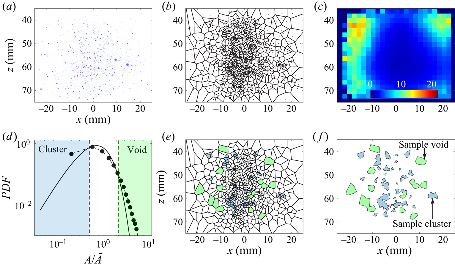
Figure 5. (a) Representative raw Mie scattering image corresponding to the no co-flow test condition. (b) Centres of the droplets in panel (a) and the Voronoï cells. (c) Spatial variation of the locally averaged Voronoï cells area. (d) PDF of the Voronoï cells areas normalized by their local mean. Overlaid in panel (d) is the PDF  $_{\rm RPP}$ from (3.1). The dashed lines in panel (d) are $A/\bar {A} = 0.5$ and 2.2. (e) Cells with areas related to clusters (blue cells) and voids (green cells). (f) Clusters and voids corresponding to the Mie scattering image in panel (a).
Provided the droplets spatial distribution followed the RPP, the PDF of  $A/\bar {A}$, referred to as PDF $_\mathrm {RPP}$, could be estimated using that of Ferenc & Néda (Reference Ferenc and Néda2007) which is given by
 \begin{equation} {PDF}_{\rm RPP}=\frac{b^a}{\varGamma(a)}\left(A/\bar{A}\right)^{a-1}\exp^{({-}b A/\bar{A})}. \end{equation}
In (3.1),  $a$ and $b$ are fitting parameters with $a=b=3.5$, and $\varGamma$ is the gamma function with $\varGamma (a) = 3.32$. The variation of PDF $_{\rm RPP}$ versus $A/\bar {A}$ was obtained and presented by the black solid curve in figure 5(c). Additionally, using MATLAB, 800 images were synthetically generated by distributing particles inside the domain of investigation randomly, with the number of droplets identical to that shown in figure 5(a), and the PDF of $A/\bar {A}$ was calculated. It was confirmed that the PDF of the Voronoï cells normalized area for randomly distributed particles closely follows the right-hand side of (3.1). Next, the intersections of PDF $_{\rm RPP}$ and the PDF $(A/\bar {A})$ for the results in figure 5(d) were obtained, which are shown by the dashed lines corresponding to $A/\bar {A} = 0.5$ and 2.2. The Voronoï cells with area smaller than $0.5 \bar {A}$ were labelled as clusters, and Voronoï cells with area larger than $2.2\bar {A}$ were labelled as voids. The identified clusters and voids corresponding to the Mie scattering image in figure 5(a) are shown by the blue and green colour cells in figure 5(e). As can be seen, clusters or voids may feature connected boundaries forming larger clusters and voids. Following Andrade et al. (Reference Andrade, Hardalupas and Charalampous2022), in the present study, the graph theory was used to identify and group the clusters/voids cells that are interconnected. For the results presented in figure 5(e), the identified clusters and voids are shown in figure 5(f). These clusters and voids were used for further analysis in § 4. It is important to note that the identified clusters and voids are formed due to both the interaction of the droplets with the background turbulent flow as well as (potentially) the air entrainment into the spray. Isolating the effect of the latter from that of the former on the clustering is not possible and was not performed in the present study.
3.2. Droplets location and diameter estimation
The ILIDS images were reduced to estimate the droplets location and diameters. A summary of the processes followed to reduce the ILIDS images is illustrated in figure 6. For clarity purposes, a cropped view of a representative raw ILIDS image is shown in figure 6(a), which corresponds to the test condition with two perforated plates and the mean bulk flow velocity of 14.0 m s $^{-1}$. Following the procedure used by Bocanegra Evans et al. (Reference Bocanegra Evans, Dam, van der Voort, Bertens and van de Water2015), the image shown in figure 6(a) was convoluted with a disk-shaped mask and the resultant image is shown in figure 6(b). The convoluted image features local maxima, which correspond to the centres of the droplets. The locations of the droplets centres were obtained, with the corresponding results shown by the black circular data points in figure 6(c). The variations of the light intensity along the lines that pass through the droplets centres and are normal to the corresponding fringe pattern were considered, with a sample fringe pattern and light intensity variation for one droplet shown in figure 6(d,e), respectively. Then, the fast Fourier transform of the light intensity variation corresponding to each droplet was obtained and the number of fringes was calculated. Finally, the droplet diameter was calculated using the number of fringe patterns and (2.1). Figure 6(f) presents the centres of the droplets as well as the blue circles, with their diameter relating to the droplets’ diameter. The diameters of the blue circles scale with the diameter of the red circle shown in the figure.

Figure 6. (a) Cropped view of a representative raw ILIDS image corresponding to the test condition with two perforated plates and mean bulk flow velocity of 14.0 m s $^{-1}$. (b) Convolution of the results in panel (a) using a disk-shaped mask. (c) Identified droplets centres. (d) Inset of panel (a), highlighting a sample fringe pattern. (e) Variation of the light intensity normal to the fringe pattern in panel (d). (f) Droplets centres and their corresponding diameters.
4. Results
The results are grouped into four subsections. In the first subsection, the characteristics of the background turbulent flow and the droplets diameter are discussed. In the second subsection, the degree of clustering is investigated. In the third subsection, the geometrical characteristics of the clusters and voids are presented. Finally, the joint characteristics of the clusters/voids and the droplets are presented in the last subsection.
4.1. Background flow and droplet diameter characteristics
The variations of the axial velocity mean ( $\bar {u}$) and RMS fluctuations ( $u^\prime$) along the $x$-axis are presented in the first and second rows of figure 7, respectively. The results in the first to fourth columns correspond to the mean bulk flow velocities of 3.5, 7.0, 10.5 and 14.0 m s $^{-1}$, and are shown using circular-, square-, triangular- and diamond-shaped data symbols, respectively. The blue, green and red colours pertain to zero, one and two perforated plates, respectively. The results presented in figure 7(a–d) feature a mean velocity deficit near $x=0$, which is due to the wake of the spray injector, similar to the results presented by Petry et al. (Reference Petry, Schäfer, Lammel and Hampp2022). Also, the mean velocity profiles are nearly symmetric for the test conditions without a perforated plate; however, these profiles are nearly asymmetric for test conditions with one and two perforated plates, which are similar to those reported by Kheirkhah & Gülder (Reference Kheirkhah and Gülder2015). Such asymmetry of the mean velocity profile is speculated to be caused by the relative positioning of the perforated plate with respect to the plane of the velocity measurements.

Figure 7. (a–d) Mean streamwise velocity for the mean bulk flow velocities of 3.5, 7.0, 10.5 and 14.0 m s $^{-1}$, respectively. (e–h) RMS streamwise velocity fluctuations for the mean bulk flow velocities of 3.5, 7.0, 10.5 and 14.0 m s $^{-1}$, respectively.
The results in figure 7(e–h) shows that for all tested mean bulk flow velocities and for the majority of the horizontal locations, the RMS of the streamwise velocity for one perforated plate is smaller than that for two perforated plates, which agrees with the results of past investigations, see for example those of Kheirkhah & Gülder (Reference Kheirkhah and Gülder2015). The results in figure 7(e–h) also show that the values of  $u^\prime$ for no perforated plate are larger than those of one perforated plate and close to those of two perforated plates. It is speculated that the reason for the values of $u^\prime$ for no perforated plate being relatively large is due to the turbulence generated by the supporting bars of the tube holder shown in figure 2(a) and the wake of the spray injector. To assess this speculation, HWA experiments for a free jet (without the spray injector and without the tube holder) were performed (not presented as a test condition in table 1) and the values of $u^\prime$ were obtained. These were significantly smaller than those for the first turbulence generation mechanism. For example, for $U=7.0$ m s $^{-1}$ and at $x =0$, $u^\prime =0.34$ m s $^{-1}$ for a free jet without the spray injector and the tube holder; however, this parameter is 1.07 m s $^{-1}$ with the injector and tube holder installed (i.e. the first turbulence generation mechanism). We speculate the reason for the values of $u^\prime$ being relatively smaller for the second turbulence generation mechanism (i.e. one perforated plate) than those for the first turbulence generation mechanism (zero perforated plate) is the break up of the eddies generated in the wake of the tube-holder bars by the perforated plate. The decrease of the RMS velocity fluctuations by the addition of the perforated plates has been reported by, for example, Wang et al. (Reference Wang, Yu, Zhang, Zhang and Huang2019).
The PDF of the droplet diameter for the first, second and third turbulence generation mechanisms are presented in figure 8(a–c), respectively. The PDFs were obtained considering all droplets within the field of view of the ILIDS measurements. For comparison purposes, the PDF of the droplet diameter for the no co-flow test condition is overlaid on figure 8(a–c) using the black circular data symbol. For the probability density function calculations, an 11.5  $\mathrm {\mu }$m droplet diameter bin size was used, since this led to the best presentation of the results. For all test conditions, the mean ( $\bar {d}$) and most probable droplet diameters were obtained and presented in figure 9(a,b), respectively. In figure 9(a,b), the error bars present twice the RMS of the droplet diameter fluctuations and the PDF bin size, respectively. The results in figure 9(b) show that the maximum change in the most probable droplet diameter as a result of changing the test condition is approximately $34-28=6\,\mathrm {\mu }\mathrm {m}$. This is smaller than the bin size (11.5 $\mathrm {\mu }$m) used for the PDF of the droplet diameter calculation. Thus, the results in figure 9(b) suggest that the most probable diameter of the droplets does not change noticeably by increasing the mean bulk flow velocity or changing the turbulence generation mechanism. This is speculated to be due to the measurement field of view being close to the injector, which strongly impacts the droplet diameter PDF. This finding is similar to that reported by Wang, Dalla Barba & Picano (Reference Wang, Dalla Barba and Picano2021). In fact, the study of Wang et al. (Reference Wang, Dalla Barba and Picano2021) showed that at relatively small vertical distances from the injector (less than 5 diameter of the nozzle) and for bulk flow Reynolds numbers comparable to those of the present study, changing this parameter does not influence the mean droplet diameter. The lack of sensitivity of the droplet diameter PDF to the test conditions, see figure 8, may have implications for the calculation of the Stokes number discussed earlier. Although the most probable droplet diameter is used for the estimation of the Stokes number, the PDFs of the droplet diameter do not change by changing the test condition. That is, alternative definitions of the Stokes number will yield similar trends in the present study, as a representative size for the droplet diameter will not change by varying the test conditions. Although the droplets diameter PDF estimated in the entire domain of investigation is not sensitive to the tested mean bulk flow velocity and the utilized turbulence generation mechanism, it is yet to be investigated how/if these parameters influence the PDF of the droplet diameter within the clusters and voids, which are studied in the following subsections.

Figure 8. (a–c) PDFs of the droplet diameter for no perforated plate, one perforated plate and two perforated plates, respectively. The black circular data points are the PDF of the no co-flow test condition, which is repeated in panels (a–c) for comparison purposes.

Figure 9. (a,b) Variations of the mean and most probable droplet diameter versus the mean bulk flow velocity for all test conditions.
4.2. The droplets degree of clustering
The Voronoï cells were used to study the droplets degree of clustering, following the procedure discussed in § 3. For all test conditions, the PDFs of the Voronoï cells area ( $A$) are calculated and presented in figure 10(a). Also, the PDFs of the Voronoï cells area normalized by the locally averaged area ( $A/\bar {A}$) are shown in figure 10(b) for all test conditions. As can be seen, the PDFs of $A/\bar {A}$ collapse for all test conditions, which is similar to the results presented by Obligado et al. (Reference Obligado, Teitelbaum, Cartellier, Mininni and Bourgoin2014) and Monchaux et al. (Reference Monchaux, Bourgoin and Cartellier2010). Overlaid on figure 10 is the PDF of the normalized area of the Voronoï cells provided these cells are spatially distributed following the RPP, with the formulation of PDF $_{\rm RPP}$ presented in (3.1). The results in figure 10 show that, for all test conditions, the PDFs of $A/\bar {A}$ intersect with PDF $_{\rm RPP}$ at $A/\bar {A} = 0.5$ and 2.2, which are shown by the vertical dashed lines in figure 10(b) and are similar to those shown in figure 5(c). Using the above normalized areas and following the procedure presented in § 3.1, the clusters and voids were identified, and the degree of clustering is studied below.

Figure 10. (a) PDFs of the Voronoï cells area, PDF  $(A)$, for all test conditions. (b) PDF of the Voronoï cells area normalized by the locally averaged area. The solid black curve in panel (b) is the PDF of the normalized Voronoï cells area provided they were distributed following an RPP, with the formulation given in (3.1). The dashed lines in panel (b) correspond to $A/\bar {A} = 0.5$ and 2.2.
The degree of clustering,  $(\sigma -\sigma _{{\rm RPP}})/\sigma _{{\rm RPP}}$, is presented in figure 11(a) for all test conditions. The results in the figure show that for test conditions with the co-flow, the degree of clustering is generally larger than that for the no co-flow test condition. Since the background turbulent flow characteristics do not necessarily vary monotonically with the number of perforated plates, best comparisons are obtained when the degree of clustering is presented versus $St$ and $Re_\lambda$. The variations of the degree of clustering versus the Stokes number and the Taylor-length-scale-based Reynolds number are presented in figure 11(b,c), respectively. In addition to the results of the present study, those of Obligado et al. (Reference Obligado, Teitelbaum, Cartellier, Mininni and Bourgoin2014), Monchaux et al. (Reference Monchaux, Bourgoin and Cartellier2010), Sumbekova et al. (Reference Sumbekova, Cartellier, Aliseda and Bourgoin2017) and Petersen, Baker & Coletti (Reference Petersen, Baker and Coletti2019) are also overlaid on these figures. Analysis of the results presented by Monchaux et al. (Reference Monchaux, Bourgoin and Cartellier2010) suggests that, for relatively small values of the Stokes number ( $St \lesssim 10$) and for relatively small values of the Taylor-length-scale-based Reynolds number ( $Re_\lambda \lesssim 200$), as $St$ increases, the degree of clustering initially increases and reaches a maximum. Further increasing the Stokes number decreases the degree of clustering. For relatively small values of the Stokes number but relatively large values of the Taylor-length-scale-based Reynolds number ( $Re_\lambda \gtrsim 200$), the degree of clustering is primarily influenced by $Re_\lambda$, see the results of Sumbekova et al. (Reference Sumbekova, Cartellier, Aliseda and Bourgoin2017). Specifically, increasing $Re_\lambda$ increases the degree of clustering. Compared to past investigations, which correspond to particle-laden flows with relatively small Stokes numbers, for relatively large values of this parameter ( $St \gtrsim 10$) and small values of the Taylor-length-scale-based Reynolds number, the degree of clustering is relatively small; and increasing $St$ slightly increases the degree of clustering, plateauing at approximately 0.3. Acknowledging that the background turbulent flow of the present study may not be isotropic, which is different from the studies of Obligado et al. (Reference Obligado, Teitelbaum, Cartellier, Mininni and Bourgoin2014), Monchaux et al. (Reference Monchaux, Bourgoin and Cartellier2010), Sumbekova et al. (Reference Sumbekova, Cartellier, Aliseda and Bourgoin2017) and Petersen et al. (Reference Petersen, Baker and Coletti2019), further investigations are required to consider the influence of anisotropy of the background flow on the degree of clustering.

Figure 11. (a–c) Degree of clustering versus the mean bulk flow velocity, the Stokes number and Taylor-length-scale-based Reynolds number, respectively. Overlaid on panel (b,c) are the results of Obligado et al. (Reference Obligado, Teitelbaum, Cartellier, Mininni and Bourgoin2014), Monchaux et al. (Reference Monchaux, Bourgoin and Cartellier2010), Sumbekova et al. (Reference Sumbekova, Cartellier, Aliseda and Bourgoin2017) and Petersen et al. (Reference Petersen, Baker and Coletti2019).
Wang et al. (Reference Wang, Wan, Yang, Wang and Chen2020) performed three-dimensional (3-D) direct numerical simulation (DNS) of particles clustering in homogeneous and isotropic turbulent flow in a box for Stokes numbers ranging from approximately 0 to 7. They estimated the standard deviation of the 3-D Voronoï cells volume. Results of Wang et al. (Reference Wang, Wan, Yang, Wang and Chen2020) show that the standard deviation of the 3-D Voronoï cells volume increases by increasing the Stokes number from approximately 0 to 1. However, further increase of the Stokes number to approximately 7 plateaus the standard deviation of the Voronoï cells volume. Although the analysis of Wang et al. (Reference Wang, Wan, Yang, Wang and Chen2020) is performed for the RMS of the Voronoï cells volume (which is different than the degree of clustering that pertains to the Voronoï cells area), the reported trend of Wang et al. (Reference Wang, Wan, Yang, Wang and Chen2020) follows that presented in figure 11(b) for matching Stokes numbers. Nevertheless, to our best knowledge, the plateau of the degree of clustering with increasing the Stokes number for  $St \gtrsim 7$ is reported in the present study for the first time.
4.3. The geometrical characteristics of clusters and voids
Clustering of the clusters, length scales of the clusters and voids as well as how these are influenced by the non-dimensional parameters are discussed in the following subsections.
4.3.1. Clustering of the clusters
Although the analysis presented in § 4.2 allows for understanding the droplets degree of clustering, it does not provide insight into the clustering of the clusters, which is discussed in this subsection.
A representative spatial distribution of the clusters for the no co-flow test condition is presented in figure 12(a), see the blue regions in the figure. The centres of the area of the clusters were obtained and are shown by the black circular symbols in figure 12(a,b). The Voronoï cells associated with the centre of areas of the clusters were obtained and are shown in figure 12(b) using the blue lines. For all test conditions, the PDF of the Voronoï cells area obtained using the centre area of the clusters ( $\tilde {A}$) divided by its mean value ( $\overline {\tilde {A}}$) is presented in figure 13. Also overlaid on the figure is the PDF $_{\rm RPP}$. Analysis similar to that performed for calculating the degree of clustering was employed to estimate the standard deviation of the area of the Voronoï cells formed by the clusters centre of area normalized by their mean value. This was performed to asses the probability of the clustering of the clusters. For all test conditions, the standard deviation of $\tilde {A}/\overline {\tilde {A}}$ was calculated and it ranges from 0.3 to 0.4, which is smaller than $\sigma _{{\rm RPP}}=0.53$. Monchaux et al. (Reference Monchaux, Bourgoin and Cartellier2010) discussed that the standard deviations smaller than that of the RPP suggest that the clusters are distributed in an organized manner. As a result, the clustering of the clusters does not occur in the present study. Similar to the above analysis, Obligado, Cartellier & Bourgoin (Reference Obligado, Cartellier and Bourgoin2015) also investigated the clustering of the clusters. Their results show that the degree of clustering of the clusters was 0.8. Using the definition of the degree of clustering, the above means that the standard deviation of the area of the Voronoï cells formed by the clusters centre of area normalized by their mean value is $0.53\times (0.8+1) \approx 1$ for the results of Obligado et al. (Reference Obligado, Cartellier and Bourgoin2015), which is significantly larger than those of the present study.

Figure 12. (a) Representative clusters. (b) The Voronoï cells formed by the clusters centre of area. In panel (a,b), the clusters centres of area are shown by the solid black data symbol. The results in panel (a,b) correspond to the no co-flow test condition.

Figure 13. PDFs of the normalized Voronoï cells area formed by the clusters centre of area. The black solid curve is the PDF  $_{\rm RPP}$.
4.3.2. Length scale of clusters and voids
Following Petersen et al. (Reference Petersen, Baker and Coletti2019), the cluster and void length scales were defined as  $L_{{\rm c}} = \sqrt {A_{{\rm c}}}$ and $L_{{\rm v}} = \sqrt {A_{{\rm v}}}$, respectively, with $A_{{\rm c}}$ and $A_{{\rm v}}$ being the cluster and void areas. The PDFs of $L_{{\rm c}}$ and $L_{{\rm v}}$ are presented in figures 14 and 15, respectively. The results in figures 14(a–d) and 15(a–d) correspond to mean bulk flow velocities of 3.5, 7.0, 10.5 and 14.0 m s $^{-1}$, respectively. For comparison purposes, the PDFs of the cluster and void length scales corresponding to the no co-flow test condition is presented by the solid black circular data symbol on the figures. The results in figures 14 and 15 show that for both clusters and voids, the presence of the co-flow generally leads to larger values of the most probable length scales.

Figure 14. (a–d) PDFs of the cluster length scale for mean bulk flow velocities of  $U=3.5$, 7.0, 10.5 and 14.0 m s $^{-1}$, respectively. Overlaid by the black circular data symbol in panel (a–d) is the PDF of the cluster length scale for the no co-flow test condition.

Figure 15. (a–d) PDFs of the void length scale for the mean bulk flow velocities of 3.5, 7.0, 10.5 and 14.0 m s $^{-1}$, respectively. The black circular data symbol is the PDF of the void length scale for the no co-flow test condition.
Although the most probable cluster and void length scales are of importance, the majority of past investigations studied the relations between the mean values of the above length scales and the non-dimensional parameters, such as Taylor-length-scale-based Reynolds and Stokes numbers. The mean cluster and void length scales versus the mean bulk flow velocity are presented in figure 16(a,b), respectively. The error bars in the figures are twice the standard deviation of the corresponding data. For comparison purposes, the Taylor and integral length scales are also presented in figure 16(c,d), respectively. As can be seen, increasing the mean bulk flow velocity increases both the mean cluster and void length scales. The results show that cluster size is larger than the Taylor length scale but smaller than the integral length scale. The mean void length scale is, however, close to the integral length scale.

Figure 16. (a,b) Mean cluster and void length scales versus the mean bulk flow velocity, respectively. (c,d) Taylor and integral length scales versus the mean bulk flow velocity, respectively.
Variations of  $\overline {L_{{\rm c}}}$ normalized by the Kolmogorov length scale versus $Re_\lambda$ is presented in figure 17(a). Also, overlaid on the figure are the results of Obligado et al. (Reference Obligado, Teitelbaum, Cartellier, Mininni and Bourgoin2014) and Sumbekova et al. (Reference Sumbekova, Cartellier, Aliseda and Bourgoin2017), which are highlighted by the black dashed ellipse in the figure and correspond to relatively small Stokes numbers ( $0 \lesssim St \lesssim 10$). The results of the present study are highlighted by the dashed red rectangle. As can be seen, the normalized cluster length scale of the present study and those of Obligado et al. (Reference Obligado, Teitelbaum, Cartellier, Mininni and Bourgoin2014) and Sumbekova et al. (Reference Sumbekova, Cartellier, Aliseda and Bourgoin2017) do not follow a trend. Thus, variation of $\overline {L_{{\rm c}}}/\eta$ versus the Stokes number were obtained and presented in figure 17(b). The results of Obligado et al. (Reference Obligado, Teitelbaum, Cartellier, Mininni and Bourgoin2014) and Sumbekova et al. (Reference Sumbekova, Cartellier, Aliseda and Bourgoin2017) as well as Petersen et al. (Reference Petersen, Baker and Coletti2019) are overlaid on the figure for comparison. As can be seen, the normalized mean cluster length scale follows a trend when presented against the Stokes number. Specifically, it can be seen that increasing $St$ almost linearly increases $\overline {L_{{\rm c}}}/\eta$. Increasing the Stokes number to relatively large values leads to the response time of the droplets to become close to the time scale of large eddies. Thus, at large Stokes numbers, the droplets form relatively large clusters. This is consistent with the results presented by Petersen et al. (Reference Petersen, Baker and Coletti2019).

Figure 17. (a,b) Mean cluster length scale normalized by the Kolmogorov length scale versus  $Re_\lambda$ and $St$, respectively. Overlaid on panel (a,b) are the results of Obligado et al. (Reference Obligado, Teitelbaum, Cartellier, Mininni and Bourgoin2014), Sumbekova et al. (Reference Sumbekova, Cartellier, Aliseda and Bourgoin2017) and Petersen et al. (Reference Petersen, Baker and Coletti2019). (c,d) Mean void length scale normalized by the integral length scale versus $Re_\lambda$ and $St$, respectively.
Variations of  $\overline {L_{{\rm v}}}/\varLambda$ versus $Re_\lambda$ and $St$ are presented in figure 17(c,d), respectively. Compared to the mean cluster length scale that can become approximately 100 times larger than the Kolmogorov length scale, the results in figure 17(c,d) show that the mean void length scale is of the order of the integral length scale. For large Stokes numbers, the droplets feature relatively large inertia, they interact with large scale eddies and, as a result, the droplets position at the periphery of the large scale eddies. This would suggest that for large Stokes numbers (such as those of the present study), the regions inside the large eddies correspond to voids; and, as a result, these regions size is approximately the voids length scale, as shown in figure 17(d). Yoshimoto & Goto (Reference Yoshimoto and Goto2007) performed DNS of particles interacting with homogeneous and isotropic turbulence in a box, and they indeed showed that for $St = 10$, the length scale of voids saturate at the integral length scale of the turbulent flow. The results of the present study extends the findings of Yoshimoto & Goto (Reference Yoshimoto and Goto2007) from homogeneous and isotropic turbulence in a box to sprays in a turbulent co-flow with Stokes numbers up to 25.
4.4. The inter-cluster and inter-void characteristics
The results discussed in §§ 4.1–4.3 allow for understanding the characteristics of the droplets as well as those of clusters and voids individually; however, our understanding related to joint characteristics of the droplets and clusters/voids remains to be developed. In the following, the number density of the droplets inside the clusters and voids as well as the joint probability density function (JPDF) of the droplets diameter and clusters/voids areas are investigated.
4.4.1. Number densities of droplets inside clusters and voids
Figure 18 presents the JPDF of the number of droplets ( $N_{{\rm P}}$) inside the clusters and the area of the clusters. The contours are presented on a logarithmic scale (with a base of 10) for improving the clarity of presentation. The JPDFs in figure 18(a,f,k) correspond to the no co-flow test condition, are repeated and are presented for comparison purposes. The results in the second to fifth columns pertain to the mean bulk flow velocities of 3.5, 7.0, 10.5, and 14.0 m s $^{-1}$, respectively. The results in (b–e), (g–j) and (l–o) correspond to zero, one and two perforated plates, respectively. As can be seen, there exists a positive correlation between the number of particles and the area of the clusters, i.e. larger clusters contain more droplets. It can also be seen that increasing the mean bulk flow velocity decreases the slope of the relation between $N_{{\rm P}}$ and $A_{{\rm c}}$, suggesting that the clusters dilute with increasing $U$. To quantify this, the combination of ( $N_{{\rm P}},A_{{\rm c}}$) data points at which the JPDF significantly changes by changing $A_{{\rm c}}$ at a fixed $N_{{\rm P}}$ were obtained, with representative results shown by the white circular data symbols in figure 18(a). The linear fits to these white data points were obtained, and the slopes of the lines were referred to as $m_1$ and $m_2$. Variations of $m_1$, $m_2$ and their average, $\bar {m} = 0.5(m_1+m_2)$, versus the mean bulk flow velocity are shown in figure 19(a–c), respectively. These parameters quantify the number density of the droplets within the clusters. Similar to the above analysis, the JPDF of the number of droplets inside the voids and the area of the voids were obtained, with the corresponding results presented in figure 20. The figure indicators in figure 20 are identical to those in figure 18. Similar to the analysis presented for the results in figure 18(a–c), the slopes ( $m^\prime _1$, $m^\prime _2$ and $\overline {m^\prime } = 0.5(m^\prime _1+m^\prime _2)$) for the results in figure 20 were extracted and are shown in figure 19(d–f). Comparison of the results presented in figure 19(a–c) with those in figure 19(d–f) suggests that the number density of droplets within the clusters is generally one order of magnitude larger than that in the voids.

Figure 18. Logarithmic JPDF of the number of droplets within a given cluster area. Panel (a,f,k) corresponds to the no co-flow test condition and is repeated in each row for comparison purposes. The second to fifth columns correspond to the mean bulk flow velocities of 3.5, 7.0, 10.5 and 14.0 m s $^{-1}$, respectively. (b–e), (g–j) and (l–o) First to third turbulence generation mechanisms, respectively.

Figure 19. (a–c) Variations of  $m_1$, $m_2$ and $0.5(m_1+m_2)$ versus $U$, respectively. (d–f) Variations of $m^\prime _1$, $m^\prime _2$ and $0.5(m^\prime _1+m^\prime _2)$ versus $U$, respectively.

Figure 20. Logarithmic JPDF of the number of droplets and void area. Panel (a,f,k) corresponds to the no co-flow test condition and is repeated in each row for comparison purposes. The second to fifth columns correspond to the mean bulk flow velocities of 3.5, 7.0, 10.5 and 14.0 m s $^{-1}$, respectively. (b–e), (g–j) and (l–o) First to third turbulence generation mechanisms, respectively.
To investigate the effect of the non-dimensional parameters on the above number densities, the variations of  $\bar {m}$ versus the Taylor-length-scale-based Reynolds and Stokes numbers are presented in figure 21(a,b), respectively. Also overlaid on the figures are the error bars, whose lengths correspond to $m_2-m_1$. Similarly, the variations of $\overline {m^\prime }$ versus the Taylor-length-scale-based Reynolds and Stokes numbers are also shown in figure 21(c,d), respectively, with the lengths of the error bars being $m^\prime _2-m^\prime _1$. The results suggest that for $St \gtrsim 10$, the number densities of the droplets inside the clusters and voids are nearly independent of the Stokes and the Taylor-length-scale-based Reynolds numbers and equal 0.45 and $0.06\,\mathrm {mm}^{-2}$, respectively. However, for $St \lesssim 10$, increasing the Taylor-length-scale-based Reynolds number (which is accompanied by increase of the Stokes number) nearly decreases the number densities of the droplets in the clusters and voids.

Figure 21. (a,b) Variations of  $\bar {m}$ versus $Re_\lambda$ and $St$, respectively. (c,d) Variations of $\overline {m^\prime }$ versus $Re_\lambda$ and $St$, respectively.
On one hand, the results presented in figure 4 showed that increasing the Taylor-length-scale-based Reynolds and Stokes numbers both decrease the spray volume fraction. On the other hand, for  $St \lesssim 10$, the results in figure 21 showed that increasing both $Re_\lambda$ and $St$ also decrease $\bar {m}$ and $\overline {m^\prime }$. It is of interest to investigate the contributions of the decay of the number densities of the droplets inside the clusters and voids to the potential decay in the total number density of the droplets and if these contributions change by changing $Re_\lambda$ and $St$. Figures 22(a) and 22(b) present the ratio of the total number of droplets detected in the Mie scattering field of view divided by the area of the field of view, $M$, versus the Taylor-length-scale-based Reynolds and Stokes numbers, respectively. As can be seen, increasing these non-dimensional parameters decreases $M$, which is anticipated considering the decreasing trend in figure 4(c) and that the most probable droplet diameter is nearly unchanged by changing the test conditions. The variations of $\bar {m}/M$ versus $Re_\lambda$ and $St$ are presented in figure 22(c,d). Similarly, the variations of $\overline {m^\prime }/M$ versus $Re_\lambda$ and $St$ are presented in figure 22(e,f), respectively. In figures 22(c,d) and 22(e,f), the lengths of the error bars are $m_2-m_1$ and $m_2^\prime -m_1^\prime$ normalized by the total droplets number density of the corresponding test condition. The results show that the number density of the droplets within the clusters and voids are 5.5 and 0.8 times the total number density, see the dashed lines in the figures, and these ratios do not change by changing the test conditions.

Figure 22. (a,b) Variations of the total number density versus  $Re_\lambda$ and $St$, respectively. (c,d) Variations of the number density of the droplets in the clusters divided by the total number density versus $Re_\lambda$ and $St$, respectively. (e,f) Variations of the number density of droplets in the voids divided by the total number density versus $Re_\lambda$ and $St$, respectively.
4.4.2. Joint probability density function of droplet diameter and cluster/void area
The JPDF of the clusters normalized area ( $A_{{\rm c}}/\overline {A_{{\rm c}}}$) and the mean diameter ( $\tilde {d}$) of the droplets within the clusters with normalized area of $A_{{\rm c}}/\overline {A_{{\rm c}}}$ is presented in figure 23. The bin size for the droplet diameter in the clusters was selected following the discussions presented in Appendix C. For presentation purposes, the JPDF contours are shown on a logarithmic scale with the base of 10. The results presented in figure 23(a,f,k) pertain to the no co-flow test condition, are identical and are shown for comparison purposes. The contours presented in the second to fifth columns correspond to the mean bulk flow velocities of 3.5, 7.0, 10.5 and 14.0 m s $^{-1}$, respectively. The results in figures 23(b–e), 23(g–j) and 23(l–o) pertain to test conditions with zero, one and two perforated plates, respectively. As can be seen, for all test conditions, the clusters with relatively small areas ( $A_{{\rm c}}/\overline {A_{{\rm c}}} \lesssim 1$) are highly likely to exist. This is due to the PDF of the cluster length scale being skewed towards small values, as shown in figure 14. It can also be seen that near $\tilde {d} \approx 30\,\mathrm {\mu }$m, which is close to the most probable droplet diameter measured in the ILIDS field of view and tabulated in table 1, the JPDFs feature significant values for a large range of cluster sizes. This means that for all test conditions, the majority of the clusters carry the droplets with the most probable diameter.

Figure 23. Logarithmic JPDF of the normalized clusters area ( $A_{{\rm c}}/\overline {A_{{\rm c}}}$) and the mean diameter ( $\tilde {d}$) of the droplets that exist within the cluster with normalized area of $A_{{\rm c}}/\overline {A_{{\rm c}}}$. Panel (a,f,k) corresponds to the no co-flow test condition and is repeated in each row for comparison purposes. The second to fifth columns correspond to the mean bulk flow velocities of 3.5, 7.0, 10.5 and 14.0 m s $^{-1}$, respectively. Panels (b–e), (g–j) and (l–o) present the results for the first to third turbulence generation mechanisms, respectively.
Comparison of the JPDFs for the no co-flow test condition (see panel a,f,k) with those that the co-flow provided shows that the probability of finding large droplets (mean diameter larger than approximately 100  $\mathrm {\mu }$m) within a given normalized cluster area increases by adding the co-flow. This means that the presence of the co-flow facilitates the clustering of the large droplets. To quantify the effect of the co-flow on $\tilde {d}$, the contour of JPDF $(A_{{\rm c}}/\overline {A_{{\rm c}}}) = 10^{-3.5}$ was considered. Then, the intersections of this contour with a given normalized cluster area (here, $A_{{\rm c}}/\overline {A_{{\rm c}}}=1$) were obtained, which are referred to as $\widetilde {d_1}$ and $\widetilde {d_2}$, see figure 23(b). The values of $\widetilde {d_1}$ and $\widetilde {d_2}$ change by varying the values of the selected JPDF as well as the selected $A_{{\rm c}}/\overline {A_{{\rm c}}}$; however, the trends of variation for $\widetilde {d_2}-\widetilde {d_1}$ with the governing parameters are independent of the selected JPDF value and $A_{{\rm c}}/\overline {A_{{\rm c}}}$. For all test conditions with the co-flow, the variations of $\widetilde {d_2}-\widetilde {d_1}$ versus $Re_\lambda$ and $St$ were obtained and presented in figure 24(a,b), respectively. The results show that increasing $Re_\lambda$ and $St$ generally increases $\widetilde {d_2}-\widetilde {d_1}$. As shown in figure 16(d) and as tabulated in table 1, increasing the mean bulk flow velocity increases the integral length scale and decreases the Kolmogorov length scale. Thus, adding the co-flow (which is equivalent to increasing the $Re_\lambda$) increases the range of the turbulent eddy sizes. Following the mechanisms proposed by, for example, Goto & Vassilicos (Reference Goto and Vassilicos2006), since turbulent eddies are responsible for the clustering of the droplets, the larger range of turbulent eddy sizes (see figure 16c,d) could increase the possibility of a broader range of droplet diameters to be positioned inside the clusters. As a result, a positive relation between $\widetilde {d_2}-\widetilde {d_1}$ and $Re_\lambda$ as well as $St$ is observed. This also suggests that the mechanism proposed by, for example, Goto & Vassilicos (Reference Goto and Vassilicos2006) for droplets clustering may be extended to relatively large Stokes numbers of approximately 25, which was examined in the present study.

Figure 24. (a,b) Variations of  $\widetilde {d_2}-\widetilde {d_1}$ versus the Taylor-length-scale-based Reynolds and Stokes numbers, respectively.
An analysis similar to the above was performed to investigate the joint characteristic of droplets and voids. Figure 25 presents the JPDF of the voids normalized area ( $A_{{\rm v}}/\overline {A_{{\rm v}}}$) versus the mean diameter of droplets within the voids ( $\widetilde {d^\prime }$). The bin size for the droplet diameter in the voids was selected following the discussions in Appendix C. Similar to figure 23, the first to fifth columns correspond to the no co-flow, $U = 3.5$, 7.0, 10.5 and 14.0 m s $^{-1}$ test conditions, respectively. Also, the results in the first to third rows pertain to the first to third turbulence generation mechanisms, respectively. The results presented in figure 25 show that the presence of the co-flow (compared with the no co-flow test condition) increases the probability of relatively large droplets to reside within the voids. The results in the second to fifth columns of figure 25 suggest that increasing the mean bulk flow velocity and changing the turbulence generation mechanisms do not substantially change JPDF $(A_{{\rm v}}/\overline {A_{{\rm v}}},\widetilde {d^\prime })$. This suggests that the turbulent co-flow may not facilitate positioning of the droplets within the voids.

Figure 25. Logarithmic JPDF of the normalized area of the voids ( $A_{{\rm v}}/\overline {A_{{\rm v}}}$) and the mean diameter of the droplets that exist within the voids ( $\widetilde {d^\prime }$). Panel (a,f,k) corresponds to the no co-flow test condition and is repeated in each row for comparison purposes. The second to fifth columns correspond to the mean bulk flow velocities of 3.5, 7.0, 10.5 and 14.0 m s $^{-1}$, respectively. Panels (b–e), (g–j) and (l–o) present the results for the first to third turbulence generation mechanisms, respectively.
5. Concluding remarks
Separate and joint characteristics of droplets diameter and clusters/voids size at relatively large Stokes numbers were investigated experimentally. Simultaneous Mie scattering and interferometric laser imaging for droplet sizing (ILIDS) were performed to acquire the spatial distribution of the droplets and their corresponding diameters. Also, separate hotwire anemometry was performed to characterize the background turbulent flow. A flow apparatus was used to produce a water spray injected in a turbulent co-flow of air. Mean bulk flow velocities of 0 (no co-flow), 3.5, 7.0, 10.5 and 14.0 m s $^{-1}$ were examined. Three turbulence generation mechanisms (zero, one and two perforated plates) were used in the present study. The above mean bulk flow velocities and turbulence generation mechanisms allowed to vary the Kolmogorov-time-scale-based Stokes number and Taylor-length-scale-based Reynolds number from 3 to 25 as well as 10 to 38, which correspond to relatively large and small values (compared with those reported in the literature), respectively. The volume fraction of the spray was varied from approximately $10^{-6}$ to $2\times 10^{-6}$, which rendered the tested sprays as dilute.
The Voronoï analysis was performed to calculate the degree of clustering as well as to identify the clusters and voids. The results showed that the addition of the co-flow to the spray generally increases the degree of clustering compared with the no co-flow condition. The results of the present study and those of past investigations were compiled and it was obtained that for relatively small values of the Stokes number ( $St \lesssim 10$) and for relatively small values of the Taylor-length-scale-based Reynolds number ( $Re_\lambda \lesssim 200$), as $St$ increases, the degree of clustering initially increases and reaches a maxim value at $St\approx 2\unicode{x2013}4$. Further increasing the Stokes number decreases the degree of clustering. For relatively small values of the Stokes number but relatively large values of the Taylor-length-scale-based Reynolds number ( $Re_\lambda \gtrsim 200$), the degree of clustering appears to be primarily influenced by $Re_\lambda$. Specifically, increasing $Re_\lambda$ increases the degree of clustering. Compared with past investigations, which correspond to particle-laden flows with relatively small Stokes numbers, for relatively large values of this parameter ( $St \gtrsim 10$) and small values of the Taylor-length-scale-based Reynolds number, the degree of clustering is relatively small; and increasing $St$ slightly increases the degree of clustering, plateauing at approximately 0.3.
The clusters centre of area was obtained and the corresponding Voronoï cells were formed for all test conditions. The results showed that the standard deviation of these cells area normalized by their corresponding mean varies from 0.3 to 0.4 which is smaller than the standard deviation of a random Poisson process (i.e. 0.53). As a result, the clustering of the clusters does not occur for the conditions tested in the present study.
The length scales of the clusters and voids were estimated and compared with those of the background turbulent co-flow. The results showed that the mean void length scale was of the order of the integral length scale for all test conditions. However, the mean cluster length scale is smaller than the integral length scale but larger than the Taylor length scale. It was shown that increasing the Stokes number increases the mean cluster length scale to approximately 60 times the Kolmogorov length scale.
The results showed that the number density of the droplets within the clusters is approximately one order of magnitude larger than that for the voids, and both number densities decrease and then plateau with increasing the Stokes and Taylor-length-scale-based Reynolds numbers. It was obtained that the ratios of the clusters and voids number densities to the total number density of the spray are independent of the test conditions and nearly equal to 5.5 and 0.8, respectively. The joint probability density function analysis was used to study the joint characteristics of the droplets and clusters/voids. It was concluded that a relatively wide range of cluster length scales can accommodate the most probable droplet diameter (approximately 30  $\mathrm {\mu }$m) for all test conditions. It was shown that, although the joint PDF of the droplets diameter was not noticeably sensitive to the co-flow, increasing the Stokes and Taylor-length-scale-based Reynolds numbers increase the possibility of residing large droplets within the clusters. This was explained to be linked to increased range of eddy sizes interacting with droplets due to the increase of the above non-dimensional parameters. The present study provides insight into the number density of spray droplets within clusters and voids as well as the joint characteristics of the droplets and the cluster/voids area for relatively large Stokes numbers ( $St\gtrsim 10$). This study also illustrates how the above characteristics are influenced by the variation of the Stokes and Taylor-length-scale-based Reynolds numbers.
Acknowledgments
The authors are grateful for the financial support from the University of British Columbia through the Eminence Fund program. S. Kheirkhah acknowledges the financial support from the Canada Foundation for Innovation.
Declaration of interests
The authors report no conflict of interest.
Appendix A. Spray volume flow rate calibration
For the spray volume flow rate ( $\dot {Q}$) calibration, first, the spray injector shown in figure 2 was connected to a sealed container; then, the upstream pressure of the injector ( $P_{{\rm v}}$) was set to several values ranging from approximately 50 to 800 kPa using the pressure controller shown as item (2) in figure 1. For each set value of the upstream pressure, a high-precision scale was used to measure the collected water mass, which was converted to volume by using the water density at the laboratory temperature of 20 $^{\circ }$C. Then, the volume flow rate was calculated by dividing the volume of the collected water (in litres) to the time duration of the calibration experiment, which was 120 s. Figure 26 presents the variation of $\dot {Q}$ versus $P_{{\rm v}}$. For all conditions tested in the present study, $P_{{\rm v}}$ was set to 206 kPa, which led to a spray volume flow rate of 22 cubic centimetres per minute (see the black circular data symbol in figure 26).

Figure 26. Relation between the water vessel pressure and the spray flow rate.
Appendix B. Procedure for registering the Mie scattering images to the ILIDS images and correcting the centre discrepancy
The centres of the droplets identified from the ILIDS images are not identical to those obtained from the Mie scattering images, and a discrepancy exists between the centres of the droplets identified from the above diagnostics. In addition to the present study, such discrepancy is also noted and discussed in the past investigations, see for example those of Boddapati et al. (Reference Boddapati, Manish and Sahu2020) and Hardalupas et al. (Reference Hardalupas, Sahu, Taylor and Zarogoulidis2010). For the droplets and clusters/voids joint characteristics calculations, it is important to correct the discrepancy between the centres of the droplets obtained from the Mie scattering and ILIDS images. The procedure for correcting the above discrepancy and thus registering the Mie scattering to the ILIDS images is discussed in the following.
First, a 2-D target plate was manufactured and positioned in the location illuminated by the laser sheet in the experiments. Then, the images of the target plate were captured by the cameras used for collecting the Mie scattering and ILIDS images, with the collected images shown in figure 27(a,b), respectively. Eighteen points, see the green circles in figure 27(a), were considered and were identified in figure 27(b). The collective geometrical shape of these points was purposely selected to be asymmetric, facilitating the above identification. Then, the matrix that transforms data points in figure 27(a) to those in figure 27(b) was obtained. This transformation matrix was used for registering the Mie scattering images to the ILIDS images, with a representative result for such transformation discussed below.

Figure 27. (a,b) Images of the target plate captured by the Mie scattering and ILIDS cameras, respectively.
Representative and simultaneously acquired Mie scattering and ILIDS images are shown in figure 28(a,b), respectively. The results correspond to the test condition with one perforated plate and the mean bulk flow velocity of 10.5 m s $^{-1}$. Figure 28(c) presents the results in figure 28(a) after the application of the above transformation. Figure 28(d) shows that in figure 28(b) after application of the convolution discussed in § 3.2. The procedure discussed in § 3.2 was followed to identify the centres of the droplets from the results shown in figure 28(d), with the corresponding centres presented by the blue circular data points in figure 28(e). Overlaid on figure 28(e) are also the centres of the droplets obtained from binarizing the Mie scattering image in figure 28(c). The centres of the droplets obtained from the Mie scattering image are shown by the red cross data symbols in figure 28(e). As shown in this figure, a centre discrepancy exists even after the ILIDS image is registered to the Mie scattering image. The maximum centre discrepancy is approximately $59\,\mathrm {pixels}\times 0.0114\,\mathrm {mm}\,\mathrm {pixel}^{-1} \approx 0.7$ mm in our experiments, which is similar to that (approximately 1 mm) reported by Hardalupas et al. (Reference Hardalupas, Sahu, Taylor and Zarogoulidis2010). In the study by Hardalupas et al. (Reference Hardalupas, Sahu, Taylor and Zarogoulidis2010), the centre discrepancy is independent of the droplet diameter but varies linearly along the imaging plane. Such variation is used by Hardalupas et al. (Reference Hardalupas, Sahu, Taylor and Zarogoulidis2010) to correct the location of the droplets. In the present study, however, a different approach was used to that of Hardalupas et al. (Reference Hardalupas, Sahu, Taylor and Zarogoulidis2010) to address the centre discrepancy. Since the spray used in the present study was dilute, the maximum centre discrepancy was relatively small and that the simultaneously acquired Mie scattering images allowed for understanding the true location of the droplets centres, a sorting algorithm in MATLAB was used to relate the droplets in the ILIDS image to the corresponding Mie scattering image. This relation was used to correct the discrepancy in the droplets locations.

Figure 28. (a,b) Representative raw Mie scattering and ILIDS images, respectively. (c) Image obtained by mapping that shown in panel (a) to the imaging plane of the ILIDS camera. (d) Convolution of the results shown in panel (b) with a disk-shaped mask. (e) Centres of the droplets obtained from the ILIDS and Mie scattering images.
Appendix C. Statistical error in calculation of the mean droplet diameter within clusters and voids
The number of the droplets detected from the ILIDS images is not equal to that obtained from the Mie scattering images. This can lead to statistical error in the calculation of the mean droplet diameter within the clusters and voids. To estimate this error, the PDF of the number of droplets detected within a cluster using the ILIDS and Mie scattering techniques were obtained for all test conditions and are presented in figure 29(a,b), respectively. As can be seen, the most probable number of droplets detected within a cluster using the ILIDS ( $n^*_{{\rm ILIDS}}$) and Mie scattering ( $n^*_{{\rm Mie}}$) techniques are 3 and 11, respectively. It is acknowledged that the difference between $n^*_{{\rm ILIDS}}$ and $n^*_{{\rm Mie}}$ is due to the limitation of the ILIDS technique. Specifically, the droplet diameter smaller than twice the diameter per fringe (which is $2\times 1.97\,\mathrm {\mu }{\rm m} \approx 4\,\mathrm {\mu }$m) and larger than the maximum resolvable diameter (approximately 150 $\mathrm {\mu }$m) cannot be calculated using ILIDS; however, a droplet with $d \lesssim 4$ and $d \gtrsim 150\,\mathrm {\mu } \mathrm {m}$ may be seen in the Mie scattering images. Also, the overlap between the droplets detected by the ILIDS does not allow for the calculation of the droplets diameter and leads to the elimination of such droplets in the diameter calculation, but the overlapping droplets in the ILIDS image could be seen in the Mie scattering image. The above are the systematic sources of error that relate to the limitations of the ILIDS and are not quantified in the present study. However, it is of interest to estimate the statistical uncertainty in calculating the mean diameter of the droplets within a cluster. To calculate this, first, the statistical error in estimation of the mean droplet diameter for a given cluster was obtained using (Moffat Reference Moffat1988)
 \begin{equation} \epsilon_{\tilde{d}}=\frac{\sigma_d}{\sqrt{n}}, \end{equation}
where  $\sigma _d$ and $n$ are the standard deviation of the droplet diameter within a cluster and $n$ is the number of droplets within the cluster. For all test conditions, the PDF of $\epsilon _{\tilde {d}}$ was calculated and the results are shown in figure 29(c). As can be seen, the most probable value of $\epsilon _{\tilde {d}}$ is approximately $8\,\mathrm {\mu }\mathrm {m}$. Thus, the bin size for $\tilde {d}$ in the calculation of JPDF of the mean droplet diameter within a cluster and the normalized cluster area was selected to be $8\,\mathrm {\mu }\mathrm {m}$, which was reflected in the presentation of figure 23. An analysis similar to the above was performed to quantify the statistical error in estimating the mean droplet diameter within the voids, and the most probable value of the above error was 10 $\mathrm {\mu }$m. This was used as the bin size of the mean droplet diameter in calculation of the JPDFs presented in figure 25.

Figure 29. (a,b) PDF of the number of detected droplets within clusters using the ILIDS and Mie scattering techniques, respectively. (c) PDF of the statistical error in estimating the mean droplet diameter within a cluster.


 Open access