Hostname: page-component-586b7cd67f-gb8f7 Total loading time: 0 Render date: 2024-12-06T20:30:38.740Z Has data issue: false hasContentIssue false

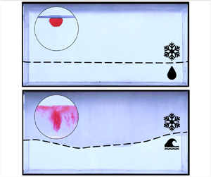
Sea water freezing modes in a natural convection system

Published online by Cambridge University Press:  11 April 2023

Yihong Du
Affiliation:
Center for Combustion Energy, Key Laboratory for Thermal Science and Power Engineering of MoE, International Joint Laboratory on Low Carbon Clean Energy Innovation, and Department of Energy and Power Engineering, Tsinghua University, 100084 Beijing, PR China
Ziqi Wang
Affiliation:
Center for Combustion Energy, Key Laboratory for Thermal Science and Power Engineering of MoE, International Joint Laboratory on Low Carbon Clean Energy Innovation, and Department of Energy and Power Engineering, Tsinghua University, 100084 Beijing, PR China
Linfeng Jiang
Affiliation:
Center for Combustion Energy, Key Laboratory for Thermal Science and Power Engineering of MoE, International Joint Laboratory on Low Carbon Clean Energy Innovation, and Department of Energy and Power Engineering, Tsinghua University, 100084 Beijing, PR China
Enrico Calzavarini*
Affiliation:
Univ. Lille, Unité de Mécanique de Lille – J. Boussinesq (UML) ULR 7512, F-59000 Lille, France
Chao Sun*
Affiliation:
Center for Combustion Energy, Key Laboratory for Thermal Science and Power Engineering of MoE, International Joint Laboratory on Low Carbon Clean Energy Innovation, and Department of Energy and Power Engineering, Tsinghua University, 100084 Beijing, PR China Department of Engineering Mechanics, School of Aerospace Engineering, Tsinghua University, Beijing 100084, PR China
*
Email addresses for correspondence: enrico.calzavarini@univ-lille.fr, chaosun@tsinghua.edu.cn

Abstract

Sea ice is crucial in many natural processes and human activities. Understanding the dynamical couplings between the inception, growth and equilibrium of sea ice and the rich fluid mechanical processes occurring at its interface and interior is of relevance in many domains, ranging from geophysics to marine engineering. Here we investigate experimentally the complete freezing process of water with dissolved salt in a standard natural convection system, i.e. the prototypical Rayleigh–Bénard cell. Due to the presence of a mushy phase, the studied system is considerably more complex than the freezing of fresh water in the same conditions (Wang et al., Proc. Natl Acad. Sci. USA, vol. 118, issue 10, 2021, e2012870118). We measure the ice thickness and porosity at the dynamical equilibrium state for different initial salinities of the solution and temperature gaps across the cell. These observables are non-trivially related to the controlling parameters of the system as they depend on the heat transport mode across the cell. We identify in the experiments five out of the six possible modes of heat transport. We highlight the occurrence of brine convection through the mushy ice and of penetrative convection in stably stratified liquid underlying the ice. A one-dimensional multi-layer heat flux model built on the known scaling relations of global heat transport in natural convection systems in liquids and porous media is proposed. Given the measured porosity of the ice, it allows us to predict the corresponding ice thickness, in a unified framework.

Type
JFM Papers
Copyright
© The Author(s), 2023. Published by Cambridge University Press

1. Introduction

The evolution of sea ice has important impacts on many environmental and geological processes as well as human activities. Examples include ocean circulation (Clark, Alley & Pollard Reference Clark, Alley and Pollard1999; Joughin, Alley & Holland Reference Joughin, Alley and Holland2012; Hanna et al. Reference Hanna2013; Straneo & Heimbach Reference Straneo and Heimbach2013; Stevens et al. Reference Stevens, Hulbe, Brewer, Stewart, Robinson, Ohneiser and Jendersie2020), global sea-level rise (Wadhams & Munk Reference Wadhams and Munk2004), land-surface albedo (Curry, Schramm & Ebert Reference Curry, Schramm and Ebert1995; Perovich et al. Reference Perovich, Grenfell, Light and Hobbs2002; Scagliarini et al. Reference Scagliarini, Calzavarini, Mansutti and Toschi2020), biodiversity (Post et al. Reference Post, Bhatt, Bitz, Brodie, Fulton, Hebblewhite, Kerby, Kutz, Stirling and Walker2013), microplastic dispersion and sequestration (Peeken et al. Reference Peeken, Primpke, Beyer, Gütermann, Katlein, Krumpen, Bergmann, Hehemann and Gerdts2018; Obbard et al. Reference Obbard, Sadri, Wong, Khitun, Baker and Thompson2014), and winter navigation at high latitudes and polar areas (de Andrés, Saarinen & Uuskallio Reference de Andrés, Saarinen and Uuskallio2018; Ho Reference Ho2010). Generally, sea ice evolution is associated with the complex fluid dynamic processes occurring in the oceans that involve wide ranges of spatial and temporal scales. Their descriptions through numerical models in the geophysical context make use of so-called micro-scale physical parametrizations that have a key role in the reliability and accuracy of the resulting predictions (Rae et al. Reference Rae, Hewitt, Keen, Ridley, West, Harris, Hunke and Walters2015; Rousset et al. Reference Rousset2015).

In this study, we focus on the role of buoyancy-driven natural convection in determining upper-surface sea ice growth and the attainment of dynamical equilibrium. We do this by performing experiments at the laboratory scale in a highly controllable setting, the Rayleigh–Bénard cell (see below). With this approach, we aim at providing a highly reliable small-scale parametrization of the process that is crucial for geophysical-scale computational models in the wide range of applications mentioned above.

The Rayleigh–Bénard (RB) system, a fluid layer parallelly confined between a warmer horizontal bottom plate and a cooler top plate, and insulated on the lateral sides (Ahlers, Grossmann & Lohse Reference Ahlers, Grossmann and Lohse2009; Lohse & Xia Reference Lohse and Xia2010; Chillà & Schumacher Reference Chillà and Schumacher2012), is a paradigmatic model system in the physics of nonlinear systems and fluid mechanics. Its behaviour has been studied for decades, and it has been crucial in developing the understanding of hydrodynamic instabilities, transition to chaos, turbulence and turbulent transport. Its local and global properties across its wide spectrum of regimes are nowadays well-characterized (Ahlers et al. Reference Ahlers, Grossmann and Lohse2009; Chillà & Schumacher Reference Chillà and Schumacher2012). More recently, the RB system has been proven to be also convenient for studying the couplings between liquid–solid phase change and fluid flow phenomena (Esfahani et al. Reference Esfahani, Hirata, Berti and Calzavarini2018; Favier, Purseed & Duchemin Reference Favier, Purseed and Duchemin2019). It has a laboratory scale, it is closed, and in/out energy fluxes can be measured, hence it is highly controllable, yet able to reproduce the rich process of water freezing in the presence of unsteady and turbulent flow conditions. Several recent studies have investigated the influence of temperature (Wang et al. Reference Wang, Calzavarini, Sun and Toschi2021c; Yang et al. Reference Yang, Howland, Liu, Verzicco and Lohse2023b), inclination (Wang et al. Reference Wang, Jiang, Du, Sun and Calzavarini2021d; Yang et al. Reference Yang, Chong, Liu, Verzicco and Lohse2022), rotation (Ravichandran, Toppaladoddi & Wettlaufer Reference Ravichandran, Toppaladoddi and Wettlaufer2022), initial conditions, and aspect ratio (Wang, Calzavarini & Sun Reference Wang, Calzavarini and Sun2021b) on fresh water freezing/melting in the RB system. However, the presence of dissolved salt in sea water adds to the complexity of the processes. In particular, two factors need to be considered to properly study the evolution of sea ice.

The first factor is the mushy structure of sea ice (Feltham et al. Reference Feltham, Untersteiner, Wettlaufer and Worster2006), which allows for the occurrence of interstitial fluid motion, i.e. brine drainage and thermal convection across the sea ice. Various studies have discussed the mushy structure forming in the solidification of aqueous solutions. The focus has mainly been on onset conditions for convective brine drainage (Wettlaufer, Worster & Huppert Reference Wettlaufer, Worster and Huppert1997), mushy phase morphology (Peppin, Huppert & Worster Reference Peppin, Huppert and Worster2008), ice layer growth rate (Kerr et al. Reference Kerr, Woods, Worster and Huppert1990), ice porosity (Wettlaufer et al. Reference Wettlaufer, Worster and Huppert1997), flow structure within the mushy phase (Chen Reference Chen1995; Worster & Wettlaufer Reference Worster and Wettlaufer1997), and salinity in the liquid phase (Wettlaufer et al. Reference Wettlaufer, Worster and Huppert1997; Peppin et al. Reference Peppin, Huppert and Worster2008). While these studies together with relevant reviews (Worster Reference Worster1997; Wells, Hitchen & Parkinson Reference Wells, Hitchen and Parkinson2019; Anderson & Guba Reference Anderson and Guba2020) provide a detailed, thorough and multi-perspective understanding of brine drainage and mushy phase structure, the interactions between the mushy structure and a neighbouring vigorous thermal convective flow are much less explored. A few studies discussing the growth of sea ice focus either on establishing governing momentum and energy equations suitable for numerical simulations (Feltham et al. Reference Feltham, Untersteiner, Wettlaufer and Worster2006; Covello et al. Reference Covello, Abba, Bonaventura, Della Rocca and Valdettaro2016; Wells et al. Reference Wells, Hitchen and Parkinson2019), or on theoretical models that view ice growth as purely diffusion controlled (Notz Reference Notz2005; Worster & Rees Jones Reference Worster and Rees Jones2015).

The second factor is salty water's peculiar equation of state, in particular its density dependence on salinity and temperature (Gebhart & Mollendorf Reference Gebhart and Mollendorf1977), and its freezing point depression (Bodnar Reference Bodnar1993). While for normal sea water with 3.5 % salinity (i.e. the mass concentration of dissolved salt), the density decreases monotonically as the temperature is increased from its freezing point, this is not the case for less salty water (encountered, for instance, near river estuaries) or fresh water, where a maximal density occurs in the interval $[0,4]\,^{\circ }$C (Lyman & Fleming Reference Lyman and Fleming1940; Pawlowicz Reference Pawlowicz2015). Salty water's peculiar density dependence may lead to different combinations of stable/unstable stratifications of the liquid phase in the RB cell. In a similar yet simpler scenario, the combination of stable stratification and unstably stratified turbulence has been found to have a significant influence on the freezing dynamics and equilibrium ice thickness of fresh water (Townsend Reference Townsend1964; Wang et al. Reference Wang, Calzavarini, Sun and Toschi2021c). Other studies point out that the kind of stratification, either stable or unstable, in touch with the melting front has a key role in determining the melting rate of a pure-ice layer in aqueous solutions (Sugawara & Irvine Reference Sugawara and Irvine2000; Mondal et al. Reference Mondal, Gayen, Griffiths and Kerr2019; Rosevear, Gayen & Galton-Fenzi Reference Rosevear, Gayen and Galton-Fenzi2021; Yang et al. Reference Yang, Howland, Liu, Verzicco and Lohse2023a). However, these studies focus on stratifications due to the salinity gradient in double-diffusive convection with linearized equation of state salt–water mixtures, i.e. neglecting the above-mentioned important nonlinear dependencies of density with respect to temperature and salinity.

In this work, we investigate how ice growth and fluid dynamics in salty water couple and co-evolve until the equilibrium in the RB natural convection system is reached. We aim to reveal how sea ice growth rate depends on controlled environmental conditions through its interactions with mushy phase convection and with the variety of density stratification patterns and fluid flows occurring in the underlying liquid phase.

The paper is organized as follows. Section 2 describes the experimental set-up and the measurement methodology. Section 3 describes the experimental results, focusing on the growth dynamics and equilibrium morphology of the ice layer. To provide a first-step understanding of the complex process, in § 4 we discuss how the equilibrium ice thickness, its porosity and the saturation time depend on temperature and salinity conditions, as well as the correlation among these global properties. Section 5 introduces a one-dimensional multi-layer heat flux model that describes the equilibrium ice thickness's dependence on the system control parameters, and identifies five out of six possible modes of heat transport in the experimental system. Finally, we end with conclusions and outlook in § 6.

2. Experiments

The experiments are performed in a rectangular cuboid RB cell (height $H=0.12$ m, aspect ratio $\varGamma = L/H = 2$, width–height ratio $W/H = 0.5$, i.e. a so-called quasi-two-dimensional system). An expansion vessel is attached to compensate for the volume change during the freezing process and so to monitor the mushy phase growth; see figure 1(a). The top and bottom plate temperatures are measured with thermistors and controlled with circulating baths. Sidewalls are isolated with foam material to approach ideal adiabatic boundary conditions. The cell is initially filled with degassed salty water of initial salinity $S_i$. Here, we use sodium chloride (NaCl), the principal solute of sea water (Lyman & Fleming Reference Lyman and Fleming1940), as the salt, and $S_i$ is varied from 0 % (fresh water) to 3.5 % (average ocean salinity), with the corresponding freezing point $T_{0i}$ (Hall, Sterner & Bodnar Reference Hall, Sterner and Bodnar1988) varying from $0^{\circ }$C to $-2.1\,^{\circ }$C. The (hot) bottom plate temperature $T_b$, which is equal to the initial liquid temperature, ranges from $0.4^{\circ }$C to 12.9 $^{\circ }$C, and the (cold) top plate temperature $T_t$ is set 10 K below the freezing temperature, hence $T_t = T_{0i}-10$ K (from $-10^{\circ }$C to $-12.1\,^{\circ }$C, depending on $S_i$). A dimensionless bottom superheat parameter can then be defined as $\varTheta _i = (T_b-T_{0i})/(T_b-T_t)$. This parameter characterizes the initial ratio of the admissible temperature difference in the liquid phase over the total gap across the cell. It can also evolve slightly during the experiment. This is because the melting temperature depends on the actual salinity, and at the equilibrium state, $S_e$ and so $T_{0e}$ might differ from the initial values (actually $S_e$ can be as high as $7\,\%$, with $T_{0e}\approx -4.2\,^{\circ }$C; see figure 5b). Since the total quantity of solute is constant, one expects an enhancement of salinity in the liquid due to salt ejection from the mush (and so an increase of $\varTheta$).

Figure 1. Sketch of the experimental system and temperature–salinity parameter space. (a) Cartoon of the experimental set-up. The height of the cell is $H=0.12$ m, the aspect ratio is $\varGamma = L/H = 2$, and the width–height ratio is $W/H = 0.5$. An expansion vessel is attached to compensate for the volume change and to monitor the ice/mushy phase growth. The bottom plate temperature is kept at $T_b$, and the top plate temperature $T_t$ is maintained at 10 K below the freezing point $T_{0i}$ at the initial salinity $S_i$. A dimensionless bottom superheat parameter is defined as $\varTheta _i=(T_b-T_{0i})/(T_b-T_t)$. (b) Temperature–salinity parameter space. In this work, we test $\varTheta _i$ values $1/5$ (purple), $1/3$ (red), $3/8$ (green), $3/7$ (pink), $1/2$ (blue) and $3/5$ (brown). The initial salinity $S_i$ varies from 0 % to 3.5 %; $T_b$ (dots) is shown for each case. We also plot $T_{0i}$ (black squares) and $T_t$ (grey triangles) as functions of $S_i$.

In this work, we first test the states with $\varTheta _i$ values $1/3$, $3/8$ and $1/2$ with salinities $S_i \in [0, 3.5]\%$. Cases with $\varTheta _i$ values $1/5$, $3/7$ and $3/5$, and $S_i = 3.5$%, are also performed to test the results in a wider temperature range. A visualization of the temperature–salinity parameter space explored in the experiments is provided in figure 1(b). It reports the temperature values $T_b$, $T_{0i}$ and $T_t$ for different $\varTheta _i$ and $S_i$. In this experimental configuration, the ice/mushy phase grows from the top plate until the system reaches an equilibrium. We assume that this state is attained when the mean mushy phase thickness $h(t)$ (see figure 1a) changes less than 1 % in eight hours, with the maximum experiment duration being three days. The ice or mushy phase thickness and its porosity $\phi (t)$ (i.e. the volume fraction of residual liquid in the ice or mushy phase) can be obtained, respectively, by identifying the ice–liquid interface in photos of the system, and by using the expansion vessel readings together with the assumption of total mass conservation in the system. The evaporation from the expansion vessel is negligible as it causes only a mass loss less than 0.1 % of the total mass of the system. We refer to Appendix A for more details on the measurement protocols.

3. Mushy phase morphology and growth dynamics

Figures 2(a,c) show photos of the experiment at its equilibrium state in two typical cases ($S_i=0$, 3.5 % and $\varTheta _i=3/8$). One can readily appreciate the different thicknesses of the iced domains (thinner in the salty water case) and the different interface shapes between the two cases. However, their dissimilarity is not only volumetric and morphological, but also structural. To illustrate this, we hollowed out a tiny (5 mm) hemispherical cavity on the top horizontal surface of the ice matrix on which we deposited a drop of red dye. Figures 2(b,d) show two lateral view photos of the stain after 5 min to form its deposition. We observe that when $S_i=0$ (figure 2b), the iced phase is transparent and the dye does not spread into it, indicating the dense structure of the matrix. On the contrary, at $S_i=3.5\,\%$ (figure 2d), the iced phase looks opaque and the dye spreads anisotropically, which highlights a complex porous medium filled with liquid (i.e. a mushy phase structure) with internal vertical channels.

Figure 2. Images of the iced layer together with its internal structure, and evolution of the freezing front. (ad) Photos of ice/mushy phases without (a,b) and with (c,d) porosity. The experimental conditions are (a,b) $S_i=0\,\%$, and (c,d) $S_i=3.5\,\%$, both with $\varTheta _i = 3/8$. In (b,d), the red dye of the same amount and concentration is deposited into a small hemispherical pit carved at the same location on the upper surface of the corresponding solid matrix in (a,c). The ice in (a,b) is transparent, and the dye does not spread. The mushy phase with porosity in (c,d) is relatively opaque, and the dye spreads anisotropically, possibly indicating the presence of channels. (e) Dynamics of the freezing front. The mushy phase thicknesses $h(t)$, non-dimensionalized by $H$, are plotted as functions of time non-dimensionalized by the diffusive time scale $t^* =H^2/\kappa _{ice}=1.22\times 10^4$ s (where $\kappa _{ice}$ is ice thermal diffusivity) for three experimental runs. (f) The same data as in (e) are compensated by the diffusive behaviour $h(t)/\sqrt {t}$ (normalized by the first data to compare different cases).

It is noteworthy that the different iced phase structures correspond to different freezing dynamics. This is well illustrated in figures 2(e,f), where the temporal growth of the freezing front, $h(t)$, is shown for three sets of experimental conditions, corresponding to pure water, intermediate salinity and sea water salinity, all at $\varTheta _i=3/8$. Though all three cases display an initial period of diffusive ice phase growth, i.e. $h \propto \sqrt {t}$, later the growth rate decreases for the case $S_i=0$, 2 %; while when $S_i=3.5\,\%$, the instantaneous growth rate increases and even exceeds the diffusive growth rate before reaching the equilibrium. It is remarkable also to note that the equilibrium height is not simply proportional to the salinity. The above highlighted temporal evolution of the ice growth in a salty solution depends on the internal structure of the mushy phase that in turn might also change in time (e.g. due to the formation of brine channels Wettlaufer et al. Reference Wettlaufer, Worster and Huppert1997; Worster & Wettlaufer Reference Worster and Wettlaufer1997). A quantitative description of this process is challenging because it requires detailed knowledge of the mushy microstructure. The same is true for any attempt to characterize the morphology of the solid–fluid interface. For this reason, in the following we focus on a simpler question: we try to tackle the globally averaged equilibrium state that is reached asymptotically in time. In other words, we aim at understanding the factors that control the average thickness, denoted $h_e$, of the iced mushy phase.

4. Global properties of the equilibrium state

We display in figure 3 two important spatially averaged properties of the mushy phase at the equilibrium (from now on denoted with a subscript $e$): they are the dimensionless thickness $h_e/H$ and the porosity $\phi _e$. Besides this, we report the saturation time (or time to equilibrium) denoted as $t_{e}^{90\,\%}$, here for practical reasons defined as the time it takes to reach 90 % of the equilibrium thickness non-dimensionalized by the diffusive time scale $t^*=H^2/\kappa _{ice}=1.22\times 10^4$ s. The dependence of the thickness $h_e$ as a function of the initial salinity $S_i$ is very different for distinct values of the control parameter $\varTheta _i$ (see figure 3a): $h_e$ exhibits a similar non-monotonic (decrease–increase–decrease) pattern for $\varTheta _i = 1/3, 3/8$, and is monotonically decreasing for $\varTheta _i = 1/2$. These trends are in part reflected on the $\phi _e(S_i)$ dependence, which presents considerable fluctuations for intermediate salinity values, although its overall trend is increasing for all $\varTheta _i$ cases (see figure 3b).

Figure 3. Global properties of the equilibrium state from experiments. The initial superheats are respectively $\varTheta _i$ values $1/3$ (red), $3/8$ (green) and $1/2$ (blue), and the initial salinity $S_i$ varies from 0 % to $3.5\,\%$. The error bars are measured by repeated experiments in two cases with $S_i = 3.5\,\%$ and $\varTheta _i = 1/3$, $1/2$, respectively. (a) The mean mushy phase thickness $h_e$ initially decreases with $S_i$ for all three superheats, and is followed by a sharp increase for the $\varTheta _i = 1/3$ and $3/8$ cases. The shaded areas indicate the minimal and maximal spatial variations of mushy phase thicknesses. The thicknesses are non-dimensionalized by $H$. (b) The mean mushy phase porosity $\phi _e$ exhibits a non-monotonic yet overall increasing trend with $S_i$. (c) Thickness $h_e$ does not exhibit a statistically strong correlation with $\phi _e$. (d) The saturation time $t_e^{90\,\%}$ is defined as the time to reach 90 % of the equilibrium mushy phase thickness $h_e$, and is non-dimensionalized by the diffusive time scale $t^*=1.22\times 10^4\,{\rm s}$. The variations of $t_{e}^{90\,\%}$ with $S_i$ are consistent with those of $h_e$. (e) Thickness $h_e$ shows a clear positive correlation with $t_{e}^{90\,\%}$. A linear fitting gives $h_e/H = 0.0912 \times t_{e}^{90\,\%}/t^*$ (dash-dot line), with correlation coefficient $R^2=0.9846$.

The fact that a more porous ice matrix (high $\phi _e$) can release more salt into the liquid and as a consequence lower the final freezing point of the solution, $T_{0e}$, hence reducing the size of $h_e$, might give a rationale for the globally observed trends. However, this alone is not enough to explain any of the observed fluctuations or non-monotonic dependencies in $h_e$ and $\phi _e$. Moreover, it is important here to notice that the existence of a correlation between $\phi _e$ and $h_e$ is not evident from the present measurements (see figure 3c). If, for instance, mass conservation and geometry were simply ruling the relation between the equilibrium mushy layer thickness and the mushy layer porosity, then one would have $h_e(1-\phi _e) = const.$ (where the constant represents the height of the ice layer in the case of zero salinity and correspondingly no porosity). This implies an increasing trend of $h_e$ with $\phi _e$, while figure 3(c) suggests just the opposite (one can notice a decreasing $h_e(\phi _e)$ for fixed values of $\varTheta _i$). We conclude that the $h_e(\phi _e$) relation is a non-trivial function of the system control parameters $S_i$ and $\varTheta _i$.

Finally, we observe that the trends for $t_{e}^{90\,\%}$ are instead consistent with those of $h_e$ (figure 3d), and a clear linear correlation can be seen between the two quantities (figure 3e). This correspondence can provide a way to estimate the time to equilibrium just by focusing on the magnitude of $h_e$. Therefore, in the following, we will focus on modelling the physical mechanisms responsible for the variations of $h_e$. The question that we wish to address is: can the equilibrium global properties be understood in terms of a model that considers just (i) the role of porosity, and (ii) the role of thermal stratification, on the steady state of the heat transfer process in the system, without taking into account its complex transient dynamics?

5. Multi-layer heat flux model

To answer the above question, we need to understand how $h_e$ and $\phi _e$ are related and how the heat transport across the system is influenced by the convection in the mushy phase and by the combination of stable stratification and unstably stratified turbulence. We will show that a one-dimensional (or integral) multi-layer heat flux model that relies on scaling laws known for natural convection in fluid and porous media can explain $h_e$ with good accuracy once $\phi _e$ is provided as input from the experiment. On the other hand we observe that a quantitative description of $\phi _e$ requires a model for the evolution of the microscopic structure of the porous ice matrix. This is a challenging task that currently goes beyond our capabilities and that we leave for future research. In summary, the multi-layer heat flux model presented in the following allows us to explain the complex relation linking $h_e$ and $\phi _e$, when the latter is considered as an independent variable.

We assume that the position of the solid–fluid interface in the system at the equilibrium $h_e$ is the result of the balance between the mean heat flux across the mushy phase, $\mathcal {F}_m$, and the one in the liquid, $\mathcal {F}_l$ (see figure 4). Both these quantities require a parametrization, which we detail in the following. For conciseness and better readability, we refer the reader to table 1 in Appendix D for the denomination of the many physical quantities and material properties involved in the model.

Figure 4. Synoptic representation of the averaged multi-layer heat flux model. Row 1 provides the adopted parametrization for the global heat flux expression in the mushy phase, $\mathcal {F}_m$, together with the definitions of $Nu_m$ and $Ra_m$. Rows 2–4 report the expression for the global heat flux in the liquid phase, $\mathcal {F}_l$, together with the $Nu_l$ and $Ra_l$ definitions (column 4). Three different combinations of stratifications may exist: (a) unstable, (b) mixed, (c) unstable. The discriminating criterion for their occurrence is the monotonicity of liquid density within the temperature range $[T_{0e}, T_b]$, i.e. the relative magnitude of $T_{0e}$, $T_b$ and the maximum-density temperature $T_{max}$ (column 2), which depends on the salinity $S_e$. Column 3 gives the sketches of these combinations, together with the layer thicknesses and the interface temperatures. The colour gradient indicates the density gradient in the liquid phase, with red representing lighter liquid, and blue representing heavier liquid. The model is supplemented with five input parameters, $T_t$, $T_b$, $S_i$, $\phi _e$ and $H$, and leads to an estimation of $h_e$ (row 5) through the assumption of a statistically steady heat flux balance among layers.

Table 1. Symbols used in this paper.

We express the heat flux across the mushy phase in the statistically steady condition in the form

(5.1)\begin{equation} \mathcal{F}_m = Nu_m \, \varLambda _m(T_m)\,\frac{T_t-T_{0e}}{h_e}. \end{equation}

Equation (5.1) involves the mushy phase Nusselt number $Nu_m$, i.e. the ratio between the total and the conductive heat transfer across the mushy phase. Its dependence as a function of the Rayleigh number $Ra_m$ is known from previous studies on convection in porous media. Here, we use the parametrization by Gupta & Joseph (Reference Gupta and Joseph1973):

(5.2)\begin{equation} Nu_m=\left\{ \begin{array}{@{}ll} 1 , & Ra_m < Ra_{mcr}, \\[2pt] 1.3338+0.0099\,Ra_m, & Ra_m \ge Ra_{mcr}, \end{array} \right . \end{equation}

where the mushy-critical Rayleigh number is $Ra_{mcr}=4{\rm \pi} ^2$. The Rayleigh number for the flow in a porous medium is defined as

(5.3)\begin{equation} Ra_m=\frac{ \varPi \it}{\phi_e}\,\frac{g( \rho(S_t, T_t)- \rho(S_e, T_{0e}))h_e}{\nu(T_m)\,\kappa(T_m)\, \rho(S_e, T_m)}. \end{equation}

This definition involves the evaluation of the permeability $\varPi$, a quantity describing the conductivity of a porous medium to fluid flow (Pal, Joyce & Fleming Reference Pal, Joyce and Fleming2006). The permeability is a function of the structure of the porous ice matrix and is notoriously difficult to measure, in particular for ice, because it is highly sensitive to the environmental conditions and to the history of the medium. Several previous studies, including Kawamura et al. (Reference Kawamura, Ishikawa, Takatsuka, Kojima and Shirasawa2006), Petrich, Langhorne & Sun (Reference Petrich, Langhorne and Sun2006) and Polashenski et al. (Reference Polashenski, Golden, Perovich, Skyllingstad, Arnsten, Stwertka and Wright2017), revealed that there exists a threshold porosity ($\phi _c$) below which the ice behaves as impermeable. Above such a threshold, the permeability is well approximated by a power-law function of the porosity. We adopt here a similar functional parametrization to relate $\varPi$ to $\phi _e$:

(5.4)\begin{equation} \varPi=\left\{ \begin{array}{@{}ll} 0 , & \phi_e < \phi_{cr}, \\[2pt] C(\phi_e - \phi_{cr})^\alpha, & \phi_e \ge \phi_{cr}, \end{array} \right. \end{equation}

where the three adjustable parameters are chosen as $C=7 \times 10^{-8}$ m$^2$, $\alpha =3$ (as at the leading order of the Carmen–Kozeny relation; Wells et al. Reference Wells, Hitchen and Parkinson2019) and $\phi _{cr}=0.054$ to best fit $h_e$ measured experimentally. Although these values are ad hoc for our study, the modelled $\varPi$ is of the same order of magnitude as the ones reported in sea ice laboratory and field researches (Kawamura et al. Reference Kawamura, Ishikawa, Takatsuka, Kojima and Shirasawa2006; Petrich et al. Reference Petrich, Langhorne and Sun2006; Polashenski et al. Reference Polashenski, Golden, Perovich, Skyllingstad, Arnsten, Stwertka and Wright2017).

Similarly, the mean heat flux in the liquid phase can be expressed in the approximate form

(5.5)\begin{equation} \mathcal{F}_l = \left\{ \begin{array}{@{}ll} Nu_l \, \varLambda_l(T_l)\,\dfrac{T_{0e}-T_b}{H-h_e}, & T_{max} \le T_{0e}, \\ \varLambda_l(T_s)\,\dfrac{T_{0e}-T_{max}}{h_{max}} = Nu_l \, \varLambda_l(T_u)\,\dfrac{T_{max}-T_b}{H-h_e-h_{max}}, & T_{max}\in (T_{0e},T_b),\\ \varLambda_l(T_l)\,\dfrac{T_{0e}-T_b}{H-h_e}, & T_{max} \ge T_b. \\ \end{array} \right . \end{equation}

Note that the above expression is composed of three distinct cases according to the value, $T_{max}$, of the temperature corresponding to the maximal density of the liquid solution at the equilibrium with respect to $[T_{0e}, T_b]$. This reflects in three distinct cases: (a) unstable stratification, (b) a stable layer above an unstable one, and (c) a single stable layer; see figure 4. The scale $h_{max}$, appearing in case (b), is the height of the stably stratified layer in the intermediate case. It can be determined by equating the two fluxes across the stable and unstable layers of liquid. The dimensionless heat flux in the liquid is accounted for by the Nusselt number $Nu_l$, dependent on the Rayleigh number $Ra_l$, a relation that is relatively well known. Wang et al. (Reference Wang, Calzavarini, Sun and Toschi2021c) proposed the parametrization below by fitting the data from their simulations on the freezing of fresh water in an RB convection system, which leads to theoretical predictions agreeing well with their experiment results. The same parametrization is adopted in the present study:

(5.6)\begin{equation} Nu_l =\left\{ \begin{array}{@{}ll} 1 , & Ra_l < Ra_{lcr}, \\ 0.12+0.88\,Ra_l / Ra_{lcr}, & Ra_l \in [Ra_{lcr}, 1.23\,Ra_{lcr}], \\ 0.27(Ra_l -Ra_{lcr})^{0.27}, & Ra_l > 1.23\,Ra_{lcr}, \end{array} \right . \end{equation}

where the critical Rayleigh number for the onset of convection is $Ra_{lcr}=1708$. We note that the definition of the Rayleigh number in the liquid is needed only for the two cases that involve a density unstable stratification (cases (a) and (b) in figure 4). We use

(5.7)\begin{equation} Ra_{l} = \left\{ \begin{array}{@{}ll} \dfrac{g( \rho(S_e, T_{0e})- \rho(S_e, T_b))( H-h_e )^3 }{\nu(T_l)\,\kappa(T_l)\,\rho(S_e, T_l)}, & T_{max}\le T_{0e},\\ \dfrac{g( \rho(S_e, T_{max})- \rho(S_e, T_b))( H-h_e-h_{max}) ^3 }{\nu(T_u)\,\kappa(T_u)\,\rho(S_e, T_u)}, & T_{max}\in (T_{0e},T_b). \end{array} \right . \end{equation}

Finally, the model tuning requires the numerical values of material properties (see Appendix C for the empirical formulas adopted), which are evaluated at the equilibrium salinity $S_e$. Given the facts that in the present system no salinity source exists, that liquid in the mushy phase contains only a small salt fraction, and that salt is mixed in the liquid either vigorously by convection or slowly by diffusion, we can assume that $S_e$ is uniform in the liquid layer. Hence $S_e$ can be related implicitly to $h_e$ and the inputs of the model by the mass conservation of the salt:

(5.8)\begin{equation} S_e\,\rho(S_e, T_{mean})\,(H-h_e(1-\phi_e))=S_i\,\rho(S_i, T_{b})\,H. \end{equation}

It is worth noticing that (5.8) is suitable only for the present system (when applied to other systems, e.g. open systems, a measurement of $S_e$ must be supplied). The evaluation of $Ra_m$ requires also the value of $\rho (S_t, T_t)$. While $T_t$ is known as it is imposed externally, $S_t$ is not. We assume here that the latter takes the value such that $T_t$ is a local freezing point, $T_0(S_t)=T_t$; in other words, we assume local thermodynamical equilibrium within the mushy phase (Wells et al. Reference Wells, Hitchen and Parkinson2019). Finally, by solving simultaneously the algebraic equations of heat flux balance $\mathcal {F}_m = \mathcal {F}_l$ and the mass conservation of the salt (5.8), using the measured value $\phi _e$, the model leads to the equilibrium mushy phase thickness $h_e$. We refer to Appendix B for a more detailed explanation of how the model is implemented numerically.

The model results are all illustrated in figure 5. Figure 5(a) shows the mean mushy phase thickness $h_e/H$ as a function of $S_i$ together with its comparison with the experiment results. At $\varTheta _i=1/2$ (blue lines and symbols), where ice thickness decreases for increasing salinity, the agreement with the model is fairly good. The model suggests that in this condition, the heat transfer through the mushy phase remains diffusive (mushy diffusion, MD state). Increasing the salinity, the freezing point is lowered, and this slightly reduces the frozen layer thickness. The role of porosity is marginal as here it stays approximately constant with $S_i$ (see figure 3b). For $\varTheta _i=1/3$ and $3/8$ (red and green lines and symbols), the non-monotonic behaviour is also captured by the model.

Figure 5. Model results for ice/mushy phase thickness compared with the experiments, and identification of heat transport modes. MD/MC stand for diffusive/convective heat transfer in the mushy phase; similarly, LD/LC stand for diffusive/convective heat transport in the liquid phase, while LPC stands for diffusive and convective heat transport due to penetrative convection in the liquid phase, i.e. a combination of diffusive and convective heat transport, as a stable stratification lies above an unstable one. (a) The initial superheat values are respectively $\varTheta _i$ values $1/3$ (red), $3/8$ (green) and $1/2$ (blue), and the initial salinity $S_i$ varies from 0 % to $3.5\,\%$. The calculated $h_e$ (lines with open circles) is close to the experimental results (dots). The spatial variations of mushy phase thicknesses from the experiments (shaded areas) are also included, together with results of reduced models ignoring mushy phase convection ($Nu_m \equiv 1$, dash-dot lines) and ignoring liquid stratification (linear density dependence on temperature $\rho (S_e, T)=\rho (S_e, T_b)\,(1-\beta (S_e, T_b)\,(T-T_b))$, dash-double-dot lines). (b) Phase space diagram based on the two effective control parameters $Ra_m$ and $Ra_l$. The third effective control parameter $S_e$ is not presented as an axis, for readability. Instead, different circle sizes are used to distinguish the different $S_e$. There are in total six heat transport modes of the system. Our experiments fall within five cases. Different circle colours are used to distinguish different $\varTheta _i$. The highest salinity ($S_e \gtrsim 2.7\,\%$) is expected to suppress the LPC regime as it removes the density anomaly of the solution. (cg) Images from the experiment for typical cases corresponding to the five observed heat transport modes.

It is relevant here to also consider two reduced versions of the model, one ignoring the occurrence of convection in the mushy phase (by assuming $Nu_m \equiv 1$, dash-dot lines in figure 5a), the other neglecting the non-monotonic density stratification in the liquid phase (by assuming linear density dependence on temperature, i.e. $\rho (S_e, T)=\rho (S_e, T_b)\,(1-\beta (S_e, T_b)\,(T-T_b))$, where $\beta (S_e, T_b)$ is the liquid thermal expansion coefficient at the bottom plate, dash-double-dot lines). The comparison of the calculated $h_e$ stemming from the two reduced models allows us to interpret the ‘jump’ or sudden increase in the ice thickness as being associated with the occurrence of convection in the mushy phase (mushy convection, MC state) with increased $\phi _e$ (see figure 3b). Convection strengthens the heat transport, promoting a larger mushy phase growth rate, because $\text {d}h/\text {d}t \propto \mathcal {F}_m - \mathcal {F}_l$. The equilibrium mushy layer thickness, as a result of the competitive balance between $\mathcal {F}_m$ and $\mathcal {F}_l$, also increases because of the enhanced heat transfer efficiency in the mushy phase.

However, the mushy phase convention alone is not sufficient to explain the tendency of $h_e$ (see the dash-double-dot lines in figure 5a). Especially large deviations from experiment results can be seen when $S_i$ is low as they fall into LD (liquid diffusion) and LPC (liquid penetrative convection) regimes (see figure 5b). In the LD state, only diffusive heat transport occurs in the liquid phase, either because the whole liquid phase is stably stratified or because the liquid phase is too thin to support convection. In the LPC state, there is always a stable stratification in contact with the mushy phase above the unstably stratified turbulence, also known as penetrative convection. The presence of this stable layer limits the below convective motion and prevents the mushy phase from a direct penetration of the convection. As an effect, the heat transport across the liquid phase is relatively low, enabling the mushy phase to grow thick. When $S_i$ is increased, the temperature differences decrease in the stably stratified region (from $T_{0e}$ to $T_{max}$) and increase in the unstably stratified turbulence (from $T_{max}$ to $T_b$). As a consequence, the convective motion intensifies, becoming even more turbulent, leading to strong heat transport across the liquid phase and so decreasing $h_e$. Similarly, the temperature difference in the unstable stratification is smaller when $\varTheta _i$ is lower. The unstably stratified turbulence is weaker, and the thermal resistance in the stable stratification above plays a more important role in determining the heat transport of the whole liquid phase. This accounts for the relatively larger errors between the dash-double-dot lines (assuming the entire liquid phase to be unstably stratified) and the experiment results in figure 5(a) when $\varTheta _i= 1/3$ and $3/8$, compared to cases with $\varTheta _i= 1/2$ and the same $S_i$. By further increasing $S_i$, the stable stratification layer disappears, and the heat transport in the liquid phase is purely convective (liquid convection, LC state; see figure 5b).

The remaining discrepancies between the model and the experiments are likely to be related to the modelling of the mushy phase, in particular from neglecting its non-homogeneous internal structure and the uncertainties in the parametrization of its permeability. It is also worth mentioning that the heat transport in the LPC regime can also be clearly described by means of two alternative parameters introduced in Wang et al. (Reference Wang, Reiter, Lohse and Shishkina2021a). They are the so-called density inversion parameter (which here reads $(T_{max}-T_{0e})/(T_b-T_{0e})$) and the Rayleigh number relative to the whole fluid layer. It is an alternative but equivalent approach with respect to the one adopted here.

In summary, there are six possible heat transport modes in the system, depending on whether the heat transport is purely diffusive (MD) or convective (MC) in the mushy phase, and whether the heat transport in the liquid phase is purely diffusive (liquid diffusion, LD), diffusive and convective in distinct superposed layers (LPC), or convective (LC). The occurrence of these states is determined by the magnitude of the two control parameters $Ra_m$ and $Ra_l$. The boundaries between purely diffusive (MD and LD) and convective (MC, LPC and LC) heat transport are the critical Rayleigh numbers, respectively $Ra_{mcr}=4{\rm \pi} ^2$ in the mushy phase, and $Ra_{lcr}=1708$ in the liquid. On the other hand, the transition from LPC to LC is due to the disappearance of temperature anomaly in the equation of state of the salty water solution. This occurs when $T_{max}< T_{0e}$, or equivalently, roughly when $S_e \gtrsim 2.7$%. The experimental measurements can be mapped into this posterior three-dimensional phase space, identified by the triplet $(Ra_m, Ra_l, S_e)$; see figure 5(b). It is worth noticing that while $S_i$ varies in $[0,3.5]\,\%$, $S_e$ can vary in a range from 0 % to approximately 7 %. We observe that five out of six possible equilibrium state freezing modes (i.e. the $2 \times 3$ combinations of MD, MC states with LD, LPC, LC ones) can be realized in our experiments and identified by our model. Figures 5(cg) show photos of the interface profile in these typical cases. We may observe that non-flat interfaces are always associated with convective motions in either the liquid or the mushy phase, or both.

6. Conclusions and outlook

We investigated experimentally the complex physical couplings between the freezing of salty water (ice inception, growth and equilibrium) and convective fluid dynamics transport processes. We revealed that the brine convection in the mushy phase and the combination of stable/unstable stratifications, and so conductive/convective heat transfer, are crucial in the determination of an equilibrium state. The mean mush thickness at the equilibrium can be explained accurately by accounting properly for these two mechanisms via a one-dimensional multi-layer heat flux model that builds on the known global heat transport scaling law properties in a Rayleigh–Bénard system in liquid and porous media.

The occurrence of convection inside the mushy matrix enhances the heat transport and increases the advancement of the freezing front. On the other hand, the stable stratification weakens convection and heat transport in the liquid phase, and sustains a longer diffusive growth of the mushy phase, both leading to a higher mushy thickness. Finally, unstably stratified turbulence promotes convection and heat transfer in the liquid phase, leading to a thinner mushy layer. The resulting heat transport mode at the equilibrium state can be categorized into six regimes, depending on whether convective heat transport exists in the mushy region and whether purely diffusive/convective or both regimes of heat transport exist in the liquid phase.

Many open questions remain to be explored. The multi-layer model needs to be validated further and refined in what concerns the modelling of the permeability and evolution of porosity (which is here taken just as an input from experimental measurements). Furthermore, it would be worthwhile to extend this one-dimensional model to include its temporal behaviour, which seems possible given the fact that its growth rate occurs on time scales that are much longer as compared to the ones of fluid convection; in this sense, a quasi-static approximation, as done for pure ice in Wang et al. (Reference Wang, Jiang, Du, Sun and Calzavarini2021d), might work. However, the comprehension of the morphological mushy phase interface, the role of brine channels and related desalination calls for more sophisticated spatial models.

The current study provides a first step in the understanding of this complex system. It also lays a foundation for further studies investigating the interactions between the detailed mushy phase structure, interface morphology, flow dynamics and heat transport performance of the system, as well as exploring the influences of other factors (e.g. the inclination of the system, different geometrical aspect ratios or shapes of the container, or the presence of forced next to natural convection). We expect that our findings can lead to a better understanding and global modelling of industrial, geophysical and climatological processes involving flows in liquid and porous media, and phase change in liquid solutions.

Supplementary materials

Supplementary materials are available at https://doi.org/10.1017/jfm.2023.215.

Acknowledgements

We thank Y. Yang for insightful discussions.

Funding

This work was supported by the Natural Science Foundation of China under grant nos 11988102 and 91852202, and the Tencent Foundation through the XPLORER PRIZE.

Declaration of interests

The authors report no conflict of interest.

Appendix A. Data processing

As the flow is quasi-two-dimensional, the mean mushy phase thickness at the equilibrium $h_e$, as well as the spatial variation of mushy phase thickness, can be estimated with the vertical position of the mushy–liquid interface on the front surface of the experimental cell, which can be obtained by processing the photos of the equilibrium state. The time series $h(t)$ is obtained with the time series of water-level elevation in the expansion vessel $\Delta v(t)$ (non-dimensionalized by $H$):

(A1)\begin{equation} h(t)=\frac{h_e}{\Delta v_e} \, \Delta v(t). \end{equation}

The mean mushy phase porosity at the equilibrium $\phi _e$ is obtained by solving mass conservation equations of the system and salt:

(A2)$$\begin{gather} \rho(S_i, T_b)\,H=\rho(S_e, T_{mean})\,(C_1H-C_1(1-\phi_e)h_e+\Delta v_e)+\rho_{ice}(C_1(1-\phi_e)-C_2)h_e, \end{gather}$$
(A3)$$\begin{gather}S_i\,\rho(S_i, T_b)\,H=S_e\,\rho(S_e, T_{mean})\,(C_1H-C_1(1-\phi_e)h_e+\Delta v_e), \end{gather}$$

where fitting parameters $C_1$ and $C_2$ are adopted to compensate for the slight volume change of the experimental cell and the residual dissolved air in the system. The values are chosen as $C_1=1.0033$ and $C_2=0.0105$ to set $\phi _e=0$ for $S_i=0$ and $\varTheta _i=1/3, 1$. The calculated $\phi _e\approx 0$ for $S_i=0$ and $\varTheta _i=3/8$ indicates the soundness of this treatment.

Appendix B. Numerical implementation of the heat-flux model

The multi-layer heat flux model introduced in § 5 is implemented via an algorithm summarized in the flow chart of figure 6. It consists of five main steps. First, after inputting $T_t$, $T_b$, $S_i$, $\phi _e$ and $H$, it initializes the ice height to $h_e=0$ (grey blocks). Second, the program calculates the equilibrium salinity $S_e$ corresponding to $h_e$ via the mass conservation of salt relation (5.8) (blue blocks). Third, the program approximates the permeability $\varPi$ with $\phi _e$ (see (5.4)) and evaluates the material properties in the mushy layer, leading to the heat flux across the ice or mushy phase, $\mathcal {F}_m$ (see (5.1)) (yellow blocks). Fourth, based on the different stratification patterns (see figure 4 in § 5), the program evaluates the material properties in the liquid phase and calculates the heat flux across the liquid phase (see (5.5)) (green blocks). Finally (fifth step), the code examines whether $\mathcal {F}_m=\mathcal {F}_l$. If this is the case, then the guessed $h_e$ is outputted; otherwise, the program increases $h_e$ by a small step ($10^{-4} h_e/H$) and repeats the aforementioned steps until the convergence of the relation $\mathcal {F}_m=\mathcal {F}_l$.

Figure 6. Flow chart of the numerical implementation of the model. To obtain the equilibrium mushy phase thickness $h_e$ in the current system, five inputs ($T_t$, $T_b$, $S_i$, $\phi _e$ and $H$) are needed, and a hypothetical $h_e$ is assumed (grey blocks). Then the $S_e$ value corresponding to the hypothetical $h_e$ is calculated implicitly with the mass conservation of the salt (blue blocks). Next, the permeability $\varPi$ is approximated, the material properties in the ice/mushy phase are evaluated, and the heat flux across the ice/mushy phase, $\mathcal {F}_m$, is calculated (yellow blocks). Meanwhile, based on the different combinations of stratifications, the material properties in the liquid phase are evaluated, and the heat flux across the liquid phase, $\mathcal {F}_l$, is calculated (green blocks). Finally, the hypothetical $h_e$ is outputted as the real $h_e$ of the system if $\mathcal {F}_m=\mathcal {F}_l$; otherwise, the aforementioned process is repeated with a new hypothetical $h_e$ until the optimal $h_e$ is found.

As stated in § 5, the mass conservation of the salt is an ad hoc assumption for the present system, which is not applicable in the study of an open system such as the field study of sea ice. In that case, the input $S_i$ and the second step, i.e. the evaluation of $S_e$, can be replaced by the independent measurements of $S_e$ without affecting the model, which is established based on thermodynamical balance. We refer to Appendix C for the empirical formulas adopted in our study to evaluate the material properties, and table 1 in Appendix D for all the definitions of the symbols used in this paper. We refer to model.m in the supplementary materials for the Matlab code of the numerical program, available at https://doi.org/10.1017/jfm.2023.215. The data shown in the figures is also provided in the supplementary materials.

Appendix C. Material properties

The multi-layer heat flux model requires the use of material properties, which in general are dependent on temperature $T$ ($^\circ$C) and salinity $S$ (%). Their parametrizations are described in the following. All properties are in SI units.

  1. (i) Freezing point $T_0(S)$ (Hall et al. Reference Hall, Sterner and Bodnar1988):

    (C1)\begin{equation} T_0(S)=-0.6037S-5.8123\times10^{-4}S^3. \end{equation}
  2. (ii) Liquid thermal diffusivity $\kappa (S,T)$:

    (C2)\begin{equation} \kappa(S,T)=\frac{\varLambda_l(S,T)}{\rho(S,T)\,c_{pl}(S,T)}, \end{equation}
    where $\varLambda _l(S,T)$ is the liquid thermal conductivity (see below), $\rho (S,T)$ is the liquid density (see below), and $c_{pl}(S,T)$ is the liquid specific heat capacity, which can be determined with (Driesner Reference Driesner2007)
    (C3)\begin{equation} c_{pl}(S,T)=a_1\,c_{pw}(T_{ref}), \end{equation}
    where $a_1=3.3619-1.6956(x+1.9404)^{0.5}-0.2133x$, $x=({S}/{58.443})/({S}/{58.443} +({100-S})/{18.015})$ is the mole fraction of salt in the liquid, and $c_{pw}(T_{ref})$ is the heat capacity of pure water at $T_{ref}$. Here, $T_{ref}=a_1T+a_2$, where $a_2=47.8954-32.1103(1-x)-15.7851(1-x)^2$. We can determine $c_{pw}(T)$ with (Chase Reference Chase1998)
    (C4) \begin{align} c_{pw}(T)&=-11\,302+84.5568T_{abs}-0.1774T_{abs}^2+1.3736\times10^{-4}T_{abs}^3\notag\\ &\quad +2.1401\times10^{8}/T_{abs}^2, \end{align}
    where $T_{abs}=T+273.15$ is the absolute temperature.
  3. (iii) Ice thermal diffusivity $\kappa _{ice}(T)$:

    (C5)\begin{equation} \kappa_{ice}(T)=\frac{\varLambda_{ice}(T)}{\rho_{ice}(T)\,c_{pice}(T)}, \end{equation}
    where $\varLambda _{ice}(T)$ is the ice thermal conductivity (see below), $\rho _{ice}(T)$ is the ice density (see below), and $c_{pice}(T)$ is the ice heat capacity, which can be determined with (Fukusako Reference Fukusako1990)
    (C6)\begin{equation} c_{pice}(T)=185+6.89T. \end{equation}
  4. (iv) Mushy phase thermal conductivity $\varLambda _m(S,T)$:

    (C7)\begin{equation} \varLambda_m(S,T)=\phi\,\varLambda_l(S,T)+(1-\phi)\varLambda_{ice}(T), \end{equation}
    where $\varLambda _l(S,T)$ is the ice thermal conductivity (see below), $\varLambda _{ice}(T)$ is the ice thermal conductivity (see below), and $\phi$ is the mushy phase porosity.
  5. (v) Ice thermal conductivity $\varLambda _{ice}(T)$ (Fukusako Reference Fukusako1990):

    (C8)\begin{equation} \varLambda_{ice}(T)=2.2156-1.0046\times10^{-2}T+3.4452\times10^{-5}T^2. \end{equation}
  6. (vi) Liquid thermal conductivity $\varLambda _l(S,T)$ (Yusufova et al. Reference Yusufova, Pepinov, Nikolaev and Guseinov1975):

    (C9)$$\begin{gather} \varLambda_l(S,T)=\varLambda_w(T)\,(1-(2.3434\times10^{-3}-7.924\times10^{-6}T_{abs}+3.924\times10^{-8}T_{abs}^2)S\nonumber\\ {}+(1.05\times10^{-5}-2\times10^{-8}T_{abs}+1.2\times10^{-10}T_{abs})S^2), \end{gather}$$
    where $\varLambda _w(T)$ is the thermal conductivity of pure water at $T$, and $T_{abs}$ is the absolute temperature. We can determine $\varLambda _w(T)$ with (Ramires et al. Reference Ramires, Nieto de Castro, Nagasaka, Nagashima, Assael and Wakeham1995)
    (C10)\begin{equation} \varLambda_w(T)=-0.9003+2.5006\,\frac{T_{abs}}{298.15}-0.9938\left(\frac{T_{abs}}{298.15}\right)^2. \end{equation}
  7. (vii) Liquid kinetic viscosity $\nu (S,T)$:

    (C11)\begin{equation} \nu(S,T)=\frac{\mu(S,T)}{\rho(S,T)}, \end{equation}
    where $\mu (S,T)$ is the dynamic viscosity, and $\rho (S,T)$ is the liquid density (see below). $\mu (S,T)$ can be determined with (Simion et al. Reference Simion, Grigoraş, Roşu and Gavrilă2015)
    (C12)$$\begin{gather} \mu(S,T) =1.257\times10^{-4}+1.265\times10^{-3}{\rm e}^{-0.04297T}-1.105\times10^{-3}{\rm e}^{0.3710x}\nonumber\\ {}+2.045\times10^{-4}{\rm e}^{-0.4231(0.01T+x)}+1.309\times10^{-3}{\rm e}^{-0.3260(0.01T-x)}, \end{gather}$$
    where $x$ is the mole fraction of salt in the liquid.
  8. (viii) Liquid density $\rho (S,T)$ (Gebhart & Mollendorf Reference Gebhart and Mollendorf1977):

    (C13)\begin{equation} \rho(S,T)=b_1(1-b_2|T-b_3|^{1.895}), \end{equation}
    where $b_1=999.972(1+8.046\times 10^{-3}S)$ is the maximum density, $b_2=9.297\times 10^{-6}(1-0.02839S)$, and $b_3=3.98(1-0.5266S)$ is the temperature where liquid density reaches the maximum.
  9. (ix) Ice density $\rho _{ice}(T)$ (Fukusako Reference Fukusako1990):

    (C14)\begin{equation} \rho_{ice}(T)=917(1-1.17\times10^{-4}T). \end{equation}

Appendix D. Symbols

The symbols used in this paper are summarized in table 1.

Footnotes

Equally contributed authors.

References

Ahlers, G., Grossmann, S. & Lohse, D. 2009 Heat transfer and large scale dynamics in turbulent Rayleigh–Bénard convection. Rev. Mod. Phys. 81 (2), 503.CrossRefGoogle Scholar
Anderson, D.M. & Guba, P. 2020 Convective phenomena in mushy layers. Annu. Rev. Fluid Mech. 52, 93119.CrossRefGoogle Scholar
de Andrés, C.R.A., Saarinen, S. & Uuskallio, A. 2018 Review of ice challenges and ice management in port areas. Coast. Engng Proc. 36, 7979.Google Scholar
Bodnar, R.J. 1993 Revised equation and table for determining the freezing point depression of H$_2$O–NaCl solutions. Geochim. Cosmochim. Acta 57 (3), 683684.CrossRefGoogle Scholar
Chase, M.W. Jr. 1998 Data reported in NIST standard reference database 69, June 2005 release: NIST chemistry webbook. J. Phys. Chem. Ref. Data 9, 11951.Google Scholar
Chen, C.F. 1995 Experimental study of convection in a mushy layer during directional solidification. J. Fluid Mech. 293, 8198.CrossRefGoogle Scholar
Chillà, F. & Schumacher, J. 2012 New perspectives in turbulent Rayleigh–Bénard convection. Eur. Phys. J. E 35 (7), 125.CrossRefGoogle ScholarPubMed
Clark, P.U., Alley, R.B. & Pollard, D. 1999 Northern hemisphere ice-sheet influences on global climate change. Science 286 (5442), 11041111.CrossRefGoogle Scholar
Covello, V., Abba, A., Bonaventura, L., Della Rocca, A. & Valdettaro, L. 2016 A multiphase model for the numerical simulation of ice-formation in sea-water. In 7th European Congress on Computational Methods in Applied Sciences and Engineering (ECCOMAS 2016), pp. 750–771. National Technical University of Athens.CrossRefGoogle Scholar
Curry, J.A., Schramm, J.L. & Ebert, E.E. 1995 Sea ice-albedo climate feedback mechanism. J. Clim. 8 (2), 240247.Google Scholar
Driesner, T. 2007 The system H$_2$O–NaCl. Part II: Correlations for molar volume, enthalpy, and isobaric heat capacity from 0 to 1000 $^\circ$ C, 1 to 5000 bar, and 0 to 1 $X_{\rm NaCl}$. Geochim. Cosmochim. Acta 71 (20), 49024919.CrossRefGoogle Scholar
Esfahani, B.R., Hirata, S.C., Berti, S. & Calzavarini, E. 2018 Basal melting driven by turbulent thermal convection. Phys. Rev. Fluids 3 (5), 053501.CrossRefGoogle Scholar
Favier, B., Purseed, J. & Duchemin, L. 2019 Rayleigh–Bénard convection with a melting boundary. J. Fluid Mech. 858, 437473.CrossRefGoogle Scholar
Feltham, D.L., Untersteiner, N., Wettlaufer, J.S. & Worster, M.G. 2006 Sea ice is a mushy layer. Geophys. Res. Lett. 33 (14), L14501.CrossRefGoogle Scholar
Fukusako, S. 1990 Thermophysical properties of ice, snow, and sea ice. Intl J. Thermophys. 11 (2), 353372.CrossRefGoogle Scholar
Gebhart, B. & Mollendorf, J.C. 1977 A new density relation for pure and saline water. Deep-Sea Res. 24 (9), 831848.CrossRefGoogle Scholar
Gupta, V.P. & Joseph, D.D. 1973 Bounds for heat transport in a porous layer. J. Fluid Mech. 57 (3), 491514.CrossRefGoogle Scholar
Hall, D.L., Sterner, S.M. & Bodnar, R.J. 1988 Freezing point depression of NaCl–KCl–H$_2$O solutions. Econ. Geol. 83 (1), 197202.CrossRefGoogle Scholar
Hanna, E., et al. 2013 Ice-sheet mass balance and climate change. Nature 498 (7452), 5159.CrossRefGoogle ScholarPubMed
Ho, J. 2010 The implications of Arctic sea ice decline on shipping. Mar. Pol. 34 (3), 713715.CrossRefGoogle Scholar
Joughin, I., Alley, R.B. & Holland, D.M. 2012 Ice-sheet response to oceanic forcing. Science 338 (6111), 11721176.Google ScholarPubMed
Kawamura, T., Ishikawa, M., Takatsuka, T., Kojima, S. & Shirasawa, K. 2006 Measurements of permeability of sea ice. In Proceedings of the 18th IAHR International Symposium on Ice, pp. 105–112. International Association for Hydro-Environment Engineering and Research.Google Scholar
Kerr, R.C., Woods, A.W., Worster, M.G. & Huppert, H.E. 1990 Solidification of an alloy cooled from above. Part 1. Equilibrium growth. J. Fluid Mech. 216, 323342.CrossRefGoogle Scholar
Lohse, D. & Xia, K.Q. 2010 Small-scale properties of turbulent Rayleigh–Bénard convection. Annu. Rev. Fluid Mech. 42, 335364.Google Scholar
Lyman, J. & Fleming, R.H. 1940 Composition of sea water. J. Mar. Res. 3 (2), 134146.Google Scholar
Mondal, M., Gayen, B., Griffiths, R.W. & Kerr, R.C. 2019 Ablation of sloping ice faces into polar seawater. J. Fluid Mech. 863, 545571.Google Scholar
Notz, D. 2005 Thermodynamic and fluid-dynamical processes in sea ice. PhD thesis, University of Cambridge, Cambridge.Google Scholar
Obbard, R.W., Sadri, S., Wong, Y.Q., Khitun, A.A., Baker, I. & Thompson, R.C. 2014 Global warming releases microplastic legacy frozen in Arctic sea ice. Earth's Future 2 (6), 315320.Google Scholar
Pal, L., Joyce, M.K. & Fleming, P.D. 2006 A simple method for calculation of the permeability coefficient of porous media. TAPPI J. 5 (9), 10.Google Scholar
Pawlowicz, R. 2015 The absolute salinity of seawater diluted by riverwater. Deep-Sea Res. 101, 7179.CrossRefGoogle Scholar
Peeken, I., Primpke, S., Beyer, B., Gütermann, J., Katlein, C., Krumpen, T., Bergmann, M., Hehemann, L. & Gerdts, G. 2018 Arctic sea ice is an important temporal sink and means of transport for microplastic. Nat. Commun. 9 (1), 112.Google ScholarPubMed
Peppin, S.S.L., Huppert, H.E. & Worster, M.G. 2008 Steady-state solidification of aqueous ammonium chloride. J. Fluid Mech. 599, 465476.CrossRefGoogle Scholar
Perovich, D.K., Grenfell, T.C., Light, B. & Hobbs, P.V. 2002 Seasonal evolution of the albedo of multiyear Arctic sea ice. J. Geophys. Res. 107 (C10), 8044.CrossRefGoogle Scholar
Petrich, C., Langhorne, P.J. & Sun, Z.F. 2006 Modelling the interrelationships between permeability, effective porosity and total porosity in sea ice. Cold Reg. Sci. Technol. 44 (2), 131144.CrossRefGoogle Scholar
Polashenski, C., Golden, K.M., Perovich, D.K., Skyllingstad, E., Arnsten, A., Stwertka, C. & Wright, N. 2017 Percolation blockage: a process that enables melt pond formation on first year Arctic sea ice. J. Geophys. Res. Oceans 122 (1), 413440.CrossRefGoogle Scholar
Post, E., Bhatt, U.S., Bitz, C.M., Brodie, J.F., Fulton, T.L., Hebblewhite, M., Kerby, J., Kutz, S.J., Stirling, I. & Walker, D.A. 2013 Ecological consequences of sea-ice decline. Science 341 (6145), 519524.CrossRefGoogle ScholarPubMed
Rae, J.G.L., Hewitt, H.T., Keen, A.B., Ridley, J.K., West, A.E., Harris, C.M., Hunke, E.C. & Walters, D.N. 2015 Development of the global sea ice 6.0 CICE configuration for the Met Office global coupled model. Geosci. Model Develop. 8 (7), 22212230.CrossRefGoogle Scholar
Ramires, M.L.V., Nieto de Castro, C.A, Nagasaka, Y., Nagashima, A., Assael, M.J. & Wakeham, W.A. 1995 Standard reference data for the thermal conductivity of water. J. Phys. Chem. Ref. Data 24 (3), 13771381.CrossRefGoogle Scholar
Ravichandran, S., Toppaladoddi, S. & Wettlaufer, J.S. 2022 The combined effects of buoyancy, rotation, and shear on phase boundary evolution. J. Fluid Mech. 941, A39.CrossRefGoogle Scholar
Rosevear, M.G., Gayen, B. & Galton-Fenzi, B.K. 2021 The role of double-diffusive convection in basal melting of Antarctic ice shelves. Proc. Natl Acad. Sci. USA 118 (6), e2007541118.CrossRefGoogle ScholarPubMed
Rousset, C., et al. 2015 The Louvain-la-Neuve sea ice model LIM3.6: global and regional capabilities. Geosci. Model Develop. 8 (10), 29913005.CrossRefGoogle Scholar
Scagliarini, A., Calzavarini, E., Mansutti, D. & Toschi, F. 2020 Modelling sea ice and melt ponds evolution: sensitivity to microscale heat transfer mechanisms. In Mathematical Approach to Climate Change and its Impacts (ed. P. Cannarsa, D. Mansutti & A. Provenzale), pp. 179–198. Springer.CrossRefGoogle Scholar
Simion, A.I., Grigoraş, C.G., Roşu, A.M. & Gavrilă, L. 2015 Mathematical modelling of density and viscosity of NaCl aqueous solutions. J. Agroaliment. Process. Technol. 21 (1), 4152.Google Scholar
Stevens, C., Hulbe, C., Brewer, M., Stewart, C., Robinson, N., Ohneiser, C. & Jendersie, S. 2020 Ocean mixing and heat transport processes observed under the Ross ice shelf control its basal melting. Proc. Natl Acad. Sci. USA 117 (29), 1679916804.CrossRefGoogle ScholarPubMed
Straneo, F. & Heimbach, P. 2013 North Atlantic warming and the retreat of Greenland's outlet glaciers. Nature 504 (7478), 3643.CrossRefGoogle ScholarPubMed
Sugawara, M. & Irvine, T.F. 2000 The effect of concentration gradient on the melting of a horizontal ice plate from above. Intl J. Heat Mass Transfer 43 (9), 15911601.CrossRefGoogle Scholar
Townsend, A.A. 1964 Natural convection in water over an ice surface. Q. J. R. Meteorol. Soc. 90 (385), 248259.CrossRefGoogle Scholar
Wadhams, P. & Munk, W. 2004 Ocean freshening, sea level rising, sea ice melting. Geophys. Res. Lett. 31 (11), L11311.CrossRefGoogle Scholar
Wang, Z., Calzavarini, E. & Sun, C. 2021 b Equilibrium states of the ice-water front in a differentially heated rectangular cell. Europhys. Lett. 135 (5), 54001.CrossRefGoogle Scholar
Wang, Z., Calzavarini, E., Sun, C. & Toschi, F. 2021 c How the growth of ice depends on the fluid dynamics underneath. Proc. Natl Acad. Sci. USA 118 (10), e2012870118.CrossRefGoogle ScholarPubMed
Wang, Z., Jiang, L., Du, Y., Sun, C. & Calzavarini, E. 2021 d Ice front shaping by upward convective current. Phys. Rev. Fluids 6 (9), L091501.CrossRefGoogle Scholar
Wang, Q., Reiter, P., Lohse, D. & Shishkina, O. 2021 a Universal properties of penetrative turbulent Rayleigh–Bénard convection. Phys. Rev. Fluids 6 (6), 063502.CrossRefGoogle Scholar
Wells, A.J., Hitchen, J.R. & Parkinson, J.R.G. 2019 Mushy-layer growth and convection, with application to sea ice. Phil. Trans. R. Soc. A 377, 20180165.CrossRefGoogle ScholarPubMed
Wettlaufer, J.S., Worster, M.G. & Huppert, H.E. 1997 Natural convection during solidification of an alloy from above with application to the evolution of sea ice. J. Fluid Mech. 344, 291316.CrossRefGoogle Scholar
Worster, M.G. 1997 Convection in mushy layers. Annu. Rev. Fluid Mech. 29 (1), 91122.CrossRefGoogle Scholar
Worster, M.G. & Rees Jones, D.W. 2015 Sea-ice thermodynamics and brine drainage. Phil. Trans. R. Soc. A 373, 20140166.CrossRefGoogle ScholarPubMed
Worster, M.G. & Wettlaufer, J.S. 1997 Natural convection, solute trapping, and channel formation during solidification of saltwater. J. Phys. Chem. B 101 (32), 61326136.CrossRefGoogle Scholar
Yang, R., Chong, K.L., Liu, H.R., Verzicco, R. & Lohse, D. 2022 Abrupt transition from slow to fast melting of ice. Phys. Rev. Fluids 7, 083503.CrossRefGoogle Scholar
Yang, R., Howland, C.J., Liu, H., Verzicco, R. & Lohse, D. 2023 a Ice melting in salty water: layering and non-monotonic dependence on the mean salinity. arXiv:2302.02357.Google Scholar
Yang, R., Howland, C.J., Liu, H., Verzicco, R. & Lohse, D. 2023 b Morphology evolution of a melting solid layer above its melt heated from below. J. Fluid Mech. 956, A23.CrossRefGoogle Scholar
Yusufova, V.D., Pepinov, R.I., Nikolaev, V.A. & Guseinov, G.M. 1975 Thermal conductivity of aqueous solutions of NaCl. J. Engng Phys. 29 (4), 12251229.CrossRefGoogle Scholar
Figure 0

Figure 1. Sketch of the experimental system and temperature–salinity parameter space. (a) Cartoon of the experimental set-up. The height of the cell is $H=0.12$ m, the aspect ratio is $\varGamma = L/H = 2$, and the width–height ratio is $W/H = 0.5$. An expansion vessel is attached to compensate for the volume change and to monitor the ice/mushy phase growth. The bottom plate temperature is kept at $T_b$, and the top plate temperature $T_t$ is maintained at 10 K below the freezing point $T_{0i}$ at the initial salinity $S_i$. A dimensionless bottom superheat parameter is defined as $\varTheta _i=(T_b-T_{0i})/(T_b-T_t)$. (b) Temperature–salinity parameter space. In this work, we test $\varTheta _i$ values $1/5$ (purple), $1/3$ (red), $3/8$ (green), $3/7$ (pink), $1/2$ (blue) and $3/5$ (brown). The initial salinity $S_i$ varies from 0 % to 3.5 %; $T_b$ (dots) is shown for each case. We also plot $T_{0i}$ (black squares) and $T_t$ (grey triangles) as functions of $S_i$.

Figure 1

Figure 2. Images of the iced layer together with its internal structure, and evolution of the freezing front. (ad) Photos of ice/mushy phases without (a,b) and with (c,d) porosity. The experimental conditions are (a,b) $S_i=0\,\%$, and (c,d) $S_i=3.5\,\%$, both with $\varTheta _i = 3/8$. In (b,d), the red dye of the same amount and concentration is deposited into a small hemispherical pit carved at the same location on the upper surface of the corresponding solid matrix in (a,c). The ice in (a,b) is transparent, and the dye does not spread. The mushy phase with porosity in (c,d) is relatively opaque, and the dye spreads anisotropically, possibly indicating the presence of channels. (e) Dynamics of the freezing front. The mushy phase thicknesses $h(t)$, non-dimensionalized by $H$, are plotted as functions of time non-dimensionalized by the diffusive time scale $t^* =H^2/\kappa _{ice}=1.22\times 10^4$ s (where $\kappa _{ice}$ is ice thermal diffusivity) for three experimental runs. (f) The same data as in (e) are compensated by the diffusive behaviour $h(t)/\sqrt {t}$ (normalized by the first data to compare different cases).

Figure 2

Figure 3. Global properties of the equilibrium state from experiments. The initial superheats are respectively $\varTheta _i$ values $1/3$ (red), $3/8$ (green) and $1/2$ (blue), and the initial salinity $S_i$ varies from 0 % to $3.5\,\%$. The error bars are measured by repeated experiments in two cases with $S_i = 3.5\,\%$ and $\varTheta _i = 1/3$, $1/2$, respectively. (a) The mean mushy phase thickness $h_e$ initially decreases with $S_i$ for all three superheats, and is followed by a sharp increase for the $\varTheta _i = 1/3$ and $3/8$ cases. The shaded areas indicate the minimal and maximal spatial variations of mushy phase thicknesses. The thicknesses are non-dimensionalized by $H$. (b) The mean mushy phase porosity $\phi _e$ exhibits a non-monotonic yet overall increasing trend with $S_i$. (c) Thickness $h_e$ does not exhibit a statistically strong correlation with $\phi _e$. (d) The saturation time $t_e^{90\,\%}$ is defined as the time to reach 90 % of the equilibrium mushy phase thickness $h_e$, and is non-dimensionalized by the diffusive time scale $t^*=1.22\times 10^4\,{\rm s}$. The variations of $t_{e}^{90\,\%}$ with $S_i$ are consistent with those of $h_e$. (e) Thickness $h_e$ shows a clear positive correlation with $t_{e}^{90\,\%}$. A linear fitting gives $h_e/H = 0.0912 \times t_{e}^{90\,\%}/t^*$ (dash-dot line), with correlation coefficient $R^2=0.9846$.

Figure 3

Figure 4. Synoptic representation of the averaged multi-layer heat flux model. Row 1 provides the adopted parametrization for the global heat flux expression in the mushy phase, $\mathcal {F}_m$, together with the definitions of $Nu_m$ and $Ra_m$. Rows 2–4 report the expression for the global heat flux in the liquid phase, $\mathcal {F}_l$, together with the $Nu_l$ and $Ra_l$ definitions (column 4). Three different combinations of stratifications may exist: (a) unstable, (b) mixed, (c) unstable. The discriminating criterion for their occurrence is the monotonicity of liquid density within the temperature range $[T_{0e}, T_b]$, i.e. the relative magnitude of $T_{0e}$, $T_b$ and the maximum-density temperature $T_{max}$ (column 2), which depends on the salinity $S_e$. Column 3 gives the sketches of these combinations, together with the layer thicknesses and the interface temperatures. The colour gradient indicates the density gradient in the liquid phase, with red representing lighter liquid, and blue representing heavier liquid. The model is supplemented with five input parameters, $T_t$, $T_b$, $S_i$, $\phi _e$ and $H$, and leads to an estimation of $h_e$ (row 5) through the assumption of a statistically steady heat flux balance among layers.

Figure 4

Table 1. Symbols used in this paper.

Figure 5

Figure 5. Model results for ice/mushy phase thickness compared with the experiments, and identification of heat transport modes. MD/MC stand for diffusive/convective heat transfer in the mushy phase; similarly, LD/LC stand for diffusive/convective heat transport in the liquid phase, while LPC stands for diffusive and convective heat transport due to penetrative convection in the liquid phase, i.e. a combination of diffusive and convective heat transport, as a stable stratification lies above an unstable one. (a) The initial superheat values are respectively $\varTheta _i$ values $1/3$ (red), $3/8$ (green) and $1/2$ (blue), and the initial salinity $S_i$ varies from 0 % to $3.5\,\%$. The calculated $h_e$ (lines with open circles) is close to the experimental results (dots). The spatial variations of mushy phase thicknesses from the experiments (shaded areas) are also included, together with results of reduced models ignoring mushy phase convection ($Nu_m \equiv 1$, dash-dot lines) and ignoring liquid stratification (linear density dependence on temperature $\rho (S_e, T)=\rho (S_e, T_b)\,(1-\beta (S_e, T_b)\,(T-T_b))$, dash-double-dot lines). (b) Phase space diagram based on the two effective control parameters $Ra_m$ and $Ra_l$. The third effective control parameter $S_e$ is not presented as an axis, for readability. Instead, different circle sizes are used to distinguish the different $S_e$. There are in total six heat transport modes of the system. Our experiments fall within five cases. Different circle colours are used to distinguish different $\varTheta _i$. The highest salinity ($S_e \gtrsim 2.7\,\%$) is expected to suppress the LPC regime as it removes the density anomaly of the solution. (cg) Images from the experiment for typical cases corresponding to the five observed heat transport modes.

Figure 6

Figure 6. Flow chart of the numerical implementation of the model. To obtain the equilibrium mushy phase thickness $h_e$ in the current system, five inputs ($T_t$, $T_b$, $S_i$, $\phi _e$ and $H$) are needed, and a hypothetical $h_e$ is assumed (grey blocks). Then the $S_e$ value corresponding to the hypothetical $h_e$ is calculated implicitly with the mass conservation of the salt (blue blocks). Next, the permeability $\varPi$ is approximated, the material properties in the ice/mushy phase are evaluated, and the heat flux across the ice/mushy phase, $\mathcal {F}_m$, is calculated (yellow blocks). Meanwhile, based on the different combinations of stratifications, the material properties in the liquid phase are evaluated, and the heat flux across the liquid phase, $\mathcal {F}_l$, is calculated (green blocks). Finally, the hypothetical $h_e$ is outputted as the real $h_e$ of the system if $\mathcal {F}_m=\mathcal {F}_l$; otherwise, the aforementioned process is repeated with a new hypothetical $h_e$ until the optimal $h_e$ is found.

Supplementary material: PDF

Du et al. supplementary material

Du et al. supplementary material

Download Du et al. supplementary material(PDF)
PDF 51.9 KB