


1. Introduction
Jets in cross-flow have attracted considerable interest by virtue of their numerous applications which include, but are not limited to, mixing enhancement in exhausts and combustors, cooling of turbine blades and thrust vector control (Milanovic & Zaman Reference Milanovic and Zaman2005; Karagozian Reference Karagozian2014). Jets can be classified as either steady or unsteady and, although the parameters dictating their actuation vary, the structures generated upon interaction with an incoming boundary layer bear similitude. As a jet is generated and penetrates the boundary layer, entrainment effects and an adverse pressure gradient (APG) force the jet to be skewed in the direction parallel to the cross-flow and to follow a certain path (Zang & New Reference Zang and New2017).
Predicting this trajectory is crucial, in particular, for purposes of flow control, where engineering the interaction of a jet with an incoming boundary layer has shown potential for skin-friction drag reduction. The existence of turbulent skin-friction drag is attributed to turbulence production in the near wall region within a boundary layer. Generally, the presence of hairpin or horseshoe vortices in the buffer and log layers engenders streaks within the viscous sublayer. Turbulence production is driven by bursting events of such near wall streaks, which result in turbulent skin-friction drag (Cantwell Reference Cantwell1981). Consequently, recent research focused on suppressing these bursting events by the addition of vortical structures in the cross-flow with the aim of reducing turbulence production and, eventually, skin-friction drag (Spinosa, Zhang & Zhong Reference Spinosa, Zhang and Zhong2015). A similar strategy was adopted by Abbassi et al. (Reference Abbassi, Baars, Hutchins and Marusic2017), who attempted to manipulate the energy of large scale structures in the log layer. A  $3.2\,\%$ reduction in skin-friction drag was achieved by actively monitoring the time-resolved footprints of upstream large scale motions and applying corresponding actuation.
Extensive and efficient application of such mechanisms can only be achieved through optimum actuation parameters. These rely on the knowledge of the jet trajectory since the latter describes the depth of penetration as well as the streamwise range over which the generated counter-rotating vortex pairs (CVPs) can be considered as effective. Additionally, the structure of these artificial vortices and their evolution under contrasting actuation parameters need to be understood. To this extent, many have attempted to predict the trajectory of a jet in cross-flow and a kaleidoscope of scaling laws has been proposed for both steady and unsteady jets.
1.1. Existing scalings
Using well-established conventions (Mahesh Reference Mahesh2013; Berk et al. Reference Berk, Hutchins, Marusic and Ganapathisubramani2018), the evolution of a jet in cross-flow can be described by a general equation in the form of an empirical power law
 \begin{equation} \frac{y}{g(\ldots)D}=A\left(\frac{x}{g(\ldots)D}\right)^n, \end{equation}
where  $y$ and $x$ are the wall-normal and streamwise locations of the jet, $A$ and $n$ are constants, $D$ represents a relevant orifice or cross-flow related length scale and $g(\ldots )$ is a group of non-dimensional parameters. The latter has hitherto included various combinations of the velocity ratio (1.2), the Reynolds number (1.3) or the Strouhal number (1.4), depending on the type of jet and the actuation parameters used. Additionally, the momentum balance between the jet and the cross-flow depicts another variable of interest (Milanovic & Zaman Reference Milanovic and Zaman2005; Xia & Mohseni Reference Xia and Mohseni2010). Yet, the definition of this quantity remains questionable as most studies characterise the momentum balance as a flux which depends only on the square of the velocity ratio. Van Buren, Smits & Amitay (Reference Van Buren, Smits and Amitay2017) argue that matching the velocity ratio for multiple sized orifices is irrational, since the momentum imparted by the jets will differ. Hence, in this study, we define a momentum coefficient (1.5) as the ratio of total momentum of the jet to that contained in the cross-flow. Such an approach is more representative of the momentum transfer between the jet and the cross-flow as it takes into account not only the area over which this process occurs, but also captures the orientation of the orifice
 \begin{equation} r = \frac{\overline{u_j}}{u_{\infty}}, \end{equation}
where  $\overline {u_j}$ is the mean jet exit velocity and $u_{\infty }$ is the free-stream velocity of the cross-flow
 \begin{equation} Re = \frac{UL}{\nu}, \end{equation}
where  $U$ and $L$ represent a velocity and a length scale respectively which can be associated with either the jet or the cross-flow properties and $\nu$ is the kinematic viscosity
 \begin{equation} St = \frac{f\,L}{U}, \end{equation}
where  $f$ is the actuation frequency. It is essential to note that the exact form of the Reynolds number and the Strouhal number can only be found following fitting of experimental data, as described in § 3.2. The momentum coefficient, which represents the ratio of momentum of the jet to that of the cross-flow within the region of the jet, is also expected to be important
 \begin{equation} C_{\mu} = \frac{\rho u_j^2ld}{\rho u_{\infty}^2\theta d}=r^2\frac{l}{\theta}, \end{equation}
where  $\theta$ is the momentum thickness of the boundary layer, $l$ is the length of the orifice along the streamwise direction and $d$ is the orifice width in the cross-stream direction. The momentum thickness is preferred to the boundary layer thickness as the former characterises the boundary layer's ability to overcome the APG due to the jet (Van Buren et al. Reference Van Buren, Smits and Amitay2017).
The earliest study by Keffer & Baines (Reference Keffer and Baines1963) found  $g(\ldots )$ corresponding to $r^2$ to reasonably collapse jet trajectories for velocity ratios of 6 and higher. The caveat is not only the lack of consideration for low velocity ratios, but also that the data were limited to the near field as the flow field extended to only $8d$ downstream. Alternatively, Pratte & Baines (Reference Pratte and Baines1967) and Broadwell & Breidenthal (Reference Broadwell and Breidenthal1984) found a scaling based only on $r$ to be adequate in representing the transverse jet trajectory while analytical modelling by Karagozian (Reference Karagozian1986) results in a value of $r^{1.7}$. Typically, the scaling is found to be dependent on $r^c$, where c is a constant. A review by Mahesh (Reference Mahesh2013) reported a range of values for the pre-defined constants of $1.2 < A < 2.6$, $0.28 < n < 0.34$ and $0 < c < 2$ for which jet trajectories were found to collapse.
An alternative approach is to contemplate scalings for separate regions of the flow field (Smith & Mungal Reference Smith and Mungal1998; Hasselbrink & Mungal Reference Hasselbrink and Mungal2001). Using jet trajectories based on the maximum scalar concentration, Smith & Mungal (Reference Smith and Mungal1998) defined 3 regions of the transverse jet in cross-flow for velocity ratios between 5 and 25 and established scalings of  $d$,
$d$,  $rd$ and $r^2d$ for the vortex interaction region, the near field and the far field, respectively. Similarly, Muppidi & Mahesh (Reference Muppidi and Mahesh2005) suggested that using the velocity or momentum ratio does not suffice to scale jet trajectories. Instead, the distribution of momentum in both the jet and the boundary layer should be thoroughly considered. Separate scalings were found for the near field and the far field and, in conformity with Margason (Reference Margason1993), it was observed that the $rd$ scaling does not universally collapse jet trajectories.
Scaling of pulsed jet trajectories relies on the stroke ratio and the duty cycle of the jet pulse, which control the spacing and interaction between individual vortex rings (Eroglu & Breidenthal Reference Eroglu and Breidenthal2001; Johari Reference Johari2006). For the same mean momentum flux, Wu, Vakili & Yu (Reference Wu, Vakili and Yu1988) observed that a jet actuated at low pulsing frequencies penetrates up to 4 times deeper into the cross-flow than a steady jet. However, comparison between the scaling of pulsed jets and other jet forms should be undertaken with caution as the forcing, whether sinusoidal or square wave, and the duty cycle might vary from case to case.
For a synthetic jet in cross-flow, few studies have discussed the scaling of its trajectory. Berk et al. (Reference Berk, Hutchins, Marusic and Ganapathisubramani2018) defined the non-dimensional parameters representing the empirical model for a synthetic jet issuing in a high Reynolds number cross-flow. For a single sized rectangular orifice, jet trajectories reasonably collapsed for a scaling involving  $r^{1.26}Re_{\tau }^{-0.04}St^{-0.56}$. This result is significant as it demonstrates that the influence of the cross-flow is not captured through the friction Reynolds number ( $Re_{\tau }$) and implies that the same scaling can potentially be recovered for jets in low Reynolds number cross-flows. Additionally, the exact form of the length scale, $D$, could not be defined since orifice dimensions remained fixed throughout the experiment. What constitutes $D$ still remains equivocal as it could either be related to the cross-flow or the jet. However, the emergence of $u_{\infty }/f$ demonstrates that the streamwise spacing between subsequent CVPs is relevant in scaling the jet trajectories.
1.2. Constraints of scaling jet trajectories
As observed in the previous section, the use of a single scaling to describe the entire trajectory results in diverging solutions and it can be conjectured that several constraints, often overlooked, are a primary cause for this scatter. The scaling of any jet subjected to some kind of periodic forcing, such as pulsed or synthetic jets, is exposed to the following constraints: vortex formation, vortex interaction and flow field delimitation.
1.2.1. Vortex formation criterion
Vortex formation in synthetic jets has been extensively studied under quiescent conditions. It is dictated by circulation which flows into a vortex sheet until a limit is reached and the vortex ring pinches-off to move under its self-induced velocity. Holman et al. (Reference Holman, Utturkar, Mittal, Smith and Cattafesta2005) established that a jet was bound to form if the ratio of the jet Reynolds number to the square of the Stokes number was greater than 1.0 for rectangular shaped orifices. The pinch-off threshold can also be expressed in the form of the non-dimensional stroke length,  $L_o/d$, and the results showed similar consistency (Rosenfeld, Rambod & Gharib Reference Rosenfeld, Rambod and Gharib1998; Shuster & Smith Reference Shuster and Smith2004; O'Farrell & Dabiri Reference O'Farrell and Dabiri2014). For axisymmetric orifices, $d$ represents the diameter of the orifice but for rectangular orifices, O'Farrell & Dabiri (Reference O'Farrell and Dabiri2014) found that an equivalent diameter needs to be defined for the formation number to still be valid. This equivalent diameter for rectangular slots is expressed as
 \begin{equation} d_{eq} = 2\sqrt{\frac{ld}{\rm \pi}} = 2d\sqrt{\frac{AR}{\rm \pi}}, \end{equation}
where  $l$ is the length and $d$ is the width of the rectangular orifice.
Additionally, the formation number can be used to differentiate between types of flow structures generated (Gharib, Rambod & Shariff Reference Gharib, Rambod and Shariff1998). For  $L_o/d_{eq}<4.0$, individual vortex rings are formed, otherwise the leading edge vortex is followed by a trailing column of vorticity. However, the presence of the cross-flow adds complexity to the formation number regime as the free-stream velocity has to be accounted for (Zong & Kotsonis Reference Zong and Kotsonis2019). Under the same actuation conditions, Van Buren et al. (Reference Van Buren, Beyar, Leong and Amitay2016) found that no coherent vortex ring was formed during the blowing phase for a jet in cross-flow as opposed to quiescent flow. This implies that the vortex ring immediately breaks up upon interaction with a cross-flow if the jet impulse is not strong enough. The formation of a vortex ring is not explored in this study as all the cases satisfy the formation criterion threshold defined with the equivalent diameter.
1.2.2. Vortex interaction
Another constraint associated with the disparity in scaling characteristics is the interaction of vortical structures. Most studies do not account for such a feature and an amalgam of cases with independent vortex rings and with vortex interaction results in trajectories not collapsing and can lead to inappropriate interpretation of results. Johari (Reference Johari2006) defined the degree of interaction between neighbouring CVPs by the spatial separation between them and reported that any interaction alters the vorticity within the structure, which can potentially breakdown into a quasi-steady jet-like state. Following the definition of Johari (Reference Johari2006), the spatial separation is based on the convective velocity of the structure,  $u_c$ (1.7)
 \begin{equation} u_c = \sqrt{u_{\infty}^2+\left(\frac{\overline{u_j}}{2}\right)^2} = u_{\infty}\sqrt{1+\frac{r^2}{4}}. \end{equation}
A CVP undergoes interaction if it is within  $2d$ of its neighbour (1.8). In the case of rectangular orifices, $d$ represents the dimension of the orifice aligned with the flow
 \begin{equation} \frac{1-\alpha}{\alpha}\tau u_{\infty}\sqrt{1+\frac{r^2}{4}} < 2d, \end{equation}
where  $\alpha$ is the duty cycle of the actuation signal and $\tau$ represents the blowing time. For synthetic jet actuators used in this study, the duty cycle is 0.5 and the blowing time is $1/(2f)$ while $l$ is the length of the orifice aligned with the flow. Thus, the equation can be simplified and rearranged such as to define a quantity, $\lambda _i$, which signals vortex interaction when it is less than 1.0
 \begin{equation} \lambda_i = \frac{u_{\infty}}{4fl}\sqrt{1+\frac{r^2}{4}}<1. \end{equation}
Vortex interaction occurs as a combination of the cross-flow and the self-induced velocity of the structure reduces the spatial separation. Jabbal & Zhong (Reference Jabbal and Zhong2010) observed that differences in trajectories arise from the actuation frequency since this controls the spacing between successive CVPs and, subsequently, the interaction, if any, between them. Other parameters influencing vortex interaction are the velocity ratio and the shape or aspect ratio of the orifice.
1.2.3. Importance of separating the flow field in different regions
The use of a single scaling to describe the complete jet trajectory is not practical because the sensitivity of relevant parameters changes from the near field to the far field. Muppidi & Mahesh (Reference Muppidi and Mahesh2006) suggested that the near field of a transverse jet is pressure driven while the far-field behaviour is influenced by momentum. Similarly, Berk & Ganapathisubramani (Reference Berk and Ganapathisubramani2019) found that, in the near field, the velocity ratio is more important while, in the far field, the trajectory is driven by circulation and self-induced velocity of the vortical structures. The flow field can be defined using the turbulence level and similarity analysis. Xia & Mohseni (Reference Xia and Mohseni2010) proposed three regions: a synthetic jet region within the first few orifice diameters, the near field where the flow becomes turbulent and the far field where the flow is fully turbulent. Van Buren et al. (Reference Van Buren, Beyar, Leong and Amitay2016) used the area of the integral of the turbulent kinetic energy in the flow field and defined the near field as a region where flow unsteadiness is present while the far field exists when the flow becomes quasi-steady. The dimensions of the near field and far field were found to vary with velocity ratio and orifice aspect ratio.
There have been few quantitative studies about empirical models to distinguish the various regions of the flow field. Most notably, Smith & Mungal (Reference Smith and Mungal1998) found that the far field of the transverse jet begins when the streamwise distance from the orifice is greater than  $0.3r^2d$. Furthermore, Broadwell & Breidenthal (Reference Broadwell and Breidenthal1984) defined the far field as the region where structures created by the jet move with cross-flow velocity and defined the threshold $x \gg r\sqrt {{\rm \pi} D^2/4}$ to differentiate between the near field and the far field. A certain degree of circumspection is advised as the threshold was derived from cases with high velocity ratios and where the jet was issued in a uniform incoming flow. Hence, the threshold is yet untested and unproven where low velocity ratios and a boundary layer profile are used, as in this study.
1.3. Scope of this study
The objective of this study is to determine a universal scaling for the trajectory of synthetic jets in cross-flow, which encapsulates the pre-defined constraints and complements the study by Berk et al. (Reference Berk, Hutchins, Marusic and Ganapathisubramani2018). In comparison to previous literature, this investigation examines the impact of low velocity ratios on the trajectory since the jet is confined to within the boundary layer. Vortex formation is not investigated and all cases presented in table 1 satisfy the criterion for CVP formation and pinch-off. Considering the ambiguity associated with defining the various regions of the flow field, both qualitatively and quantitatively, this study also presents a novel method to determine the onset of the far-field region, based on experimental data. By combining the latter with the threshold for vortex interaction, four categories can be identified and the scaling for each of them is established (figure 1). Additionally, since the analysis of Berk et al. (Reference Berk, Hutchins, Marusic and Ganapathisubramani2018) showed that the influence of the cross-flow on the jet trajectory cannot be captured within the Reynolds number, the free-stream velocity is unchanged throughout the experiment. By only varying the aspect ratio of the orifice, the jet exit velocity and the actuation frequency, this investigation attempts to derive the exact form of the non-dimensional parameters relevant in defining the trajectory and establishing a complete and universal description of the behaviour and interaction of synthetic jets with a turbulent boundary layer.
Table 1. List of cases and parameters investigated in this study ( $r$: velocity ratio, $C_{\mu }$: momentum coefficient, $x_t/\theta$: normalised streamwise location where the far field begins and $\lambda _i$: vortex interaction criterion). The symbols for each case have been kept constant throughout the paper and in subsequent plots.


Figure 1. Assuming vortex formation is satisfied, the flow chart represents how synthetic jet trajectories can be cascaded into four different categories by using the vortex interaction threshold and far-field delimitation as constraints.
2. Experimental set-up
2.1. Actuator design
The synthetic jet actuator (SJA) consists of three main components: the driver (a loudspeaker), a cavity assembly and the orifice (figure 2a). The cavity was pancake shaped and had a volume,  $V_c$ of $2.63056\times 10^{-5}\ \textrm {m}^3$. The geometrical properties of the actuator, excluding the aspect ratio ( $AR = l/d$) of the orifice, were kept constant throughout the study. The orifice had a rectangular slot with a fixed width, $d$ of 1.5 mm. Cases with $AR$ of 3, 6 and 12 were achieved by simply altering the length, $l$ along the major axis of the slot. The SJA was driven by a Visaton SC 8N speaker with an impedance of $8{\rm \Omega}$, a rated power of 30 W, a frequency response between 70 and 20 000 Hz and diaphragm resonance occurring around 110 Hz. Additional technical information about the actuator design and modus operandi can be found in Jankee & Ganapathisubramani (Reference Jankee and Ganapathisubramani2019).

Figure 2. A schematic of the test facility is presented. (a) A cross-sectional view of the actuator design is shown with the CVP generated during the blowing phase, pinching-off and moving under its self-induced velocity. The components of the set-up are: (1) the driver, (2) the cavity assembly and (3) the false floor which is flush with the orifice. (b) A view of the wind tunnel configuration with a zigzag trip at the leading edge, the major axis of the orifice aligned with the incoming flow, a flap at the trailing edge to control the position of the stagnation point and laser sheets and cameras for planar particle image velocimetry measurements (not to scale). (c) Boundary layer profiles of the unperturbed flow at  $x/\delta =-0.5$ (blue diamonds) and at $x/\delta =6$ (orange circles) compared to a log law with coefficients $\kappa =0.384$ and $\varPi =4.4$ (green line). (d) Variation of the turbulent intensity with wall-normal location at $x/\delta =-0.5$ (blue diamonds) and at $x/\delta =6$ (orange circles).
The actuator was calibrated and characterised using hot-wire anemometry under quiescent conditions. A single-wire traversing hot-wire probe with a diameter,  $d_w$, of $2.5\ \mathrm {\mu } \textrm {m}$ and prong spacing of 2.5 mm was operated in constant temperature mode with an overheat ratio of 0.8. The wire resistance was measured to be $4.5{\rm \Omega}$. The probe was aligned such that the sensing bit was positioned at the centre of the orifice exit and placed at a height of $1d$, away from the orifice exit. Following rectification of the signal, the velocity of a synthetic jet can be expressed by (2.1)
 \begin{equation} u_0(t) = u_{max}\sin\left(\frac{2 {\rm \pi}t}{T}\right), \end{equation}
where  $u_0$ ( $\textrm {m}\ \textrm {s}^{-1}$), $u_{max}$ ( $\textrm {m}\ \textrm {s}^{-1}$), $t$ (s) and $T$ (s) represent the variation in centreline jet exit velocity over time, the maximum velocity during the blowing cycle and the time and period of the cycle, respectively. Based on Smith & Glezer (Reference Smith and Glezer1998), the mean blowing velocity, $\overline {u_j}$ can then be derived as follows:
 \begin{equation} \overline{u_j} = \frac{1}{T} \int_{0}^{T/2} u_o(t) \,\textrm{d}t = \frac{u_{max}}{\rm \pi}. \end{equation}
2.2. Description of facility
The experiment was carried out in a  $3\times 2\ \textrm {ft}$ suction wind tunnel facility at the University of Southampton. The test section has a length of 4.5 m, width of 0.9 m and a height corresponding to 0.6 m. A false floor made up of smooth aluminium plates is fitted in order to generate a zero pressure gradient turbulent boundary layer. The false floor has a sharp leading edge with a zigzag trip 0.03 m downstream and an adjustable flap to control the position of the stagnation point at the leading edge. The SJA is embedded in the false floor such that the major axis of the orifice is aligned with the incoming flow and is flush with the surrounding surface.
The free-stream velocity was kept constant at approximately  $8\ \textrm {m}\ \textrm {s}^{-1}$ for all test cases. This resulted in a turbulent boundary layer with thickness, $\delta$, of 52.1 mm based on $U(\delta )=U_{99}$. Using typical values of $\kappa = 0.384$ and $A = 4.3$ from law of the wall analysis, results in a friction velocity of $0.314\ \textrm {m}\ \textrm {s}^{-1}$. This results in a flow Reynolds number, $Re_{\tau }$, of 1044. Normalising the region of interest with the boundary layer thickness culminates in a flow field which spans from $x/\delta = -1$ to $x/\delta = 8$ in the streamwise direction and up to $y/\delta = 2$ in the wall-normal direction. This provides sufficient area to capture the interaction of the jet with the cross-flow in both the near-field and far-field regions.
2.3. Particle image velocimetry measurements
Particle image velocimetry (PIV) is the main measurement technique used to acquire the velocity fields. Planar PIV measurements were performed for all cases in table 1 in the  $x\text {--}y$ plane along the centreline of the orifice. The coordinate system used has $x$,
$x$,  $y$ and $z$ in the streamwise, wall-normal and spanwise directions, respectively. Two aligned Litron 200 mJ dual-pulse Nd:YAG lasers were used to create a single laser sheet with a thickness of approximately 1 mm. Seeding is provided by a Martin Magnum 1200 smoke machine ejecting smoke particles with a mean diameter of $1\ \mathrm {\mu } \textrm {m}$. Three Lavision imager pro LX 16 MP cameras, each fitted with a 200 mm focal length lens, were placed on the left side of the test section and positioned next to the one another facing the region of interest (figure 2b).
The laser and the cameras were phase locked to the driving signal at  $12$ equidistant phases. For each phase, $200$ image pairs per camera were recorded. Vector fields were determined by GPU processing using Lavision Davis 8.3.0 software. An initial step with a window size of $64\times 64\ \textrm {px}$ with an overlap of $50\,\%$ was applied followed by two passes of $24\times 24\ \textrm {px}$ with a $75\,\%$ overlap. This resulted in a resolution of 0.21 mm per vector in both the $x$ and $y$ directions. The complete flow field was obtained by stitching the frames from each camera.
The uncertainty associated with such PIV measurements depends on a range of factors which include the laser and optical set-up, the camera settings, seeding particles, background noise, calibration procedure and cross-correlation algorithm used amongst others. Although there exist multiple approaches to determine the uncertainty in the derived velocity fields, a simplified version (2.3) is adopted in this study based on the guidelines of Raffel et al. (Reference Raffel, Willert, Wereley and Kompenhans2007) and Sciacchitano & Wieneke (Reference Sciacchitano and Wieneke2016). The instantaneous velocity component, in this example the streamwise component,  $u_i$, is obtained by taking into account the displacement of the seeding particles in pixels ( $\Delta x$) over a certain time interval ( $\Delta t$)
 \begin{equation} u_i = M_o \frac{\Delta x}{\Delta t}. \end{equation}
The magnification factor,  $M_o$, is computed using the pixel pitch and the digital resolution. The latter represents the ratio of a known length scale ( $l_c$) in the object plane and its subsequent dimension in pixels in the image plane ( $n_c$). The uncertainty in magnification factor is thus
 \begin{equation} \frac{\delta M_o}{M_o} = \sqrt{\left(\frac{\delta l_c}{l_c}\right)^2+\left(\frac{\delta n_c}{n_c}\right)^2}. \end{equation}
Since the uncertainty in pixel length is negligible, the uncertainty in instantaneous velocity simplifies to
 \begin{equation} \frac{\delta u_i}{u_i} = \sqrt{\left(\frac{\delta M_o}{M_o}\right)^2+\left(\frac{\delta \Delta x}{\Delta x}\right)^2}. \end{equation}
The final ensemble-averaged vector field is obtained by averaging over all the recorded snapshots,  $N$, which should be accounted for during the calculation of the final uncertainty (2.6). In this experiment, $\delta M_o/M_o$ was 0.025 and $\delta \Delta x/ \Delta x$ was 0.0063. For 200 image pairs and in the free stream where the streamwise velocity was $8\ \textrm {m}\ \textrm {s}^{-1}$, this results in an uncertainty in the streamwise velocity component of $\delta u/u=\pm 0.025$
 \begin{equation} \frac{\delta u}{u} = \sqrt{\left(\frac{\delta M_o}{M_o}\right)^2+\frac{1}{N}\left(\frac{\delta \Delta x}{\Delta x}\right)^2}. \end{equation}
3. Methodology
3.1. Extracting synthetic jet trajectory
Jet trajectories can be determined by identifying and tracking the movement of CVPs. Other means include the position of the local velocity maximum, local scalar maximum or the time-averaged streamline originating from the orifice (Mahesh Reference Mahesh2013). These concepts, coupled with vorticity-based low-order models, have been used to predict the global trajectories of transverse jets at high velocity ratios (Karagozian Reference Karagozian2014). However, the derived scaling laws have shown singular sensitivity to the method used to extract the trajectory. For example, a jet trajectory based on the centreline streamline penetrates deeper into the cross-flow in comparison to vorticity-based trajectories (Fearn & Weston Reference Fearn and Weston1974). Smith & Mungal (Reference Smith and Mungal1998) corroborated these findings and reported that trajectories based on the maximum local velocity penetrates 5 %–10 % deeper into the cross-flow compared to trajectories extracted using the maximum scalar concentration.
Although many methods have been proposed, using the velocity-deficit approach is favoured in this study. As the jet evolves and interacts with the cross-flow, streamwise momentum is transferred from the cross-flow to the jet and results in a velocity deficit being observed in the streamwise velocity component. Such a velocity deficit has been attributed to viscous blockage, up-wash of low momentum fluid and the velocity induced by the vortical structures which is in opposition to the cross-flow (Berk & Ganapathisubramani Reference Berk and Ganapathisubramani2019). Under conditions of vortex interaction, the vortical structures generated by the synthetic jet are disintegrated and no longer remain coherent in the far field. Thus, the vortex tracking method is lacking in such circumstances while the velocity deficit can still be computed. The trajectory is obtained by extracting the coordinates at which the maximum velocity deficit occurs. Such an example is given in figures 3(a) and 3(b) for case  $7$ (table 1), for which the boundary layer has been subtracted from the phase-averaged flow field. It should be highlighted that the trajectory is time averaged, unless otherwise specified.

Figure 3. Illustration of the use of the velocity deficit to extract the trajectory for case  $7$. (a) Variation of the streamwise velocity-deficit profile, $\Delta u$, with normalised wall-normal distance, $y/\delta$ for streamwise locations, $x/\delta$, of $0.29$, $0.97$, $2.90$ and $4.84$. (b) Contour plot of velocity deficit obtained by subtracting the boundary layer from the streamwise velocity flow field. The dotted lines correspond to the streamwise locations in (a) and the orange scatter represents the trajectory of the jet as extracted from the raw data.
3.2. Nonlinear fitting process
This study adopts the same concept of nonlinear regression as that used by Berk et al. (Reference Berk, Hutchins, Marusic and Ganapathisubramani2018) to identify the scaling parameters for a synthetic jet trajectory. Although it is common practice to fit scaling parameters against pre-defined non-dimensional groups, such a method is accompanied by limitations as the results are confined to these assumed groups. Instead, a more sensible approach is to fit the scaling parameter against dimensional quantities and use the subsequent coefficients as a guidance to establish the relevant non-dimensional numbers. In the current investigation, the dimensional quantities relevant for the interaction of the synthetic jet with a cross-flow are the mean blowing velocity of the jet,  $\overline {u_j}$, the actuation frequency, $f$, and the orifice length along the major axis, $l$, for constant free-stream velocity, $u_{\infty }$, and corresponding cross-flow properties. The kinematic viscosity, $\nu$, is also assumed to be constant for conditions of standard temperature and pressure throughout the data acquisition process. This results in the general form of (1.1) adopting the following arrangement:
 \begin{equation} \frac{y}{(\overline{u_j}^{\alpha_1}f^{\alpha_2}l^{\alpha_3}u_{\infty}^{\alpha_4}L_1^{\alpha_5})D} = A\left(\frac{x}{(\overline{u_j}^{\alpha_1}f^{\alpha_2}l^{\alpha_3}u_{\infty}^{\alpha_4}L_1^{\alpha_5})D}\right)^n. \end{equation}
The values of the constants  $A$ and $n$ and the coefficients $\alpha _{1-3}$, for each configuration described in figure 1, are determined through nonlinear regression of the trajectories extracted from the flow field based on the lowest root-mean-square (r.m.s.) value of the residuals (table 3). Here, $D$ represents a quantity used to normalise the wall-normal and streamwise locations of the jet ( $x,y$) and can correspond to any unvarying length scale such as $d$ or $\theta$. The choice for $D$ has no impact on the exponents of the dimensional parameters and only alters the value of $A$, a scaling factor dependent on $d/\theta$. Thus, in the current study, $D$ is assumed to have a value of 1 m for simplicity. Further, $L_1$ is considered to be a fixed length scale or combination of fixed length scales ( $d,\theta$) used to normalise the dimensional parameters varied. Since the free-stream streamwise velocity, $u_{\infty }$ and length scale(s), $L_1$, were constant throughout, $\alpha _4$ and $\alpha _5$ cannot be directly obtained from the fitting process and need to be derived from the values of $\alpha _{1-3}$ based on dimensional analysis. As $g(\ldots )$ is non-dimensional, it follows that
 \begin{equation} [g(\ldots)]=\overline{u_j}^{\alpha_1}f^{\alpha_2}l^{\alpha_3}u_{\infty}^{\alpha_4}L_1^{\alpha_5}=[\textrm{ms}^{{-}1}]^{ \alpha_1}[\textrm{s}^{{-}1}]^{\alpha_2}[\textrm{m}]^{\alpha_3}[\textrm{ms}^{{-}1}]^{\alpha_4}[\textrm{m}]^{\alpha_5}=[\textrm{ms}]^0. \end{equation}
This inequality can be solved to determine the values of  $\alpha _4$ and $\alpha _5$
 \begin{gather} s: \alpha_4={-}\alpha_1-\alpha_2. \end{gather}
 \begin{gather}m: \alpha_5={-}\alpha_1-\alpha_3-\alpha_4. \end{gather}
Following Buckingham-pi theorem, the number of independent non-dimensional groups which can be formed out of the five dimensional parameters is determined. Grouping of the non-dimensional terms is then performed based on educated assumptions which rely on previous literature. The exact form of the non-dimensional group describing the scaling parameter and the physical interpretation for each corresponding category are provided in § 4.
3.3. Near-field and far-field delimitations
There is considerable ambiguity associated with existing thresholds to distinguish between the near field and the far field. Indeed, applying definitions by Broadwell & Breidenthal (Reference Broadwell and Breidenthal1984) or Smith & Glezer (Reference Smith and Glezer1998) does not delineate the data obtained in this study, possibly due to the fact that velocity ratios are less than 1.0 and the cross-flow has a turbulent boundary layer profile. Hence, there is a need to redefine this feature for the current cases. The use of the gradient of the trajectory is deemed a suitable alternative as it is representative of the ratio of the rate of increase in the wall-normal direction and the rate of increase in the streamwise direction. Over a cycle, this is in fact a function of the velocity ratio (3.5)
 \begin{equation} \frac{\delta y}{\delta x} = f\left(\frac{\overline{u_j}}{u_{\infty}}\right). \end{equation}
 For each value of the gradient, in the range between  $0.05$ and $0.35$ the time-averaged trajectory for each case is separated into near-field and far-field regions. Following concatenation of all points in the near field, nonlinear regression can be performed against the variable parameters and a residual value of this fit can be determined. The same process can be applied to points in the far field and repeated for all gradient values in the specified range. The threshold is selected as the point at which the value of the error of the fit remains invariant (figure 4b). Further, as observed from figure 4b, the far field occurs when the gradient of the trajectory is $0.25$, which corresponds to an angle of $14\,^{\circ }$ with respect to the horizontal. For all cases in table 1, the streamwise location ( $x_t$) at which the trajectory is deflected at an angle of $14^{\circ }$ can be determined (figure 5a). By fitting the $x$-coordinate of these streamwise locations against the dimensional parameters of the jet (table 2), it is possible to determine an empirical equation describing the threshold for the onset of the far field which has a general form of
 \begin{equation} \frac{x_t}{\theta} = A\left(\frac{u_j}{u_{\infty}}\right)^{0.5}\left(\frac{fl}{u_j}\right)^{0.1}\left(\frac{l}{L_1}\right)^{0.5}, \end{equation}
where  $L_1$ is representative of a length scale and $A$ is a constant.

Figure 4. (a) Time-averaged trajectory of a synthetic jet overlaid with the gradient of the time-averaged trajectory for case 7. The dark grey region represents the near field, the lighter grey corresponds to the transition region and the lightest grey area represents the far field. (b) A plot of the normalised r.m.s. error against gradient of the trajectory for nonlinear regression of near-field (NF) and far-field (FF) data against dimensional parameters of the jet. The dotted line represents the value of the gradient at which convergence in the normalised r.m.s. error occurs.

Figure 5. (a) Scatter plot of the coordinates  $(x_t,y_t)$ of the onset of far field for cases in table 1. (b) Scatter plot of the coordinates $(x_t,y_t)$ normalised by the boundary layer thickness, $\delta$. (c) Plot of normalised $x_t$ obtained experimentally against normalised $x_t$ from newly derived empirical model.
Table 2. Fitted coefficients and normalised residual for the scaling of the streamwise location corresponding to the onset of the far field where the gradient of the time-averaged trajectory is 0.25. The 95 % confidence interval limits ( $CI_{95}$) for the fitted parameters are also provided.

From the coefficients obtained through nonlinear regression, it is sensible to normalise the jet exit velocity with the free-stream velocity, leading to the velocity ratio. Further based on the lowest r.m.s. value of the residual from the fit, the non-dimensional form of the actuation frequency comprises the orifice slot length and the jet exit velocity. Further,  $L_1$ can adopt any parameter between the orifice slot width ( $d$) or the momentum thickness ( $\theta$) since these remained unchanged throughout the experiment and both combinations resulted in the lowest residual. Selecting any of these only changes the constant, $A$, which is a scaling factor
 \begin{equation} \frac{x_t}{\theta} = 2.96\left(\frac{u_j}{u_{\infty}}\right)^{0.5}\left(\frac{fl}{u_j}\right)^{0.1}\left(\frac{l}{d}\right)^{0.5}. \end{equation}
 \begin{equation}\frac{x_t}{\theta} = 2.96\,St^{0.1}\sqrt{r\,AR}. \end{equation}
When  $L_1$ is the orifice slot width, $d$, the $x$-location defining the far field depends on the aspect ratio of the orifice in addition to the velocity ratio and the jet-based Strouhal number (3.8). These results show a certain degree of similarity with Broadwell & Breidenthal (Reference Broadwell and Breidenthal1984) ( $\propto rd$) and Smith & Mungal (Reference Smith and Mungal1998) ( $\propto r^2d$) in that the far field depends on the velocity ratio and the dimensions of the orifice. However, a contrasting exponent is achieved for $r$ and is believed to arise from the low velocity ratios used in this study. This implies that, as the jet reaches the far field, the influence of the jet exit velocity is considerably less than the free-stream velocity and the jet moves mostly in the streamwise direction. The emergence of the aspect ratio is not surprising as Van Buren et al. (Reference Van Buren, Beyar, Leong and Amitay2016) has previously reported that the size of the flow field exhibiting unsteadiness relies on the velocity ratio and the aspect ratio.
When  $L_1$ corresponds to the momentum thickness of the boundary layer, (3.9) can be rearranged to include the momentum coefficient (3.10). Thus, apart from the Strouhal number, the onset of the far field can be defined by the square root of the ratio of the momentum coefficient and the velocity ratio. This alternate arrangement illustrates the momentum transfer between the jet and the cross-flow and its importance in delimiting the flow field. In fact, it shows that the ratio of momentum per mass flux shapes the flow field and the far field is achieved when an equilibrium state is reached, analogous to Van Buren et al. (Reference Van Buren, Beyar, Leong and Amitay2016), where the flow attains a steady state in the far field. Applying this newly derived criterion to the dataset of Berk et al. (Reference Berk, Hutchins, Marusic and Ganapathisubramani2018) results in approximately $50\,\%$ of the data points being in the near-field region, thus contradicting the previous belief, based on the definition of Broadwell & Breidenthal (Reference Broadwell and Breidenthal1984), which stipulated that all the data points were located in the far-field region
 \begin{gather} \frac{x_t}{\theta} = 6.03\left(\frac{u_j}{u_{\infty}}\right)^{0.5}\left(\frac{fl}{u_j}\right)^{0.1}\left(\frac{l}{\theta}\right)^{0.5}. \end{gather}
 \begin{gather}\frac{x_t}{\theta} = 6.03~St^{0.1}\sqrt{\frac{C_{\mu}}{r}}. \end{gather}
3.4. Vortex pair interaction
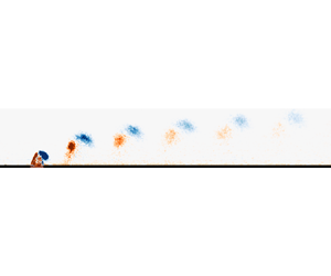
To validate the vortex interaction criterion defined by Johari (Reference Johari2006), we consider cases 22, 23 and 24, which have the same momentum coefficient,  $C_{\mu }=0.73$, but actuation frequencies of 100 Hz, 200 Hz and 400 Hz, respectively (figure 6). At a low actuation frequency $(\,f = 100\ \textrm {Hz},\lambda _i=1.17)$, independent vortical structures can be observed convecting downstream into the far field without any interaction. The substantial tilting of the vortex ring and stretched legs are clear signs of coherent structures. Berk & Ganapathisubramani (Reference Berk and Ganapathisubramani2019) attributed the tilting aspect to the slight self-induced motion of the ring which is in opposition to the incoming flow. These coherent structures are perturbed by an increase in actuation frequency as the vortex interaction index falls below 1.0 ( $f = 200\ \textrm {Hz},\lambda _i=0.57$ and $f = 400\ \textrm {Hz},\lambda _i=0.28$). Under such circumstances, the spatial separation between subsequent pulses abates, leading to vortex interaction. These observations (figure 6b,c) agree with Eroglu & Breidenthal (Reference Eroglu and Breidenthal2001), where the main flow structures consisted of distorted vortex rings which have the stretched leeward portion merged with the windward part of the ring formed during the previous cycle. Additionally, the location at which the interaction occurs shifts further upstream and closer to the orifice exit with a decreasing value of the vortex interaction index.

Figure 6. Plots of the boundary layer subtracted streamwise velocity field,  $\Delta u$, normalised with the free-stream velocity when the jet is at peak blowing, i.e. at phase-locked value of $\phi = 90^{\circ }$, for (a) case 22, (b) case 23 and (c) case 24. These cases have the same aspect ratio and velocity ratio, resulting in the same momentum ratio per cycle of actuation, but differing actuation frequency.
The interaction of vortical structures is also present in the similarity analysis of the phase-locked streamwise velocity field. Keffer & Baines (Reference Keffer and Baines1963) stated that the transverse jet does not achieve self-similarity, as the flow at  $20d$ downstream is still dominated by the twin vortex which prevents any asymptotic tendency towards self-similarity. However, it is clear now that such conclusion emanated from the limited flow field region investigated. In the case of pulsed jets or synthetic jets, the self-similar behaviour of the jet is dependent on the vortex interaction phenomenon. From figure 7, it can be observed that the velocity profile of the jet tends to similarity for cases with vortex interaction. Under such configurations, the coherent structures have already broken down and the flow is analogous to turbulent continuous jets. The interaction of subsequent pulses alters the distribution of vorticity within the structures which undergo disintegration and achieve a quasi-steady jet-like state. These results are consistent with the findings of Amitay et al. (Reference Amitay, Kibens, Parekh and Glezer1999), who observed a reduction in turbulent kinetic energy of the spectrum and the disappearance of any peak corresponding to the passage frequency of coherent structures. The emergence of the spectral band having a $-5/3$ slope was also noted, indicating enhanced dissipation. A similar analysis can be adopted for the interaction of coherent structures in the current study. Interaction and break down of coherent structures lead to a turbulent jet which carries similar properties as a continuous jet in the far field.

Figure 7. Self-similarity analysis for the cases presented in figure 6. (a)  $f = 100\ \textrm {Hz}$, (b) $f = 200\ \textrm {Hz}$ and (c) $f = 400\ \textrm {Hz}$. The velocity deficit $\Delta u$, following subtraction of the unperturbed flow field, is normalised by the maximum velocity-deficit value of the profile ( $\Delta u_{min}$) while $y$,
$y$,  $y_0$ and $y_{1/2}$ represent the wall-normal location, wall-normal location at which the maximum velocity deficit occurs and the jet half-width, respectively.
4. Trajectory scaling
Following categorisation of the experimental data based on the newly derived protocol, nonlinear regression can be applied to the coordinates of the extracted trajectories and the dimensional parameters of the jet. The resulting coefficients and r.m.s. value of the residuals from the fitting procedure (table 3), coupled with prior knowledge from the literature, are utilised to determine the exact form of the non-dimensional numbers relevant in describing the jet trajectory. Subsequently, the physical interpretation and significance of each of the non-dimensional numbers can be established. The exponent of the power law also provides an indication of the jet trajectory. The value of  $n$ in the far field is considerably smaller compared to the near field, implying that the rate of penetration of the jet has diminished in the far field. This already highlights the limitations associated with the use of a single scaling and advocates for delimitation of the flow field. It is important to highlight that the aim is not to find the exact value of the exponents of the non-dimensional groups, but rather to establish the exact form and parameters which are relevant in forming these non-dimensional groups.
Table 3. Fitted coefficients and normalised residuals for  $y/(Dg(\ldots ))=A(x/(Dg(\ldots )))^n$. The 95 % confidence interval limits ( $CI_{95}$) for the fitted parameters are also provided. The coefficients for Berk et al. (Reference Berk, Hutchins, Marusic and Ganapathisubramani2018) presented correspond to data points in the near field with no vortex interaction, obtained by applying the constraints defined in this study.

4.1. Near field with vortex interaction
Based on the coefficients found in table 3, the non-dimensional groups can be formed following (4.1)–4.4, which result in reasonable collapse of the trajectories (figure 8). The jet exit velocity can be coupled with the free-stream velocity to form the velocity ratio. Based on the remaining coefficients, the Strouhal number is observed to depend on the free-stream velocity and a fixed length scale. It is sensible that  $L_1$ takes the form of the momentum thickness, consistent with the notion that the exchange of momentum is important in defining the jet trajectory. The velocity ratio and ratio of length scales ( $l/\theta$) can be rearranged as $C_{\mu }/r$. This quantity represents the ratio of momentum transferred per mass of fluid over a certain area
 \begin{gather} g(\ldots) = \left(\frac{u_j}{u_{\infty}}\right)^{0.85}f^{{-}0.17}l^{1.11}u_{\infty}^{0.17} \theta^{{-}1.28}. \end{gather}
 \begin{gather}g(\ldots) = \left(\frac{u_j}{u_{\infty}}\right)^{0.85}\left(\frac{f \theta}{u_{\infty}}\right)^{{-}0.17}\left(\frac{l}{\theta}\right)^{1.11}. \end{gather}
Rounding off these values results in
 \begin{equation} g(\ldots) = \left(\frac{u_j}{u_{\infty}}\right)\left(\frac{f \theta}{u_{\infty}}\right)^{{-}0.2}\left(\frac{l}{\theta}\right), \end{equation}
which can be rearranged as
 \begin{equation} g(\ldots) =\frac{C_{\mu}}{r}St_1^{{-}0.2}. \end{equation}
Figure 8. (a) Trajectories for all cases listed in table 1 which satisfy vortex interaction, in the near field. (b,c) The trajectories have been scaled by the corresponding  $g(\ldots )$ as defined in (4.4) based on the respective coefficients in table 3. (d) Comparison of the time-averaged trajectories between the experimental data ( $y_{expt}$) and the newly derived model ( $y_{mod}$).
Figures 8(a)–8(d) show the scattered time-averaged jet trajectories pre- and post-scaling with the group of non-dimensional parameters derived in (4.4). The dependence of  $g(\ldots )$ on $C_{\mu }/r$ and a cross-flow-based Strouhal number highlights the importance of momentum transfer between the cross-flow and the jet in determining the near-field trajectory. Such an approach reflects the ideology of Muppidi & Mahesh (Reference Muppidi and Mahesh2005), who emphasised the importance of considering the distribution of momentum when scaling jet trajectories and is further discussed in § 5.
4.2. Far field with vortex interaction
By manipulating the exponents for vortex interaction cases in the far field (4.5)–(4.7), it can be observed that the same non-dimensional numbers as in the near field remain important in collapsing the trajectory
 \begin{gather} g(\ldots) = \left(\frac{u_j}{u_{\infty}}\right)^{0.52}f^{{-}0.2}l^{0.7}u_{\infty}^{0.2} \theta^{{-}0.9}. \end{gather}
 \begin{gather}g(\ldots) = \left(\frac{u_j}{u_{\infty}}\right)^{0.52}\left(\frac{f \theta}{u_{\infty}}\right)^{{-}0.2}\left(\frac{l}{\theta}\right)^{0.7}. \end{gather}
Rounding off these values and rearranging the terms results in
 \begin{equation} g(\ldots) =\sqrt{\frac{C_{\mu}}{r}}St_1^{{-}0.2}\left(\frac{l}{\theta}\right)^{0.2}. \end{equation}
Alternatively, the momentum thickness could be replaced by the orifice slot width to account for the aspect ratio
 \begin{equation} g(\ldots) =\sqrt{\frac{C_{\mu}}{r}}St_1^{{-}0.2}\left(\frac{l}{d}\right)^{0.2}. \end{equation}
 Figures 9(a)–9(d) show the scattered time-averaged jet trajectories pre- and post-scaling with the group of non-dimensional parameters derived in (4.8). The most appropriate parameter to non-dimensionalise the orifice length,  $l$, cannot be established since both the momentum thickness of the boundary layer and the slot width remained unchanged throughout the experiment. However, the inclusion of $d$ agrees with the findings of Van Buren et al. (Reference Van Buren, Beyar, Leong and Amitay2016). The aspect ratio of the orifice is key in reorienting the vorticity in the flow field upon interaction between the coherent structures and bears relevance in the subsequent trajectory followed by the jet. Determining the exact form of this parameter is not within the scope of this study due to the limitation in the dataset. Nonetheless, $g(\ldots )$ reveals that the ratio of momentum per mass of fluid ( $C_{\mu }/r$) is no longer to the leading order. This implies that the bulk of the momentum transfer between the cross-flow and the jet transpires in the near field. The influence of the cross-flow predominates in the far field as the jet convects primarily in the streamwise direction and the flow field echoing characteristics of a quasi-steady flow.

Figure 9. (a) Trajectories for all cases listed in table 1 which satisfy vortex interaction, in the far field. (b,c) The trajectories have been scaled by the corresponding  $g(\ldots )$ as defined in (4.8) based on the respective coefficients in table 3. (d) Comparison of the time-averaged trajectories between the experimental data ( $y_{expt}$) and the newly derived model ( $y_{mod}$).
4.3. Near field with independent vortex rings
If the ejected vortical structures are independent of one another, the near-field trajectories collapse when the non-dimensional groups are formed using (4.9)–(4.11). Formation of the velocity ratio leaves three dimensional parameters ( $f$,
$f$,  $l$ and $u_{\infty }$) with the same exponents, implying that these could be grouped together as the Strouhal number. The exact form of the Strouhal number is found to depend on the length of the orifice aligned with the cross-flow and the free-stream velocity. Although the coefficients/exponents are marginally different, this result is consistent with the findings of Berk et al. (Reference Berk, Hutchins, Marusic and Ganapathisubramani2018), who identified the same non-dimensional numbers. The discrepancy in the values of the exponents is believed to arise from the lack of consideration of the constraints influencing the jet trajectory. Applying the predefined constraints to the dataset from Berk et al. (Reference Berk, Hutchins, Marusic and Ganapathisubramani2018) reveals that $15\,\%$ of the cases in that study incur vortex interaction and $50\,\%$ of the remaining data points are in the near field. Applying nonlinear regression on these points results in the exponents matching the ones in this study (table 3). Any deviations in the values of $A$ and $n$ can be attributed to the number of data points used for the nonlinear regression process
 \begin{gather} g(\ldots) = \left(\frac{u_j}{u_{\infty}}\right)^{1.4}f^{{-}0.4}l^{{-}0.4}u_{\infty}^{0.4}. \end{gather}
 \begin{gather}g(\ldots) = \left(\frac{u_j}{u_{\infty}}\right)^{1.4}\left(\frac{fl}{u_{\infty}}\right)^{{-}0.4}. \end{gather}
Rounding off these values and rearranging the terms result in
 \begin{equation} g(\ldots) =r^{1.4}St_2^{{-}0.4}. \end{equation}
Alternatively, (4.9) can be rearranged such as to include the stroke length,  $L_o$
$L_o$
 \begin{align} g(\ldots) = \left(\frac{u_j}{u_{\infty}}\right)^{1.0}f^{{-}0.4}l^{{-}0.4}u_j^{0.4} = \left(\frac{u_j}{u_{\infty}}\right)^{1.0}\left(\frac{f}{u_j}\right)^{{-}0.4}l^{{-}0.4} = \left(\frac{u_j}{u_{\infty}}\right)^{1.0}\left(\frac{l}{L_o}\right)^{{-}0.4}. \end{align}
Figures 10(a)–10(d) shows the scattered time-averaged jet trajectories pre- and post-scaling with the group of non-dimensional parameters derived in (4.11). The non-dimensional parameters constituting  $g(\ldots )$ indicate that, in the absence of vortex interaction, synthetic jet trajectories in the near field only rely on the initial impulse of the CVP and the spatial separation between subsequent vortical structures, akin to the findings of Berk et al. (Reference Berk, Hutchins, Marusic and Ganapathisubramani2018). The possibility of including the stroke length, important in vortex formation, in (4.12) shows the importance of this parameter in dictating the trajectory of the synthetic jet in the near field. The non-dimensional groups derived in this case show similarities with the scaling derived by Johari (Reference Johari2006) for pulsed jets in cross-flow.

Figure 10. (a) Trajectories for all cases listed in table 1 where there is no vortex interaction in the near field. (b,c) The trajectories have been scaled by the corresponding  $g(\ldots )$ as defined in (4.11) based on the respective coefficients in table 3. (d) Comparison of the time-averaged trajectories between the experimental data ( $y_{expt}$) and the newly derived model ( $y_{mod}$).
4.4. Far field with independent vortex rings
For individual vortical structures in the far field, the nonlinear fitting process reveals that the actuation frequency of the jet is insignificant in determining the trajectory. The velocity ratio and the ratio between the orifice slot length and the momentum thickness of the boundary layer are the pertinent non-dimensional groups which generate the lowest r.m.s. value of the residual. Analysis of the exponents of these parameters indicates that they can be combined together to form the momentum coefficient (1.5)
 \begin{gather} g(\ldots) = \left(\frac{u_j}{u_{\infty}}\right)^{0.58}f^{{-}0.03}l^{0.29}u_{\infty}^{0.03}\theta^{{-}0.32}. \end{gather}
 \begin{gather}g(\ldots) = \left(\frac{u_j}{u_{\infty}}\right)^{0.58}\left(\frac{f \theta}{u_{\infty}}\right)^{{-}0.03}\left(\frac{l}{\theta}\right)^{0.32}. \end{gather}
Rounding off these values and omitting the non-dimensional actuation frequency results in
 \begin{equation} g(\ldots) =C_{\mu}^{0.3}. \end{equation}
Figures 11(a)–11(d) show the scattered time-averaged jet trajectories pre- and post-scaling with the group of non-dimensional parameters derived in (4.15). For this configuration,  $g(\ldots )$ is defined by the momentum coefficient only. It can thus be conjectured that in the absence of any form of interaction, the path followed by independent vortical structures in the far field solely depends on the initial ratio of total momentum between the jet and the cross-flow over one cycle of actuation.

Figure 11. (a) Trajectories for all cases listed in table 1 where there is no vortex interaction in the far field. (b,c) The trajectories have been scaled by the corresponding  $g(\ldots )$ as defined in (4.15) based on the respective coefficients in table 3. (d) Comparison of the time-averaged trajectories between the experimental data ( $y_{expt}$) and the newly derived model ( $y_{mod}$).
5. Discussion
The trajectory of a jet in cross-flow arises since the cross-flow encounters the blockage generated by the jet evolving from the orifice exit. Hence, the cross-flow attempts to oppose and overcome the momentum of the jet by virtue of its own inertial momentum and, in the process, there is a transfer of momentum from the jet to the cross-flow resulting in a momentum deficit and an acceleration of the flow field. This exchange of momentum between the cross-flow and the jet is first used to separate the flow field into two distinct regions: the near field and the far field. Following the derived equation (3.10), it can be observed that the onset of the far field occurs when an appreciable level of momentum transfer has occurred and the flow has reached a certain level of steadiness, as proposed by Van Buren et al. (Reference Van Buren, Beyar, Leong and Amitay2016). The onset of the far field scales with  $\sqrt {C_{\mu }/r}$ while the jet-based Strouhal number is secondary. Following delineation of the flow field and applying Reference JohariJohari's (Reference Johari2006) criterion for vortex interaction, the scaling and relevant non-dimensional parameters for each of the four categories defined in figure 1 were established.
In the event of vortex interaction, the ratio of momentum per mass of fluid between the jet and the cross-flow ( $C_{\mu }/r$) is significant in describing the trajectory and provides an index for the effectiveness of the momentum transfer. The complexity of this process is enhanced because of the additional interactions between the vortical structures themselves, which promote exchange of mass and momentum. The trajectory under such a configuration scales with $r$, consistent with the findings of Broadwell & Breidenthal (Reference Broadwell and Breidenthal1984) and the near-field scaling of Smith & Mungal (Reference Smith and Mungal1998) for steady jets. This can be explained by the breakdown of vortical structures generated by the synthetic jet, which forces the wake to become analogous to that of a steady jet, as demonstrated by the self-similar analysis in the far field (7). The scaling of jet trajectories undergoing vortex interaction in the far field depends on the same non-dimensional parameters as in the near field, although the importance of $C_{\mu }/r$ is reduced. This scaling of $\sqrt {r}$ contrasts with the results of Smith & Mungal (Reference Smith and Mungal1998), who achieved a scaling of $r^2$ in the far field. Such discrepancy arises from the high velocity ratios tested by Smith & Mungal (Reference Smith and Mungal1998). In such cases, the transfer of momentum between the cross-flow and the jet ensues far downstream of the orifice exit and questions the validity of the far-field definition used by Smith & Mungal (Reference Smith and Mungal1998). Based on the concept of momentum transfer and flow steadiness, it can be argued that, since the jets still contained a significant amount of momentum, the far field was not yet reached. In the current study, the low velocity ratios implies that an equilibrium state is already reached in the far field with the jet convecting mostly in the streamwise direction due to the cross-flow and $C_{\mu }/r$ becoming secondary.
Under conditions of vortex interaction, the Strouhal number is expressed in terms of the outer units of the boundary layer and is defined by the momentum thickness and the free-stream velocity. The value of  $\theta /u_{\infty }$ represents a time scale associated with the periodic motion and oscillations within the flow due to interaction of the jet with the cross-flow and interactions between the vortical structures generated by the jet itself. It can be hypothesised that the breakdown of coherent structures generated by the jet as a result of interaction between pulses generates hairpin packets similar to those described by Adrian, Meinhart & Tomkins (Reference Adrian, Meinhart and Tomkins2000). The turbulent boundary layer already contains streaks and the breakdown process results in sinuous and varicose instabilities within the streaks (Skote, Haritonidis & Henningson Reference Skote, Haritonidis and Henningson2002). The value of $\theta /u_{\infty }$ thus represents the time scale of disturbance for such instability mechanisms. Consequently, the Strouhal number depicts the ratio between the time scale of the vortex pair formation by the synthetic jet and the time scale of the disturbance arising from the interaction of the jet with the cross-flow and the pulses themselves. It also describes the effectiveness of adding vortical structures to generate instabilities within the streaks and suppress any bursting event involved in the generation of turbulent skin-friction drag.
When the pulses move independent of one another with no interaction, only the velocity ratio and a Strouhal number based on the orifice length and free-stream velocity are necessary to scale trajectories in the near field. As opposed to vortex interaction cases, accounting for the transfer of momentum between individual vortical structures when they are far apart is inconspicuous. Rather, the impulse of the structure, characterised by the velocity ratio, determines the trajectory followed in the near field. Furthermore, as explained by Berk et al. (Reference Berk, Hutchins, Marusic and Ganapathisubramani2018), the ratio of  $u_{\infty }/f$ gives rise to a length scale representing the spatial separation between successive pulses. If this quantity is comparable to the orifice slot length, $l$, which usually denotes the size of the pulse, then the vortical structures are close together, forming a continuous stream. Assuming negligible interaction, when the value of $fl/u_{\infty }$ is one, the trajectory only depends on $r^{1.4}$. In fact, this is similar to the steady jet scaling derived by Karagozian (Reference Karagozian1986) ( $r^{1.7}$) and falls within the range of values specified by Mahesh (Reference Mahesh2013). Additionally, achieving the same coefficients as Berk et al. (Reference Berk, Hutchins, Marusic and Ganapathisubramani2018) for low Reynolds number flows ( $Re_{\tau } = 1044$) when applying the pre-defined constraints confirms that the scaling of synthetic jet trajectories is not captured through the Reynolds number.
As the individual vortical structures move into the far field, the only parameter having consequential bearing is the ratio between the momentum of the synthetic jet and the momentum contained in the incoming flow, per cycle of actuation. In the far field, a reduction in jet exit velocity and viscous blockage cause the cross-flow to have a commanding influence in convecting the pulses. It follows that the initial momentum of the jet is critical up to the point where the vortex pairs move with the same velocity as the cross-flow. Hence, provided the momentum contained within jets during the blowing cycle is the same, identical trajectories can be achieved in the far field, irrespective of the aspect ratio of the orifice or the velocity ratio. Figure 12 illustrates cases that have the same momentum coefficient but different combinations of  $AR$ and $r$. As expected, the jets in the far field follow the same trajectory. Furthermore, increasing the frequency while maintaining a vortex interaction index greater than 1.0 (case 8) does not alter the jet trajectory as the momentum coefficient is still the same. This result is consistent with the observations of Muppidi & Mahesh (Reference Muppidi and Mahesh2005) who stated that the distribution of momentum in both the jet and the cross-flow should be considered. It also highlights the shortcomings of defining the momentum-flux coefficient with $r^2$ only (independent of the area) when in fact, the distribution of momentum over the area of the orifice exit is more appropriate when scaling the far-field trajectory.

Figure 12. Far-field time-averaged trajectories for cases 7, 8 and 22 which have the same momentum coefficient ( $C_{\mu } = 0.73$) but differing actuation parameters and orifice dimensions.
6. Conclusion
This study investigates the mechanism of scaling synthetic jet trajectories in cross-flow. A synthetic jet is issued in a turbulent boundary layer from orifices with  $AR$ 3, 6 and 12 under contrasting actuation parameters. The aim is to address the disparity observed in previous scaling laws by accounting for constraints associated with the interaction of a jet with an incoming flow. The vortex interaction criterion, defined by Johari (Reference Johari2006), is adopted and complemented with a self-similarity analysis. Existing thresholds used in distinguishing the near field from the far field (Broadwell & Breidenthal Reference Broadwell and Breidenthal1984) were found to be inadequate and a novel expression was defined using the gradient of the trajectory as foundation and nonlinear regression.
Applying these newly defined constraints enables the experimentally acquired dataset to be segregated into four main categories. The scaling for each category is determined via nonlinear regression of the trajectory and dimensional parameters of the jet ( $\overline {u_j}$, $f$,
$f$,  $l$), as this dismisses restrictions arising from using pre-defined non-dimensional groups. Matching the resulting exponents culminates in the relevant non-dimensional groups (figure 13) and the following findings:
(i) The interaction of vortical structures causes a synthetic jet to adopt properties analogous to a steady jet. The near field scales with $r$, consistent with the scaling of steady jets found by Broadwell & Breidenthal (Reference Broadwell and Breidenthal1984) and Smith & Mungal (Reference Smith and Mungal1998). The ratio of momentum per mass flux of the jet and cross-flow emerges as an important parameter in dictating the path followed by a synthetic jet both in the near field and far field.
(ii) When the pulses move independently of one another, the near field scales with
$r^{1.4}St^{-0.4}$. The same non-dimensional parameters and exponents can be recovered from Berk et al. (Reference Berk, Hutchins, Marusic and Ganapathisubramani2018) when applying the constraints defined in this study. Additionally, the exact form of the Strouhal number is observed to consists of the length of the orifice aligned with the flow and the free-stream velocity. As this value approaches 1.0, the vortical structures grow closer together and the trajectory scales with $r^{1.4}$ only, comparable to the scaling found by Karagozian (Reference Karagozian1986) ($r^{1.7}$).(iii) Finally, in the far field, the scaling of independent pulses is observed to be independent of the actuation frequency. Rather, the momentum coefficient is the only parameter important in dictating the jet trajectory. As demonstrated, if the momentum coefficient is kept constant, the same jet trajectory can be achieved for varying combinations of
$AR$ and $r$, provided vortex interaction is not inherent.


This study presents the application of constraints as an important aspect of scaling synthetic jet trajectories in cross-flow and highlights the limitations of using single-scaling laws to describe the complete trajectory. These results constitute an important advancement in fully understanding and predicting the trajectory of synthetic jets in cross-flow and have the potential to enhance and optimise the actuation parameters relevant in applications such as flow control.
Supplementary material
All data supporting this study are openly available from the University of Southampton repository at https://doi.org/10.5258/SOTON/D1679.
Funding
The authors acknowledge the financial support from the Engineering and Physical Sciences Research Council (EPSRC Grant No. EP/L006383/1) and Airbus.
Declaration of interests
The authors report no conflict of interest.


 Open access