


1. Introduction
Bores are ubiquitous in nature. Tidal bores can be found in the upstream of many large river mouths (e.g. the Qiantang River in China). Tsunamis have also been observed in coastal areas in the form of undulating or breaking bores (Shuto Reference Shuto1985; Takahashi & Tomita Reference Takahashi and Tomita2013). It is expected that the length of bore-like tsunamis plays an important role in determining the extent of coastal inundation and overland flows.
Shoaling of bores on a planar beach and bore-induced swash flows have received great attention in the last 60 years. Using the method of characteristics, Whitham (Reference Whitham1958) and Keller, Levine & Whitham (Reference Keller, Levine and Whitham1960) described the evolution of a uniform bore on a planar beach. Their solutions show that the flow velocity behind the bore and the speed of the bore front propagation converge at the still-water shoreline, yielding the shoreline initial velocity. Shen & Meyer (Reference Shen and Meyer1963) further described the shoreline motions. Since their solutions ignore frictional effects, the shoreline motion is driven only by gravity, and the maximum run-up height and its horizontal inundation distance can be calculated as functions of the initial shoreline velocity and beach slope. Peregrine & Williams (Reference Peregrine and Williams2001) extended Shen & Meyer's work and presented solutions for the water depths and flow velocities near the shoreline tip. Hogg, Baldock & Pritchard (Reference Hogg, Baldock and Pritchard2011) studied the swash flows by suddenly releasing a volume of water (dam-break system) on a slope. They applied the hodographic transformation (Carrier & Greenspan Reference Carrier and Greenspan1958) to the nonlinear shallow water equation (NLSWEs). This allowed them to consider the effects of reservoir length on the swash flows and to compare the solutions with those by Shen & Meyer (Reference Shen and Meyer1963) and Peregrine & Williams (Reference Peregrine and Williams2001).
Bore propagation and bore-generated swash flows have been studied in laboratories using different generation systems. Miller (Reference Miller1968) used a piston-type wavemaker to generate bores, and classified them into undulating bores with strength  $F<1.25$ and breaking bores with strength $F>1.55$. In addition, Miller deduced two formulae for the maximum run-up heights as functions of bore height, beach slope and roughness. Baldock, Peiris & Hogg (Reference Baldock, Peiris and Hogg2012) studied the swash flows produced by solitary waves and solitary bores (i.e. ‘single waves that break prior to reaching the still-water shoreline’). Their results show that the duration of the inundation produced by solitary bores is longer than that produced by solitary wave. They also demonstrated that the run-up heights of solitary bores were independent of the wavemaker stroke. Pujara et al. (Reference Pujara, Miller, Park, Baldock and Liu2020) used a piston-type wavemaker to generate three transient waves of elevation with a similar acceleration phase (i.e. the wave front shape), including a solitary wave, successive solitary waves and a short undulating bore. Their experimental data show that the maximum run-up heights are practically the same. On the other hand, they reported that the undulating bore and the successive solitary waves produced larger inundation depths than that produced by the solitary wave. They also generated waves of elevation employing different acceleration phases for the same wavemaker stroke and showed that these waves generated with the same stroke produce similar downrush flows, independent of the wave height. Based on these observations, Pujara et al. (Reference Pujara, Miller, Park, Baldock and Liu2020) further concluded that the wave-integrated volume flux is the parameter with greater influence on the downrush flow.
The most commonly used bore generation mechanism in laboratories is the dam-break system. Stansby, Chegini & Barnes (Reference Stansby, Chegini and Barnes1998) studied the initial stages of dam-break flows and demonstrated that the NLSWE model is adequate in describing the free surface profiles of breaking bores (Stoker Reference Stoker1957; Liggett Reference Liggett1994). Jánosi et al. (Reference Jánosi, Jan, Szabó and Tél2004) provided measurements of the bore front propagation for two breaking bores of different strengths. These results were later used in Goater & Hogg (Reference Goater and Hogg2011) to validate the bore front propagation modelling using the hodograph transformation of the NLSWEs. Excellent agreement was observed for both non-decaying bores and decaying bores. More recently, Lin et al. (Reference Lin, Kao, Yuan, Raikar, Hsieh, Chuang, Syu and Pan2020a,Reference Lin, Kao, Yuan, Raikar, Wong, Yang and Yangb) studied undulating bores on a horizontal bed with different reservoir lengths and they also measured the velocity fields. Yeh, Ghazali & Marton (Reference Yeh, Ghazali and Marton1989) used a 2.97 m long reservoir to generate undulating and breaking bores on a  $7.5^{\circ }$ smooth Plexiglas beach. They found that the shoreline motion decelerates faster than the shallow water wave prediction, and concluded that the maximum run-up height can be predicted by Shen & Meyer's theory if a smaller initial shoreline velocity is used. Other researchers have also investigated different characteristics of swash flows. Barnes et al. (Reference Barnes, O'Donoghue, Alsina and Baldock2009), O'Donoghue, Pokrajac & Hondebrink (Reference O'Donoghue, Pokrajac and Hondebrink2010) and Kikkert et al. (Reference Kikkert, O'Donoghue, Pokrajac and Dodd2012) used a 1 m long reservoir to study bottom shear stress, flow depth and velocity produced by short breaking bores on a 1 : 10 slope with different roughness. Dai et al. (Reference Dai, Kikkert, Chen and Pokrajac2017) employed a similar set-up to study the entrained air in breaking bores and concluded that the effect of air bubbles on swash flows is small, supporting the assumption that the swash flows can be modelled as a single phase fluid. Lin et al. (Reference Lin, Kao, Wong, Shao, Hu, Yuan and Raikar2019) generated undulating bores to study the swash flows on a 1 : 20 slope using a 3.76 m long reservoir. Hogg et al. (Reference Hogg, Baldock and Pritchard2011) installed a dam-break system on a tilting tank to study bore-induced overtopping volumes. In their experiments three slopes (1 : 10, 1 : 20 and 1 : 30) were used, and the reservoir length was varied between 1 and 2 m. Their dam-break system, being on the slope, is different from the traditional set-ups on a horizontal bottom; their generated bores are also different. Nevertheless, they showed that the length of reservoir has an influence on the generated swash flows.
Numerical simulations have also been employed to study bore generated swash flows. Hibberd & Peregrine (Reference Hibberd and Peregrine1979) adopted a finite difference method to solve the NLSWEs for bores climbing on a planar beach. At beach toe, the flow depth and velocity were prescribed to generate uniform bores. Their simulations showed that a flooding plateau (constant depth) appeared during which the flow velocities were close to zero. Using a similar numerical method, Guard & Baldock (Reference Guard and Baldock2007) studied the swash flows produced by non-uniform bores. The bore characteristics were introduced at the initial shoreline, in terms of the Riemann invariant  $\alpha$ (to be defined in § 2). Their results point out that the shoreline motion, and therefore the maximum run-up, follows a parabola, which only depends on the characteristics of the bore front. On the other hand, the inundation depths vary for different boundary flow conditions. In contrast to Hibberd & Peregrine, Guard & Baldock (Reference Guard and Baldock2007) did not find the formation of a flooding plateau. Finally, Guard & Baldock compared their numerical results of the swash flow depths with laboratory data, showing a good agreement for a specific boundary condition. Chan & Liu (Reference Chan and Liu2012) solved the NLSWEs with a Lagrangian numerical method and investigated the evolution and run-up of non-breaking long waves on a plane beach, which is connected to a constant depth region. They showed that the maximum run-up height is a function of the front profile of the leading tsunami wave. Briganti et al. (Reference Briganti, Torres-Freyermuth, Baldock, Brocchini, Dodd, Hsu, Jiang, Kim, Pintado-Patiño and Postacchini2016) provided a comprehensive review of the numerical modelling of swash zone processes and used the experiments of Kikkert et al. (Reference Kikkert, O'Donoghue, Pokrajac and Dodd2012) as a benchmark. They concluded that the depth-averaged wave models can accurately reproduce free surface elevations and depth-averaged velocity measurements. On the other hand, the Reynolds-averaged Navier–Stokes and large eddy simulation models can produce more detailed predictions of turbulence components of the flow for a significant extra computational cost (e.g. Shigematsu, Liu & Oda Reference Shigematsu, Liu and Oda2004; Zhang & Liu Reference Zhang and Liu2008).
The literature review suggests that bore-induced swash flows are strongly influenced by the bore strength and bore length at the beach toe. However, the dependency has not been determined quantitatively. In this study we seek to fill this knowledge gap. The objective is to find the correlations between the swash flow characteristics (inundation depth, run-up height and flooding duration) with the bore characteristics (bore strength and bore length) at the beach toe and the beach slope. To accomplish this, we first conduct laboratory experiments using a dam-break system with variable reservoir length. A 1 : 10 beach made out of glass is installed for generating swash flows. Bores are generated with different reservoir lengths and different bore strengths, which are determined by the ratio of water depths inside and outside of the reservoir. Using the laboratory measurements, the swash flow characteristics are related to the bore strength at the dam-break gate and the reservoir length. The analytical relations between the bore characteristics at the dam-break gate and those at the beach toe are obtained by using the method of characteristics. These relations can be used to design a dam-break set-up to generate a desirable bore with targeted bore length and strength at beach toe. Since only a limited number of laboratory experiments can be conducted (e.g. only one slope), and physical flow variables can only be measured at discrete locations, the numerical model SWASH (Zijlema, Stelling & Smit Reference Zijlema, Stelling and Smit2011) is employed to generate additional data to cover a wider range of physical parameters. The numerical model is first validated against the laboratory data. Finally, predictive formulae relating the bore characteristics at the beach toe with the corresponding swash characteristics are deduced based on the numerical simulation results.
This paper is structured as follows. In the next section several bore features are defined using the nonlinear shallow water theory and the method of characteristics. In § 3, a dam-break system and experimental conditions are described, and the laboratory results for bores with different strengths and lengths are presented. In § 4, dam-break bores and their evolution in a constant depth are studied and analytical relations are presented. In § 5, the numerical model for simulating dam-break bore experiments is introduced. A parametric analysis is carried out to study the influence of the bore characteristics (bore strength and bore length) at the beach toe and beach slope on the swash flow characteristics (inundation depth, run-up and flooding duration). Based on the numerical results, predictive relations are deduced. Finally, in § 6, concluding remarks are provided.
2. General definitions of bores
Figure 1 shows sketches of undulating and breaking bores of finite length with a uniform depth  $h_b$ and fluid velocity $u_b$ throughout its plateau. The bore front moves with a constant velocity, $U_b$, propagating into the undisturbed water depth, $h_0$, on a horizontal bed. At the end of the plateau a bore tail is formed, where the water depth and fluid velocity decrease. The distance between the bore front and the beginning of the bore tail defines the bore length $L_b$.

Figure 1. Definition sketch for a bore of limited length propagating on a horizontal bed. (a) Undulating bore and (b) breaking bore.
The formation of bores and their propagation can be described by the NLSWEs (e.g. Peregrine Reference Peregrine1972) in terms of the depth-averaged horizontal velocity,  $u(x,t)$, and the free surface displacement, $\eta (x,t)$. The NLSWEs can also be written in the form of characteristics equations (e.g. Liggett Reference Liggett1994), in which two (positive and negative) characteristics are defined as ${\textrm {d} x}/\textrm {d}t = u+ c$ and ${\textrm {d} x}/\textrm {d}t = u- c$, respectively, where $c = \sqrt { g( h +\eta ) }$ is the local long-wave celerity with $h$ being the water depth and $g$ being the gravitational acceleration. The Riemann invariants, $\alpha =u+2c$ and $\beta =u-2c$, remain constant on each positive and negative characteristics, respectively.
Defining the bore strength as
 \begin{equation} F=\frac{U_b}{c_0}, \end{equation}
where  $c_0=\sqrt {gh_0}$ is the long-wave celerity in front of the bore and $F > 1$ represents a positive surging bore, and invoking the conservation of mass and momentum in the vicinity of bore front, the bore strength can be related to $u_b$, $h_b$ and $h_0$ as (Stoker Reference Stoker1957; Liggett Reference Liggett1994)
 \begin{gather} \frac{u_b}{c_0}=F\frac{\sqrt{1+8F^2}-3}{\sqrt{1+8F^2}-1}, \end{gather}
 \begin{gather}\frac{h_b}{h_0}=\left(\frac{c_b}{c_0}\right)^2=\frac{1}{2}({\sqrt{1+8F^2}-1}), \end{gather}
where  $c_b=\sqrt {gh_b}$ is the bore celerity. Any infinitesimal disturbance initiated on the bore plateau propagates forward with the speed of $u_b+c_b$ and backward with $u_b-c_b$. For $F>1$, the forward propagating disturbance will eventuality catch up with the bore front, since $(u_b+c_b)>U_b$ from (2.2) and (2.3). Therefore, the bore length ( $L_b$) decreases as the bore propagates. Once the bore length is reduced to zero, the flow momentum behind the bore front starts to decrease and the bore cannot sustain its initial strength. At this moment, the bore becomes a decaying bore. Studying the behaviour of decaying bores is beyond the scope of this paper; only the non-decaying bores are analysed herein.
The theoretical description of bore generation mechanisms using a dam-break system can be found in the literature, mostly based on the NLSWEs (Liggett Reference Liggett1994). Figure 2 shows a sketch of the initial set-up in a dam-break system. Once the gate is instantaneously lifted, a bore is formed (see figure 2b). According to the method of characteristics, positive characteristics departing from the reservoir water ( $u=0$) have an $\alpha$ value: $\alpha =u+2c=2c_1$, where $c_1=\sqrt {gh_1}$ is the long-wave celerity for the undisturbed water in the reservoir. The ratio between the water depths on both sides of the gate can then be calculated as a function of the bore strength (Liggett Reference Liggett1994),
 \begin{equation} \frac{c_1}{c_0}=\frac{1}{2}\frac{u_b}{c_0}+\frac{c_b}{c_0}, \end{equation}
in which the terms on the right-hand side depend only on  $F$, according to (2.2) and (2.3). Thus, in designing a laboratory experiment, the water depth, $h_0$ (or $c_0$), can be fixed first. For a desirable bore strength, $F=F_{in}$, the necessary water depth in the reservoir, $h_1$ (or $c_1$) is determined from (2.4). This will be further discussed in the following section.

Figure 2. (a) Initial conditions of a dam-break system. (b) Representation of the generated bore.
The length of the reservoir will affect the length of the bore. Applying the hodograph transformation to the NLSWEs (Carrier & Greenspan Reference Carrier and Greenspan1958; Carrier, Wu & Yeh Reference Carrier, Wu and Yeh2003), Hogg (Reference Hogg2006) and Goater & Hogg (Reference Goater and Hogg2011) analysed the influence of the reservoir length in the bores generated. Their findings will be further discussed in § 4 and Appendix A.
3. Laboratory experiments
Physical experiments have been carried out in a flume in the hydraulic laboratory at the National University of Singapore (NUS). The flume is 36 m long, 0.9 m high and 0.9 m wide. At one end of the flume a 6 m long glass beach (1 : 10 slope) is installed. The distance from the dam-break gate to the beach toe is  $L_f= 11.1$ m (see figure 3). The small gaps between the edges of the gate and the flume walls and floor are sealed with a customized rubber profile to make them watertight when the gate is at rest in the water. The gate is controlled by a pneumatic system and its movement is triggered by a digital signal. The averaged lifting time for the entire gate stroke (0.9 m) is 0.987 s with a standard deviation of 0.112 s. The vertical position of the gate is tracked using two reed switches, allowing synchronization between the gate and the data acquisition. In addition, a 0.6 m high waterproof coated plywood wall is positioned behind the gate to create a reservoir. Four reservoir lengths have been used in this study, i.e. $L_r=2$, 4, 8 and $17.6$ m, respectively. For each set-up, experiments are repeated three times. All the measured data from each run are analysed.

Figure 3. Dam-break experimental set-up in the NUS hydraulic laboratory (not to scale).
As shown in figure 3, four capacitance gauges (CG) are installed in the constant depth area; the first gauge is always located inside the reservoir and the last one at the beach toe. In addition, three ultrasound sensors (US) are installed on the beach to measure the free surface elevations without disturbing the swash flows. The second US for cases of  $L_r= 2$, 4 and 8 m and the first US for the case of $L_r=17.6$ m are located at the still-water shoreline location. The sensor locations are summarized in table 1. The data sampling rate for both types of sensors is 200 Hz. Finally, the run-up on the beach is recorded with a full high-definition camera placed above the beach. The recording speed is 100 frames per second. The frames with highest shorelines are identified and digitized to quantify the maximum run-up heights.
Table 1. Sensor locations in metres with the origin at the gate.

The constant water depth is fixed at  $h_0=0.1$ m for all experiments. The water depth in the reservoir ( $h_1$) is calculated for a target bore strength, using (2.2), (2.3) and (2.4). A summary of the water depth ratios is given in table 2.
Table 2. Input water depth ratios ( $h_1/h_0$) based on the target input bore strength ( $F_{in}$); $h_0 = 0.1$ m.
3.1. Experimental observations
For illustration purposes, the time histories of free surface elevation at CG2 for the undulating bore case ( $F_{in}=1.2$), the undulating–breaking bore case ( $F_{in}=1.5$) and the breaking bore case (
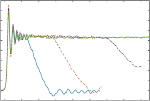
 $F_{in}=1.9$) are plotted in figures 4, 5 and 6, respectively. In each figure, measurements for four different reservoir lengths are included. The free surface data are synchronized at their arrival times at CG2, and for clarity the records are truncated without showing the reflections from the beach.

Figure 4. Time histories of dimensionless free surface elevations at CG2 for undulating bore with strength of  $F_{in}=1.2$. Two views are presented: while the zoomed-out view is shown in panel (a), the details of the bore front are shown in panel (b). Results: $L_r/h_0=20$ (blue line); $L_r/h_0=40$ (orange line); $L_r/h_0=80$ (purple line); $L_r/h_0=176$ (green line). Squares represent the arrival of bore front, triangles the beginning of tail and circles the first measurement with bore height equal to or larger than the bore height at the beginning of the bore tail.

Figure 5. Time histories of dimensionless free surface elevations at CG2 for undulating bore with strength of  $F_{in}=1.5$. Two views are presented: while the zoomed out view is shown in panel (a), the details of the bore front are shown in panel (b). Results: $L_r/h_0=20$ (blue line); $L_r/h_0=40$ (orange line); $L_r/h_0=80$ (purple line); $L_r/h_0=176$ (green line). Squares represent the arrival of bore front, triangles the beginning of tail and circles the first measurement with bore height equal to or larger than the bore height at the beginning of the bore tail.

Figure 6. Time histories of dimensionless free surface elevations at CG2 for undulating bore with strength of  $F_{in}=1.9$. Two views are presented: while the zoomed out view is shown in panel (a), the details of the bore front are shown in panel (b). Results: $L_r/h_0=20$ (blue line); $L_r/h_0=40$ (orange line); $L_r/h_0=80$ (purple line); $L_r/h_0=176$ (green line). Squares represent the arrival of bore front, triangles the beginning of tail and circles the first measurement with bore height equal to or larger than the bore height at the beginning of the bore tail.
For the cases with  $F_{in}=1.2$, undulating bores are generated. In the stronger bore strength cases ( $F_{in} = 1.5$ and 1.9), bores are breaking with steeper bore fronts. In figure 4 ( $F_{in}=1.2$), for different reservoir lengths the undulating bore lasts a different duration before the bore height starts to decrease, forming a bore tail. As expected, the longest bore is produced by the longest reservoir $L_r/h_0=176$, which does not show the bore tail because the wave reflection from the slope reaches this gauge before the bore height starts to decrease. Finally, the bores generated with the same reservoir length become shorter for larger bore strengths (see figures 5 and 6).
As shown in figures 4, 5 and 6, the arrival times of the bore front (denoted by squares) and the beginning of the bore tail (triangles) have been identified for all cases. The arrival time of the bore front is defined as the moment when the dimensionless free surface elevation becomes larger than 0.02. The same definition is applied to the measurements at CG2, CG3 and CG4.
The method for identifying the beginning of the bore tail is briefly summarized here (more details can be found in the supplementary materials available at https://doi.org/10.1017/jfm.2021.98). For each time record, a histogram of the normalized free surface elevation,  $\eta /\eta _{max}$, is constructed. The bin size used in the histogram is 0.05 with 50 % overlapping. The bin that has the highest percentage of occurrence represents the bore plateau and the last measurement (in time) in this bin is designated as the beginning of the bore tail. The bore height ( $h_b$) is calculated as the average of the bore heights between the following two instants. The first moment is when the first height measurement is equal to or larger than the height at the beginning of the tail (circles in figures 4, 5 and 6), and the second instant is the beginning of the bore tail. The bore period is defined as the time interval between the bore front arrival and the beginning of the bore tail. The bore periods are only recorded for the cases in which the beginning of the bore tail reaches the gauge before the reflection does. The bore heights and periods have been measured at CG2 and CG3.
The strength of a bore travelling from CG2 to CG3 (in the constant depth region) can be approximately estimated by using the bore front arrival times at the gauges and the distance between the gauges as
 \begin{equation} F_{23}=\frac{x_{3}-x_{2}}{(t_{3}-t_{2})\sqrt{gh_0}}, \end{equation}
where  $x_{3}$ and $x_{2}$ are the locations of the gauges (see table 1) and $t_{3}$ and $t_{2}$ are the arrival times estimated at the respective gauges. The strength of the bore travelling from CG3 to CG4 is calculated in a similar way and is denoted as $F_{toe}$, which is used to define the bore strength at the beach toe. In figure 7, $F_{23}$ and $F_{toe}$ are plotted versus the input bore strength, $F_{in}$, estimated at the gate of the dam-break system. All the data obtained for the experiments listed in table 2 have been processed and shown in the same figure. The measured bore strengths fit closely with the bore strengths predicted by the NLSWEs (i.e. (2.1), (2.2), (2.3) and (2.4)). The bore height measurements at CG2 and CG3 are plotted against the measured bore strength $F_{23}$ in figure 8. The measured bore heights agree well with the theoretical predictions based on NLSWEs (2.3). The data scattering observed in the bore heights is larger than that observed in the bore strengths, especially for the strongest cases. As seen in figures 5 and 6, undulations are observed riding the bore plateau even for breaking bores. In addition, the process used to identify the beginning of the bore tail may include a portion of the bore tail within the range of the histogram's window size. The influence of these two phenomena in the calculation of the average bore heights increases for shorter bores. The $R^2$ values between all the laboratory measurements and the NLSWEs predictions (plotted with dashed lines in figures 7 and 8) are $R^2=0.990$ for the bore strength and $R^2=0.981$ for the bore height. These comparisons show an excellent agreement between laboratory measurements and theoretical predictions and further prove that the NLSWE theory adequately describes the bore propagation in constant depth and both the bore strength and bore height are uniform in the constant depth region.

Figure 7. Measured bore strengths between CG2 and CG3 (a), and between CG3 and CG4 (b), for different reservoir length and bore strength. The dashed line represents the theoretical bore strength.

Figure 8. Measured bore heights at CG2 (a), and at CG3 (b) for different reservoir length and measured bore strengths. The dashed line represents the theoretical bore height correspondent to a given bore strength (2.3).
The time histories of the free surface elevations at the still-water shoreline for undulating bores ( $F_{in}=1.2$), undulating–breaking bores ( $F_{in}=1.5$) and breaking bores ( $F_{in}=1.9$) are plotted in figures 9, 10 and 11, respectively. The free surface measurements have been synchronized at their arrival time at the still-water shoreline for comparison purposes. Because of the steep free surface slope in undulating bores, signal dropouts can be seen in the US records.

Figure 9. Time histories of dimensionless free surface elevations at the still-water shoreline are shown for undulating bore with strength of  $F_{in}=1.2$. (a) The time histories for a longer period of times are shown, while the details of the bore front are shown in panel (b). Results: $L_r/h_0=20$ (blue line); $L_r/h_0=40$ (orange line); $L_r/h_0=80$ (purple line); $L_r/h_0=176$ (green line). Circles represent the maximum free surface height ( $I/h_0$); diamonds represent the beginning of the flooding plateau and triangles the end of the flooding plateau.

Figure 10. Time histories of dimensionless free surface elevations at the still-water shoreline are shown for undulating bore with strength of  $F_{in}=1.5$. (a) The time histories for a longer period of times are shown, while the details of the bore front are shown in panel (b). Results: $L_r/h_0=20$ (blue line); $L_r/h_0=40$ (orange line); $L_r/h_0=80$ (purple line); $L_r/h_0=176$ (green line). Circles represent the maximum free surface height ( $I/h_0$); diamonds represent the beginning of the flooding plateau and triangles the end of the flooding plateau.

Figure 11. Time histories of dimensionless free surface elevations at the still-water shoreline are shown for undulating bore with strength of  $F_{in}=1.9$. (a) The time histories for a longer period of times are shown, while the details of the bore front are shown in panel (b). Results: $L_r/h_0=20$ (blue line); $L_r/h_0=40$ (orange line); $L_r/h_0=80$ (purple line); $L_r/h_0=176$ (green line). Circles represent the maximum free surface height ( $I/h_0$); diamonds represent the beginning of the flooding plateau and triangles the end of the flooding plateau.
At the time the bores reach the shoreline, the water depths rise quickly and the bore fronts have very similar shape for all input bore strengths. For undulating bores the water depths continue to increase in an oscillatory manner until the maximum inundation depth is achieved (figure 9). For undulating–breaking and breaking bores the water depths increase with a more linear trend (figures 10 and 11).
The maximum inundation depths,  $I/h_0$, are denoted by circles in figures 9, 10 and 11, which depend strongly on the reservoir length for stronger bores. For the longest reservoir case ( $L_r/h_0=176$), a plateau is formed for all different bore strength. A flooding plateau also appears for $L_r/h_0=80$ with $F_{in}=1.2$ and 1.5, and for $L_r/h_0=40$ with $F_{in}=1.2$ (figures 9 and 10). During the flooding plateau the water is locally quiescent. It is observed that cases with different reservoir length generate flooding plateaus of different duration.
The beginning and the end of the flooding plateau at the still-water shoreline are identified with a methodology similar to the identification of the beginning of the bore tail discussed above. A histogram of the normalized free surface elevation,  $\eta /\eta _{max}$, is first constructed. The bin size is 0.05 with 50 % overlapping. The bin with the maximum number of measurements represents the flooding plateau. The beginning and the end of the flooding plateau are identified as the first and last measurement points (in time), after the maximum inundation depth, within this bin. The duration of the flooding plateau is calculated as the time interval between the beginning and the end of the flooding plateau. More details on the flooding plateau analysis are provided in the supplementary materials.
In figure 12 the maximum inundation depths measured at the still-water shoreline are plotted versus  $F_{toe}$, which contains all the experimental data listed in table 2. The maximum inundation depths for the long reservoir cases, $L_r/h_0=80$ and $176$, follow the same trend for the entire range of bore strengths. On the other hand, for shorter reservoirs the maximum inundation depths still follow the same trend for a range of small bore strengths, however, as the bore strength exceeds a certain value, the inundation depth takes on a different trend with a milder slope. The shorter the reservoir length is, the sooner the maximum inundation depths drift from the original trend. Similarly, the maximum run-up heights for all the experiments are plotted for different $F_{toe}$ in figure 13. The maximum run-up height is not affected by the reservoir length; for the same bore strength, the maximum run-up heights are practically identical. The maximum run-up predicted by the Shen & Meyer (Reference Shen and Meyer1963) solution is calculated by employing the shoreline velocity of Keller et al. (Reference Keller, Levine and Whitham1960). Laboratory maximum run-up heights are, on average, 60 $\%$ of the predicted solution by Shen & Meyer for $F_{toe}>1.23$.

Figure 12. Dimensionless inundation depths at the still-water shoreline,  $I/h_0$, in terms of the bore strength measured at the beach toe, $F_{toe}$, and the reservoir length, $L_r/h_0$. The black solid line represents the predictive equation (5.2) and the dashed coloured lines equation (5.1), in which $L_b$ is calculated using (4.5).

Figure 13. Dimensionless maximum run-up,  $R/h_0$, in terms of the bore strength at the beach toe, $F_{toe}$ and the reservoir length, $L_r/h_0$. The solid black line represents the predictive solution (5.4) and the dashed line represents Shen & Meyer (Reference Shen and Meyer1963) run-up solution.
From figure 12, it is clear that different reservoir lengths produce different inundation depths for the same bore strength at the beach toe. It is important to recall that the laboratory experiments were performed for a fixed slope ( $s=1/10$) and a fixed distance between the beach toe and the location of the dam-break gate (i.e. $L_f=11.1$ m in figure 3). Since bores evolve as they propagate in the constant depth, for the same dam-break system set-up, the distance $L_f$ plays an important role in determining the bore characteristics at the beach toe, and thus, the resulting run-up heights and inundation depths at the still-water shoreline.
In figure 14 the duration of the flooding plateau at the still-water shoreline,  $T_f$, which will be called flooding duration hereafter, are plotted versus $F_{toe}$. Only the flooding duration for cases which are long enough to generate a flooding plateau are shown (more details are provided in § 5.2). For $L_r/h_0=176$, flooding plateaus appear for the entire range of bore strengths, and the duration decreases as the bore strength increases. For $L_r/h_0=40$ and 80, flooding plateaus appear for $F_{toe}\leqslant 1.3$ and 1.6, respectively. However, the plateau disappears for stronger bores (see figures 9 to 11). In general, the flooding duration increases when the reservoir length increases, with the bore strength being fixed. For $L_r/h_0=20$ a flooding plateau only appears for $F_{toe}\approx 1.1$, with a duration close to zero.


It is more useful to express the maximum inundation depth at the still-water shoreline,  $I$, the maximum run-up height, $R$, and the flooding duration, $T_f$, in terms of the bore characteristics at the beach toe, i.e.
 \begin{gather} \frac{I}{h_0}=f_1\left( F_{toe},\frac{sL_b}{h_0},s \right), \end{gather}
 \begin{gather}\frac{R}{h_0}=f_2\left( F_{toe}, \frac{sL_b}{h_0}, s \right), \end{gather}
 \begin{gather}sT_f\sqrt{\frac{g}{h_0}}=f_3\left( F_{toe},\frac{sL_b}{h_0},s \right), \end{gather}
where  $f_i$ ( $i =1, 2, 3$) are functions to be determined, $L_b$ denotes the bore length at the beach toe and its dimensionless form is normalized by the horizontal distance from the beach toe to the still-water shoreline, $h_0/s$. In so doing, the swash flow characteristics are independent of the bore generation mechanism. However, since the dam-break system is used in the experiments to generate the incoming bores, the bore characteristics at the beach toe must be first related to the dam-break system parameters, i.e.
 \begin{equation} \frac{L_b}{h_0}=f_4\left(F_{in},\frac{L_r}{h_0}, \frac{L_f}{h_0} \right), \end{equation}
in which the input bore strength,  $F_{in}$, is a function of $h_1$ and $h_0$ as discussed in § 2. It is recalled that, for the non-decaying bores ( $L_b>0$) the bore strength remains constant in the constant depth region (i.e. $F_{in}=F_{toe}$, see figure 7).
In the following section the method of characteristics is first used to establish (3.5). In § 5 numerical simulations of dam-break generated swash flows are performed for a large range of physical parameters and the results are employed to establish the relationships in the form of (3.2), (3.3) and (3.4). The experimental data are used to check the accuracy of the numerical results. Combining the information obtained in §§ 4 and 5 leads to the predictions of inundation depth, maximum run-up height and flooding duration produced by a given dam-break set-up. The information can also be used to design a dam-break system to produce a target flooding scenario.
4. Bore period and bore length analysis
As shown in Hogg (Reference Hogg2006) and Goater & Hogg (Reference Goater and Hogg2011), the bore period can be estimated by the method of characteristics and the bore relations presented in § 2.
In this paper we define the bore period ( $T_{bt}$) as the time interval between the time when the bore front reaches a certain location ( $t_{arr}$) and the time when the beginning of the tail of the bore crosses the same location ( $t_{end}$),
 \begin{equation} T_{bt}=t_{end}-t_{arr}, \end{equation}
which is measurable in the experiments (see figures 4, 5 and 6). As shown in Appendix A, the bore period at a given location,  $x_t$, can be calculated by (see (A5))
 \begin{equation} T_{bt}=L_r\left(\frac{8\sqrt{c_1}}{(2c_1-u_b+2c_b)^{3/2}}\right)\left(1-\frac{u_b-c_b}{u_b+c_b}\right)+x_t\left(\frac{U_b-u_b-c_b}{U_b(u_b+c_b)}\right), \end{equation}
where  $U_b/c_0$, $u_b/c_0$, $c_b/c_0$ and $c_1/c_0$ can all be expressed in terms of $F_{in}$, using (2.1), (2.2), (2.3) and (2.4), respectively.
To check the accuracy of (4.2), the experimental data at gauges CG2 and CG3 are used for comparison (figure 15). As indicated in the figure, the calculated bore periods are very accurate at CG2. However, at CG3 the experimental data is more scattered for  $Lr/h_0 = 20$, especially for $1.3 < F_{23} < 1.4$, which correspond to the shortest undulating–breaking bores. In these cases, undulations appear on the bore plateau and at the bore tail. While the methodology used to measure the bore duration is generally robust, these undulations affect the accuracy of the bore duration measurements. The uncertainties become larger for shorter bores. The $R^2$ value between the bore periods measured in the laboratory and the predicted by (4.2) is $R^2=0.979$.

Figure 15. The bore periods measured at CG2 on panel (a), and CG3 on panel (b), for different reservoir lengths. Markers represent experimental data. Lines are calculated using (4.2) by substituting the input parameters ( $F_{in}, L_r$) at CG2 and CG3, where $x_t$ is the location of the respective CG (see table 1).
The evolution of the bore length can also be estimated using the method of characteristics and the bore relations. As shown in Appendix A, the initial bore length generated at the dam-break gate,  $L_{b0}$, can be calculated as (see (A7) and (A8))
 \begin{equation} \frac{L_{b0}}{h_0}=K\frac{L_r}{h_0}, \end{equation}
with
 \begin{equation} K=\frac{8\sqrt{c_1}c_0}{(2c_1-u_b+2c_b)^{3/2}}\left(F_{in}-\frac{(u_b-c_b)}{c_0}\right). \end{equation}
The equations above provide an analytical expression for estimating the initial bore length as a function of the reservoir length ( $L_r$) and the bore strength. For $1 < F < 2$, $K$ is approximately 2, suggesting that the initial bore length is roughly twice the reservoir length.
As the bore propagates away from the gate, the bore length decreases since the end of the bore plateau propagates faster than the bore front does. As shown in Appendix A, the bore length reaching the beach toe can be calculated as (see (A10))
 \begin{equation} L_{b}=L_r\left(\frac{16\sqrt{c_1}c_b}{(2c_1-u_b+2c_b)^{3/2}}\right)-\frac{L_f}{F_{in}}\left(\frac{u_b+c_b}{c_0}-F_{in}\right). \end{equation}
We reiterate that  $u_b/c_0$, $c_b/c_0$ and $c_1/c_0$ can be expressed in terms of $F_{in}$ as given in (2.2), (2.3) and (2.4), respectively. Equation (4.5) can also be used to determine the reservoir length, $L_r$, required to generate a bore that will reach the beach toe with a targeted bore length and bore strength.
Up to this point, we can convert the experimental conditions to the bore length and bore strength at the beach toe. Thus, the inundation depth, run-up height and flooding period can be predicted according to the incoming bore characteristics at the beach toe and beach slope. However, the range of physical parameters used in the laboratory experiments is rather limited. In order to provide additional swash flow data with a wider range of bore length and strength at beach toe and beach slope, numerical simulations are performed. To be consistent with the laboratory experiment, (4.5) is used to set up the dam-break system in the numerical simulations. In addition, the bore lengths measured in the numerical simulations are used to evaluate the accuracy of (4.5).
5. Numerical simulations
The numerical model SWASH is employed in this study. The model solves the NLSWEs with the non-hydrostatic pressure to describe depth-averaged free surface flows. A momentum conservative shock capturing scheme, the hydrostatic front approximation (known as HFA) of Smit, Zijlema & Stelling (Reference Smit, Zijlema and Stelling2013), is used to model wave breaking. The hydrostatic front approximation defines wave breaking when the time rate of change of the free surface ( $\partial \eta / \partial t /\sqrt {gh}$) exceeds a certain value $\delta$. Smit et al. empirically determined $\delta =0.6$, based on the experiments of Ting & Kirby (Reference Ting and Kirby1994). Once wave breaking is triggered, the non-hydrostatic pressure term is disabled, and the bore-like breaking process takes control. The model discretizes the numerical domain into a fixed number of vertical layers in order to improve the frequency dispersion. Because this study focuses on long bores, only a single layer is used in the vertical direction.
All the numerical simulations presented herein mimic the physical dam-break experiments. However, the spanwise direction is ignored and therefore the numerical simulations become one-dimensional. The input parameters are: reservoir length ( $L_r$); distance from the dam-break gate to the beach toe ( $L_f$); slope ( $s$); and water depths upstream ( $h_1$) and downstream ( $h_0$) of the gate, respectively. All meshes have a constant grid size in the constant depth region. This grid size is reduced linearly by one tenth from the beach toe until the still-water shoreline, from there it remains constant until the top of the slope. The maximum Courant number (Courant–Friedrichs–Lewy condition) is fixed for all simulations at 0.5.
The model has been calibrated and validated using the laboratory measurements at the beach toe and the still-water shoreline for the case  $L_r/h_0=80$ with input bore strengths of $F_{in}=1.1$, $1.2$ and $1.5$. All the validation results are reported in the supplementary materials. Based on the model validation, the grid size is set to be 0.02 m and the breaking wave condition at $\delta = 0.8$. In addition, the comparison between laboratory measurements and numerical results points out the lifting speed of the dam-break gate can be considered instantaneous for the scope of this study. Comparisons between the laboratory experiments and numerical results for the maximum inundation depth at the still-water shoreline, the maximum run-up heights and the flooding duration are reported in Appendix B.
5.1. Parametric analysis
To study the influence of different parameters on the swash process, i.e. (3.2), (3.3) and (3.4), numerical simulations have been conducted for a range of target bore strengths ( $F_{in}$) and bore lengths at the beach toe ( $L_b$) and slopes ( $s$) with a fixed water depth ( $h_0$). The range of these parameters is summarized in table 3. The incremental changes for $F_{in}$ and $sL_b/h_0$ are 0.05 and 2.5, respectively. A total of 2400 numerical simulations have been carried out.
Table 3. Summary of the numerical simulations target parameters.
To set up the numerical simulations using a dam-break system, the bore characteristics at the beach toe have to be translated to those at the gate of the dam-break system. Based on the bore relations, the bore strength will not change as it propagates from the gate to the beach toe for non-decaying bores ( $L_{b} > 0$), which has been demonstrated by the laboratory observations (see figure 7). Thus, $F_{toe} = F_{in}$ is used to set the parametric analysis simulations up. The validity of this approach is confirmed with the simulation results and is discussed in detail in Appendix C. The initial water level in the reservoir ( $h_1$) can be calculated as a function of $F_{in}$ and $h_0$ (i.e. using (2.2), (2.3) and (2.4)). Since $h_0$ is used for normalization, a fixed value ( $h_0=0.1$ m) is employed for all numerical simulations without losing generality. The reservoir length ( $L_r/h_0$), required to generate the target bore length at the beach toe ( $L_b/h_0$), is calculated from (4.5), which is a function of $L_b/h_0$, $F_{in}$ and the distance from the gate to the beach toe ( $L_f/h_0$). To solve for $L_r/h_0$, $L_f/h_0$ is fixed at 100 for all numerical simulations. Using different values for $L_f/h_0$ in (4.5) yields different $L_r/h_0$ values for the same $F_{toe}$ and $L_b/h_0$ parameters, which would not affect the relations sought in (3.2), (3.3) and (3.4). The accuracy of the analytical expression (4.5) is also checked with the numerical results and the comparisons are given in Appendix C.
5.2. Numerical results
The dimensionless flood duration,  $sT_f\sqrt {g/h_0}$, the dimensionless maximum inundation depth at the still-water shoreline, $I/h_0$, and the dimensionless maximum run-up height, $R/h_0$, have been calculated for all the numerical simulations. The maximum inundation depth and flood duration are determined following the same procedure introduced in the laboratory experiments (see § 3). The maximum run-up is identified as the wet–dry interface on the slope (Zijlema & Stelling Reference Zijlema and Stelling2008). These swash flow characteristics are correlated with the bore strength and length at the beach toe and the slope. The bore strength at the beach toe, $F_{toe}$, has been calculated for all the numerical simulations as described in Appendix C. In figure 16 some explanatory results are plotted for discussion.

Figure 16. (a–c) Flooding duration ( $sT_f/\sqrt {g/h_0}$); (d–f) maximum inundation at the still-water shoreline ( $I/h_0$); (g–i) maximum run-up height ( $R/h_0$). (a,d,g) Numerical results are plotted against the bore strength at the beach toe ( $F_{toe}$); (b,e,h) the target bore length ( $sL_b/h_0$) at the beach toe; (c,f,i) the slope ( $s$). Solid lines on panels (a–c) represent the predictive equation (5.5). Solid lines on panels (d–f) represent predictive equation (5.2) and dashed lines (5.1). Solid lines on panels (g–i) represent predictive equation (5.4).
As shown in figure 16(a), the flood duration generated by a strong bore is shorter than that generated by a weaker bore. This is expected because the bore length decreases at a faster rate for a stronger bore (see § 2). Figure 16(b) shows that the flood duration increases with increasing bore length. It is also shown in the figure that for a given bore strength the flooding stage occurs only if the bore length is greater than a certain minimum value. Once the flooding stage occurs, the duration increases more or less linearly with the bore length. This feature has been confirmed by laboratory experiments. Finally, as shown in figure 16(c), the slope shows no significant influence on the flood duration. The effects of incident bore characteristics and slope on the maximum inundation depth and the maximum run-up heights are shown in figure 16(d–f) and figure 16(g–i), respectively. Larger bore strengths produce larger inundation depths and run-up heights, which increase linearly. Similarly, longer bores produce larger inundation depths, which also increase linearly. As indicated in figure 16(e), there is a minimum bore length above which bores produce the same inundation depth, independently of the bore length. On the other hand, the bore length does not influence the run-up heights. It is interesting to point out that there are two different minimum bore lengths for generating a flooding stage and for reaching the maximum inundation depth; the former is longer than the latter. Moreover, these minimum bore lengths increase with the bore strength. Finally, as shown in figures 16(f) and 16(i), bores produce slightly larger inundation depths and run-up heights for steeper slopes.
Using the numerical results, multiple linear regressions (Montgomery & Runger Reference Montgomery and Runger2011) are carried out to find the relations for the maximum inundation depths at the still-water shoreline, the maximum run-up height and the flooding duration in the format shown in (3.2), (3.3) and (3.4), respectively. The contribution of the predictor variables  $F_{in}, sL_b/h_0$ and $s$ is calculated in the form of the $p$-value. For each multiple linear regression, only predictor variables that contribute to the model with a 95 % confidence level (i.e. $p\text {-value}<0.05$) are taken into consideration.
To derive the formula for maximum inundation depth, bores are divided into two groups, depending on whether the maximum inundation depth is reached for a given bore strength and slope. For each given  $F_{in}$ and $s$, a bore is considered as reaching the maximum inundation depth if its $I/h_0$ value is larger than 99 % of the $I/h_0$ produced by the longest bore ( $sL_b/h_0=50$).
For the bores in the group that do not reach the maximum inundation depth, the predictive expression for the maximum inundation depth is found as
 \begin{equation} I/h_0={-}2.15+1.95F_{toe}+0.11sL_b/h_0+0.99s. \end{equation}
For the bores reaching the maximum inundation depth, the effect of bore length vanishes and the predictive equation becomes
 \begin{equation} I/h_0={-}3.83+3.71F_{toe}+0.59s, \end{equation}
where the coefficients of determination for (5.1) and (5.2) for all the numerical results are  $R^2=0.976$ and $R^2=0.993$, respectively. The minimum bore length necessary to produce the maximum inundation depth ( $sL_i/h_0$) can be obtained by calculating the intersection between (5.1) and (5.2) for the same $I/h_0$ values, thus
 \begin{equation} sL_i/h_0={-}15.94+16.68F_{toe}-3.77s. \end{equation}
Similarly, the predictive equation for maximum run-up height can be obtained from the numerical results as
 \begin{equation} R/h_0={-}4.71+4.49F_{toe}+1.94s, \end{equation}
where the coefficient of determination for (5.4) for all the numerical results is  $R^2=0.990$.
Numerical results show that only the bores reaching the maximum inundation depth can produce a flooding phase (see figures 9, 10, 11 and 16). Therefore, only these bores have been considered in computing the flooding duration relation. From the parametric analysis the predictive equation for the flooding duration can be expressed as
 \begin{equation} sT_f\sqrt{g/h_0}=27.75-23.41F_{toe}+0.65sL_b/h_0-2.71s, \end{equation}
for which the coefficient of determination for all the numerical results is  $R^2=0.950$. The minimum bore length at the beach toe necessary to produce a flooding stage ( $sL_h/h_0$) can be calculated by substituting $sT_f\sqrt {g/h_0}=0$ in (5.5):
 \begin{equation} sL_h/h_0={-}42.12+35.80F_{toe}+4.15s. \end{equation}
 It is observed in figure 16(a), that the predictive equation underpredicts the flood duration for low bore strengths and long bore lengths and overpredicts it for short bore lengths. These differences are also observed in figure 16(b). Similar trends are observed for different beach slopes. There are two plausible explanations for these differences. First, when the bore strength is close to one, the bore amplitude ( $h_b-h_0$) is very small, resulting in less accurate numerical solutions. On the other hand, in deducing the predictive formulae, the multiple linear regression method is adopted. The discrepancies could suggest that the relation between the flooding duration and the bore strength may not be purely linear for weak bores. However, based on the general good agreement, it does not seem necessary to develop nonlinear relations.
The maximum inundation depth, (5.1) and (5.2), the maximum run-up height, (5.4), and the flooding duration, (5.5), are compared with the laboratory measurements in figures 12, 13 and 14, respectively. For each reservoir length ( $L_r$), (4.5) is used to calculate $L_b$ for a range of $1.01\leqslant F_{in} \leqslant 2$, with $L_f=11.1$ m. We reiterate that $F_{toe}=F_{in}$ is valid for non-decaying bores ( $L_b>0$). The flood period is only compared for bores with $L_b>L_i$ and $L_b>L_h$.
Equations (5.1), (5.2) and (5.4) are plotted with the laboratory data in figures 12 and 13. The agreement is very good. Figure 14 shows that the flood duration calculated using (5.5) is also generally accurate. However, for the cases with  $F_{toe}\approx 1.1$, the predictions differ noticeably from the laboratory measurements. While the prediction is slightly lower for $L_r/h_0=176$, the formula overpredicts flood duration for $L_r/h_0=20$, 40 and 80. These observations agree with the parametric analysis results. The $R^2$ values between the laboratory observations and the predictions are as follows: $R^2=0.989$ for the maximum inundation depth; $R^2=0.986$ for the maximum run-up height; and $R^2=0.953$ for the flood duration.
Using the information on the dam-break experiments reported in the literature, the bore lengths at the beach toe for each experiment are calculated using (2.2), (2.3), (2.4) and (4.5). The calculated bore lengths are compared with the minimum bore lengths necessary to reach the maximum inundation depth, (5.3), and to generate a flooding stage, (5.6). Because bore strengths at the beach toe are not reported for most of the cases in the literature,  $F_{toe}=F_{in}$ has been assumed. The results are summarized in table 4. The set-ups in Yeh et al. (Reference Yeh, Ghazali and Marton1989) and Lin et al. (Reference Lin, Kao, Wong, Shao, Hu, Yuan and Raikar2019) are long enough to produce the maximum inundation depth. However, only the set-up in Lin et al. (Reference Lin, Kao, Wong, Shao, Hu, Yuan and Raikar2019) is long enough to create the flooding stage at the still-water shoreline. The reservoir lengths in Barnes et al. (Reference Barnes, O'Donoghue, Alsina and Baldock2009) and Dai et al. (Reference Dai, Kikkert, Chen and Pokrajac2017) are too short to reach the maximum inundation depth. The predictive formula, (5.4), estimates accurately the run-up data measured in Barnes et al. (Reference Barnes, O'Donoghue, Alsina and Baldock2009) and Lin et al. (Reference Lin, Kao, Wong, Shao, Hu, Yuan and Raikar2019), even though the bore in Barnes et al. is stronger than the bores employed in the present parametric analysis.
Table 4. Calculated characteristics of bores generated with dam-break systems in the literature. The initial bore strength ( $F_{in}$) is calculated using the bore relations (2.2), (2.3) and (2.4). The dimensionless bore length reaching the beach toe ( $L_b/h_0$) is calculated using the bore length relation (4.5). The minimum dimensionless bore length necessary to reach the maximum inundation ( $L_i/h_0$) and the flooding plateau ( $L_h/h_0$) are calculated using (5.3) and (5.6), respectively. Here $R^*/R$ is the measured run-up divided the predicted using (5.4).

6. Concluding remarks
In this study the effects of incident bore characteristics on swash flows on a planar beach have been investigated experimentally, analytically and numerically. In the laboratory experiments bores with finite length are generated with a dam-break system, in which the reservoir length can be varied. Several bore strengths are generated in the experiments by changing the ratio of water depths inside and outside of the reservoir, but only one slope is employed. The present study has focused on the non-decaying bores such that the bore strength remains the same in the constant depth region. Similar to previous observations (Lin et al. Reference Lin, Kao, Yuan, Raikar, Hsieh, Chuang, Syu and Pan2020a, Reference Lin, Kao, Yuan, Raikar, Wong, Yang and Yangb), longer reservoirs generate longer bores and, consequently, longer swash events with deeper inundation depths (Guard & Baldock Reference Guard and Baldock2007; Pujara et al. Reference Pujara, Miller, Park, Baldock and Liu2020). A long bore can also produce a flooding stage during which the water level maintains a constant level with a near-zero velocity, as previously observed by Hibberd & Peregrine (Reference Hibberd and Peregrine1979) and Chan & Liu (Reference Chan and Liu2012). The maximum inundation depth depends on the bore length until the bore exceeds a minimum length. On the other hand, run-up heights do not depend on the bore length as long as the incoming bore remains non-decaying, which agrees with observations made by Shen & Meyer (Reference Shen and Meyer1963), Baldock et al. (Reference Baldock, Peiris and Hogg2012), Chan & Liu (Reference Chan and Liu2012) and Pujara et al. (Reference Pujara, Miller, Park, Baldock and Liu2020).
To further understand the bore-driven swash flows and quantify the relationship between the incident bore characteristics (bore strength,  $F_{toe}$, and bore length, $L_b$) at the beach toe and swash flow characteristics (maximum inundation depth, $I$, maximum run-up height, $R$, and flood duration, $T_f$), the numerical model SWASH, based on the NLSWEs, is used to simulate swash events produced by dam-break generated bores with a wider range of incident bore parameters and beach slope, $s$. The numerical model is first checked with experimental data. The key results are summarized as follows.
In (5.1) the dimensionless maximum inundation depth,  $I/h_0$, is expressed as a function of bore strength at the beach toe, $F_{toe}$, the dimensionless bore length at the beach toe, $sL_b/h_0$, and the slope, $s$, for shorter bores. The maximum inundation depth becomes independent of the bore length, (5.2), when the bore length is longer than the minimum bore length given in (5.3). Similarly, the predictive formula for the dimensionless maximum run-up height, $R/h_0$, in terms of $F_{toe}$ and $s$ is given in (5.4). Notice that the maximum run-up heights are independent of the incident bore length as long as the incoming bore is non-decaying. Finally, the dimensionless flood duration, $sT_f\sqrt {g/h_0}$, is described in relation with $F_{toe}$, $sL_b/h_0$ and $s$, for bores whose length is longer than the minimum bore lengths given by (5.3) and (5.6). Nakagi, Kosa & Sato (Reference Nakagi, Kosa and Sato2016) showed that the 2011 Japan tsunami reached Kuji Bay, Japan as a long undulating bore whose front was uniform across the entrance of the bay, and it started to break before reaching the breakwaters. Based on the observations and the formula by Keller et al. (Reference Keller, Levine and Whitham1960), the bore strength is estimated to be $1.36 < F < 2$ in a 10 m water depth, where $F = U_b/(gh)^{1/2}$. Note that the bore strength is also the Froude number. Therefore, the laboratory studies can be properly scaled by the bore strength. However, one needs to check the Reynolds similitude as well, where the Reynolds number can be defined as $Re=U_bh/\nu$. For the bores in Kuji Bay, the Reynolds numbers are in the range of $10^8 < Re < 2\times 10^8$, indicating that the flows are in the fully developed turbulent range (i.e. $Re > 10^4$; Hughes (Reference Hughes1993)). If a large-scale wave flume were used for experiments with $h = 1.75\ \textrm {m}$ (e.g. Pujara et al. Reference Pujara, Miller, Park, Baldock and Liu2020) and $5.6 < U_b < 8.3\ \textrm {m}\ \textrm {s}^{-1}$, the Reynolds number would have been of the order of magnitude of $10^7$, which is very close to the field conditions. On the other hand, when a small-scale laboratory flume is used for experiments (e.g. water depth 0.1 m and $1.34 < U_b < 1.98\ \textrm {m}\ \textrm {s}^{-1}$) the Reynolds number is within the range of $1.34\times 10^5 < Re < 2.0\times 10^5$ for $1.35 < F < 2.0$. Under these conditions the flow remains turbulent and the dependency on Reynolds number is weak. Thus, the scale effects between large-scale and small-scale experiments are insignificant. Further evidence was provided in study of run-up heights generated by a solitary wave and successive solitary waves by Lo, Park & Liu (Reference Lo, Park and Liu2013), in which they demonstrated that the experimental data from a large-scale wave flume and a small-scale wave flume collapsed onto the same dimensionless run-up height formula. These facts further suggested that the results derived from the present work are applicable to ‘real world’ conditions.
Supplementary material
Supplementary material is available at https://doi.org/10.1017/jfm.2021.98. Experimental data are available at: https://scholarbank.nus.edu.sg/handle/10635/177302.
Funding
The authors would like to acknowledge the support from the National Research Foundation, Prime Minister's Office, Singapore, under its Marine Science Research and Development Programme (award no. MSRDP-05), and from the Ministry of Education through a Tier 2 grant to the National University of Singapore (NUS). I.B. would like to thank the NUS for the PhD Scholarship support.
Declaration of interests
The authors report no conflict of interest.
Author contributions
I. Barranco: conceptualization; laboratory experiments; analytical analysis; numerical simulations; writing. P. L.-F. Liu: conceptualization; writing – review and editing; supervision; project administration.
Appendix A. Bore propagation in a constant depth
Figure 17 shows the plane of characteristics for a bore generated with a dam-break system with a reservoir of length  $L_r$. The gate is located at the origin of the $x$-coordinate ( $x=0$) and opens instantaneously at time $t=0$. In the characteristic plane four regions are formed after lifting the gate (Liggett Reference Liggett1994): region (1) is the undisturbed region in the reservoir, being bounded by the characteristic given by $x=-c_1t$; and region (2) is a simple wave region, in which the flow velocities and depths follow $\alpha =u+2c=2c_1$, where $c_b \leqslant c \leqslant c_1$. This region is delimited by region (3), representing the bore plateau, in which all the positive characteristics with $u=u_b$ and $c=c_b$ depart from region (2) and catch up with the bore front. Finally, regions (3) and (4) are separated by the bore front and region (4) represents the undisturbed region in front of the bore.

Figure 17. (a) Sketch of the characteristics plane of a bore generated by a dam-break system with a reservoir length  $L_r$, whose gate opens at $(0,0)$. The continuous line represents the bore front propagation, dashed lines represent two negative characteristics departing from the gate (a trough propagating upstream with velocity $c_1$ and the end of the bore plateau propagating with velocity $u_b-c_b$) and dashed-dotted lines denote the positive characteristics reflected from the back wall of the reservoir at time $t_r$. The initial bore length ( $L_{b0}$) is defined at the time at which the reflected positive characteristic meets the end of the bore plateau at ( $x_g,t_g$). (b,c) Two-dimensional vertical representation of the generated bore at time $t_{arr}$ and $t_{end}$, respectively.
In this paper we define the bore period ( $T_{bt}$) as the time interval between the time when the bore front reaches a certain location ( $t_{arr}$) and the time when the beginning of the tail of the bore crosses the same location ( $t_{end}$),
 \begin{equation} T_{bt}=t_{end}-t_{arr}, \end{equation}
which is measurable in the experiments (see figures 4, 5 and 6). The arrival times of the bore front and beginning of the bore's tail at a given location ( $x_t>0$) can be calculated as
 \begin{gather} t_{arr}=x_t/U_b, \end{gather}
 \begin{gather}t_{end}=t_g+(x_t-x_g)/(u_b+c_b), \end{gather}
where  $t_g$ is the time when the last characteristic with $\alpha =2c_1$ reaches the bore plateau and $x_g=t_g(u_b-c_b)$ (see figure 17). Hogg (Reference Hogg2006) and Goater & Hogg (Reference Goater and Hogg2011) provided an analytical solution for the point $x_g$ and $t_g$ based on the hodographic transformation of the NLSWEs, in which
 \begin{equation} t_g=L_r\frac{8\sqrt{c_1}}{(2c_1-u_b+2c_b)^{3/2}}. \end{equation}
 Substituting (A2), (A3) and (A4) into (A1), the bore period at a given location,  $x_t$, can be calculated by
 \begin{equation} T_{bt}=L_r\left(\frac{8\sqrt{c_1}}{(2c_1-u_b+2c_b)^{3/2}}\right)\left(1-\frac{u_b-c_b}{u_b+c_b}\right)+x_t\left(\frac{U_b-u_b-c_b}{U_b(u_b+c_b)}\right), \end{equation}
where  $U_b/c_0$, $u_b/c_0$, $c_b/c_0$ and $c_1/c_0$ can all be expressed in terms of $F_{in}$, using (2.1), (2.2), (2.3) and (2.4), respectively.
The evolution of the bore length can also be estimated using the method of characteristics and the bore relations. As shown in figure 17, when the dam breaks a negative characteristic propagates upstream with velocity  $c_1$, which is reflected back from the reservoir's back wall. When the reflected wave characteristic meets with the characteristic of the tail of bore plateau, which propagates with the speed of $u_b-c_b$, the width of the bore crest is defined as the initial bore length, $L_{b0}$ (see figure 17); thus
 \begin{equation} L_{b0}=t_g(U_b-(u_b-c_b)), \end{equation}
where  $t_g$ can be calculated by using (A4). Substituting (A4) into (A6) the initial bore length can be expressed as a function of the initial water depth ( $h_0$), the reservoir length ( $L_r$) and the input bore strength ( $F_{in}$),
 \begin{equation} \frac{L_{b0}}{h_0}=K\frac{L_r}{h_0}, \end{equation}
with
 \begin{equation} K=\frac{8\sqrt{c_1}c_0}{(2c_1-u_b+2c_b)^{3/2}}\left(F_{in}-\frac{(u_b-c_b)}{c_0}\right). \end{equation}
Equation (A7) provides an analytical solution for estimating the bore length as a function of the reservoir length ( $L_r$) and the bore strength. For $1 < F < 2$, $K$ is approximately 2, meaning that the initial bore length at $t_g$ is roughly twice the reservoir length.
As the bore propagates away from the gate, the bore length decreases since the end of the bore plateau propagates faster than the bore front does (see figure 17). Depending on the distance between the gate and the beach toe,  $L_f$, the bore characteristics at the beach toe could be quite different from those at the gate. The bore length reaching the beach toe, $L_b$, can be calculated as the initial bore length ( $L_{b0})$ minus the bore length variation from the time when the bore is generated ( $t_g$) and the time when the bore reaches the beach toe ( $t_{toe}$):
 \begin{equation} L_{b}=L_{b0}-(t_{toe}-t_g)(u_b+c_b-U_b). \end{equation}
Substituting (A2), (A4) and (A7) yields the bore length at the beach toe:
 \begin{equation} L_{b}=L_r\left(\frac{16\sqrt{c_1}c_b}{(2c_1-u_b+2c_b)^{3/2}}\right)-\frac{L_f}{F_{in}}\left(\frac{u_b+c_b}{c_0}-F_{in}\right). \end{equation}
We reiterate that  $u_b/c_0$, $c_b/c_0$ and $c_1/c_0$ can be expressed in terms of $F_{in}$ as given in (2.2), (2.3) and (2.4), respectively. Equation (A10) can also be used to determine the reservoir length, $L_r$, required to generate a bore that will reach the beach toe with a targeted bore length and bore strength.
Appendix B. Comparisons between experimental data and numerical results for run-up and inundation
Numerical simulations are carried out with the grid size 0.02 m and breaking wave condition  $\delta = 0.8$ for all experimental conditions. Numerical solutions for the maximum inundation depth at the still-water shoreline, the maximum run-up height and the flooding duration are plotted as a function of the input bore strength and are compared with the laboratory experiments results in figures 18, 19 and 20, respectively. Overall the numerical results show good agreement with laboratory measurements. The inundation depths from the numerical results are slightly larger than the laboratory measurements for bores that are not long enough to reach the maximum inundation depths. The experimental data for run-up height are slightly larger than the numerical results for $F_{in}=1.2$ and 1.3. These cases correspond to the stronger undulating bores, whose leading waves were observed to break in the slope as plunging breakers. Given that the simulations are solved in one dimension, it is not surprising that the run-up of plunging breakers is not simulated as accurate as spilling and surging breakers. The $R^2$ values between the laboratory observations and the numerical simulations are as follows: $R^2=0.992$ for the maximum inundation depth; $R^2=0.991$ for the maximum run-up height; and $R^2=0.997$ for the flooding duration.

Figure 18. Dimensionless inundation depths at the still-water shoreline,  $I/h_0$, in terms of the input bore strength, $F_{in}$. Blue markers represent laboratory experiments and orange markers symbolize the numerical simulations for the same input parameters.

Figure 19. Dimensionless maximum run-up heights,  $R/h_0$, in terms of the input bore strength, $F_{in}$. Blue markers represent laboratory experiments and orange markers symbolize the numerical simulations for the same input parameters.

Figure 20. Dimensionless flooding duration at the still-water shoreline,  $T_f\sqrt {g/h_0}$, in terms of the input bore strength, $F_{in}$. Blue markers represent laboratory experiments and orange markers symbolize the numerical simulations for the same input parameters.
Appendix C. Numerical results for bore strength at beach toe
Using the numerical results in § 5.1, the bore strengths at the beach toe are checked against the target bore strengths in figure 21. To calculate the bore front velocity,  $U_b$, the location of the bore front is tracked in space and time. In the numerical simulations, the $U_b$ reaching the beach toe is calculated as the slope of the linear interpolation of the bore front arrival times within the last 50 computational cells before the beach toe. The bore strength at the beach toe, $F_{toe}$, is then calculated using (2.1). The coefficient of determination between the input and the measured bore strengths is $R^2=0.984$, therefore, it is further confirmed that the bore relations (2.2), (2.3) and (2.4) are good predictors for determining the bore strength generated with a dam-break system.

Figure 21. Numerical results for the parametric analysis simulations: (a) bore strength at the beach toe versus the input target bore strength; (b) the bore lengths at the time when the bore reaches the beach toe versus the input target bore lengths at the beach toe. The coefficient of determination is  $R^2=0.984$ for panel (a) and $R^2=0.987$ for the panel (b).
Unlike the laboratory experiments, numerically simulated results can directly provide the information on the bore length at the beach toe. In the numerical simulations, the bore lengths are calculated as the distance from the beach toe to the beginning of the bore tail at the moment the bore front reaches the beach toe. The location of the beginning of the bore tail is identified following the same procedure used in the laboratory measurements, described in § 3. The calculated bore lengths are plotted against the input target bore lengths reaching the beach toe in figure 21. The measured bore lengths agree well with the input bore lengths, especially for bores with dimensionless length  $sL_b/h_0>10$. The coefficient of determination between the input and the calculated bore lengths is $R^2=0.987$. It is important to mention that, in some cases, the bore front reaches the beach toe before the bore has been fully generated ( $t_{arr} < t_g$, see figure 17). In those cases the bore length at the beach toe cannot be measured, and thus the input target bore lengths are used in the parametric analysis.


 Open access