


1. Introduction
The properties and mechanisms of the compressible wall-bounded flows are some of the most active fields of turbulence study due to the drastic importance in the aerospace industry (Smits & Dussauge Reference Smits and Dussauge2006; Gatski & Bonnet Reference Gatski and Bonnet2009; Urzay Reference Urzay2018; Candler Reference Candler2019; Theofilis, Pirozzoli & Martin Reference Theofilis, Pirozzoli and Martin2022; Zhang, Zhao & Yang Reference Zhang, Zhao and Yang2023). A considerable amount of studies has been concentrated on investigating the flow statistics of the hypersonic turbulent zero-pressure-gradient boundary layers (Duan, Beekman & Martin Reference Duan, Beekman and Martin2010, Reference Duan, Beekman and Martin2011; Lagha et al. Reference Lagha, Kim, Eldredge and Zhong2011; Chu, Zhuang & Lu Reference Chu, Zhuang and Lu2013; Zhang, Duan & Choudhari Reference Zhang, Duan and Choudhari2018; Xu et al. Reference Xu, Wang, Wan, Yu, Li and Chen2021a,Reference Xu, Wang, Wan, Yu, Li and Chenb, Reference Xu, Wang, Yu, Li and Chen2022b,Reference Xu, Wang, Yu, Li and Chenc; Xu, Wang & Chen Reference Xu, Wang and Chen2022a; Huang, Duan & Choudhari Reference Huang, Duan and Choudhari2022; Zhang et al. Reference Zhang, Wan, Liu, Sun and Lu2022). However, due to the strong compressibility effect and the spatially evolving nature, it is still a challenging task to give accurate physics-based modelling for large eddy simulation (LES) and the Reynolds-averaged Navier–Stokes (RANS) method of the hypersonic turbulent boundary layers.
It is noted that due to considerable radiative cooling and internal heat transfer, the wall temperature in the hypersonic turbulent boundary layers is remarkably lower than the adiabatic wall temperature (Duan et al. Reference Duan, Beekman and Martin2010). Therefore, it is of great practical importance to investigate the effect of wall cooling on the flow structures and turbulent statistics to accurately model the hypersonic turbulent boundary layers. Many previous investigations revealed that as the wall temperature decreases, the compressibility effects are significantly enhanced near the wall (Zhang, Duan & Choudhari Reference Zhang, Duan and Choudhari2017; Zhang et al. Reference Zhang, Duan and Choudhari2018; Xu et al. Reference Xu, Wang, Wan, Yu, Li and Chen2021a,Reference Xu, Wang, Wan, Yu, Li and Chenb, Reference Xu, Wang, Yu, Li and Chen2022b,Reference Xu, Wang, Yu, Li and Chenc,Reference Xu, Wang and Chena; Huang et al. Reference Huang, Duan and Choudhari2022; Zhang et al. Reference Zhang, Wan, Liu, Sun and Lu2022). Moreover, Duan et al. (Reference Duan, Beekman and Martin2010) performed direct numerical simulation (DNS) of turbulent boundary layers at Mach number 5 with wall-to-recovery temperature ratios from 0.18 to 1.0. They found that the coherency of turbulent structures is increased with wall cooling. They also showed that many scaling relations that are used for the adiabatic compressible turbulent boundary layers are also nearly satisfied for the non-adiabatic cases (Duan et al. Reference Duan, Beekman and Martin2010). Zhang et al. (Reference Zhang, Duan and Choudhari2017) investigated the effect of wall cooling on the pressure fluctuations. They indicated that the near-wall pressure fluctuation intensities and the frequency spectrum of wall pressure fluctuations are significantly modified by the wall temperature. Furthermore, Zhang et al. (Reference Zhang, Duan and Choudhari2018) established DNS databases for supersonic and hypersonic turbulent boundary layers with Mach numbers ranging from 2.5 to 14 and wall-to-recovery temperature ratios ranging from 0.18 to 1.0 to evaluate the performance of compressibility transformations. Recently, Xu et al. (Reference Xu, Wang, Wan, Yu, Li and Chen2021a,Reference Xu, Wang, Wan, Yu, Li and Chenb, Reference Xu, Wang, Yu, Li and Chen2022b,Reference Xu, Wang, Yu, Li and Chenc,Reference Xu, Wang and Chena) carried out DNS studies for the hypersonic turbulent boundary layers with Mach numbers 6 and 8, and wall-to-recovery temperature ratios ranging from 0.15 to 0.8. The Helmholtz decomposition was applied to divide the fluctuating velocities into the solenoidal and dilatational components. They found that the dilatational components of the diagonal Reynolds stress are enhanced by the wall cooling effect (Xu et al. Reference Xu, Wang, Wan, Yu, Li and Chen2021a). The inverse transfer of the kinetic energy from small scales to large scales was also found to be enhanced as the wall temperature decreases (Xu et al. Reference Xu, Wang, Wan, Yu, Li and Chen2021b). Moreover, the wall cooling effect on the small-scale structures (Xu et al. Reference Xu, Wang, Yu, Li and Chen2022c), contribution of flow topology to the kinetic energy flux (Xu et al. Reference Xu, Wang, Yu, Li and Chen2022b), and the decomposition of the wall skin friction and wall heat transfer (Xu et al. Reference Xu, Wang and Chen2022a) were also systematically investigated. Recently, Zhang et al. (Reference Zhang, Wan, Liu, Sun and Lu2022) performed DNS studies for compressible turbulent boundary layers with Mach numbers ranging from 0.5 to 8 and wall-to-recovery temperature ratios ranging from 0.5 to 1.0. They investigated the wall cooling effect on the pressure fluctuation as well as the decomposition of the pressure fluctuation.
The investigations listed above were all related to compressible turbulent boundary layers under low-enthalpy conditions (i.e. the fluid is a calorically perfect gas) and the influence of high-enthalpy effects on hypersonic turbulent boundary layers were also investigated recently. Passiatore et al. (Reference Passiatore, Sciacovelli, Cinnella and Pascazio2021) and Di Renzo & Urzay (Reference Di Renzo and Urzay2021) studied the effect of finite-rate chemical reactions on the hypersonic spatially developing boundary layers with pseudo-adiabatic and cooled wall conditions, respectively. They provided many statistical results, including the mean profiles of temperature and velocity, the Reynolds stress, and the intensities of the fluctuating temperature, as well as the correlation between the temperature and the streamwise velocity. However, the effect of thermal non-equilibrium was neglected in both studies. Therefore, Passiatore et al. (Reference Passiatore, Sciacovelli, Cinnella and Pascazio2022) further investigated the effect of the thermal and chemical non-equilibrium on the hypersonic boundary layer with a cooled wall. They analysed several turbulent quantities, including the mean velocity and temperature profiles, the Reynolds stress and the intensities of fluctuating temperature, probability density functions (p.d.f.s) of temperature, correlations between the velocity and temperature, and so on.
Apart from the wall cooling effect, the effect of the Reynolds number in compressible turbulent boundary layers was also widely investigated (Moore & Harkness Reference Moore and Harkness1965; Acharya, Kussoy & Horstman Reference Acharya, Kussoy and Horstman1978; Bernardini & Pirozzoli Reference Bernardini and Pirozzoli2011a,Reference Bernardini and Pirozzolib; Alizard et al. Reference Alizard, Pirozzoli, Bernardini and Grasso2015; Wenzel et al. Reference Wenzel, Selent, Kloker and Rist2018; Araya, Lagares & Jansen Reference Araya, Lagares and Jansen2020; Bross, Scharnowski & Kähler Reference Bross, Scharnowski and Kähler2021). Bernardini & Pirozzoli (Reference Bernardini and Pirozzoli2011a) investigated the structure of the wall pressure field beneath supersonic adiabatic turbulent boundary layers through the DNS with the friction Reynolds numbers ranging from 251 to 1116. Furthermore, Bernardini & Pirozzoli (Reference Bernardini and Pirozzoli2011b) also studied the amplitude modulation imparted by the outer layer large-scale motions on the near-wall turbulence in supersonic turbulent boundary layers by DNS with the friction Reynolds numbers covering from 205 to 1116. Wenzel et al. (Reference Wenzel, Selent, Kloker and Rist2018) performed the DNS of the supersonic turbulent boundary layers with Mach numbers ranging from 0.3 to 2.5 and momentum Reynolds number ranging from 600 to 3000. They investigated the spatial evolution and Reynolds number effect of the averaged mean flow statistics, including the skin friction, shape factor and the peak values of the intensities of the streamwise fluctuating velocity. Recently, Bross et al. (Reference Bross, Scharnowski and Kähler2021) studied the characteristics of large-scale coherent structures by experiments with the Mach number ranging from 0.3 to 3.0 and the friction Reynolds number ranging from 4700 to 29 700. The above studies were mainly concentrated in the subsonic and supersonic regimes, while the Reynolds number effect in hypersonic turbulent boundary layers was much less investigated (Huang et al. Reference Huang, Duan and Choudhari2022; Cogo et al. Reference Cogo, Salvadore, Picano and Bernardini2022). Huang et al. (Reference Huang, Duan and Choudhari2022) studied the effect of Reynolds number on many flow statistics in hypersonic turbulent boundary layers, including the skin friction, Reynolds analogy factor, shape factor, Reynolds stresses and fluctuating wall quantities. Cogo et al. (Reference Cogo, Salvadore, Picano and Bernardini2022) simulated the compressible turbulent boundary layers at the free stream Mach numbers 2.0 and 5.86 with the friction Reynolds numbers 453 and 1947. They compared the profiles of the turbulent velocity fluctuations, Reynolds shear stress and the root-mean-square values of the thermodynamic variables at the low and high Reynolds numbers. However, the effect of Reynolds number on other complicated flow statistics urgently needs to be studied for a better understanding of the flow mechanisms of hypersonic turbulent boundary layers.
It is found that most of the previous investigations were focused on the properties and statistics of the velocities. A few studies were aimed at investigating the properties and generating mechanisms of the fluctuating pressure (Duan, Choudhari & Zhang Reference Duan, Choudhari and Zhang2016; Zhang et al. Reference Zhang, Duan and Choudhari2017, Reference Zhang, Wan, Liu, Sun and Lu2022). The investigations about the properties of density and temperature in hypersonic turbulent boundary layers were mainly concentrated in the intensities along the wall-normal direction (Duan et al. Reference Duan, Beekman and Martin2010, Reference Duan, Beekman and Martin2011; Zhang et al. Reference Zhang, Duan and Choudhari2018, Reference Zhang, Wan, Liu, Sun and Lu2022). The correlations between the thermodynamic variables are of particular importance both to understand the complicated interactions between different variables and to accurately model the unclosed terms in LES and RANS (Taulbee & Vanosdol Reference Taulbee and Vanosdol1991; Wei & Pollard Reference Wei and Pollard2011; Gerolymos & Vallet Reference Gerolymos and Vallet2014, Reference Gerolymos and Vallet2018). Wei & Pollard (Reference Wei and Pollard2011) investigated the correlation coefficient between the fluctuating density and fluctuating pressure in compressible turbulent channel flows with isothermal wall boundary conditions. They found that the correlation between density and pressure very close to the wall decreases as the Mach number increases, mainly due to the increase of the temperature fluctuations with Mach number. Gerolymos & Vallet (Reference Gerolymos and Vallet2014) systematically investigated the effects of the Reynolds number and Mach number on the statistics and correlation coefficients of the thermodynamic fluctuations in compressible turbulent channel flows. Furthermore, Gerolymos & Vallet (Reference Gerolymos and Vallet2018) further analysed the range of validity of the leading-order approximations of the correlation coefficients between thermodynamic variables in compressible turbulent channel flows and compressible forced homogeneous isotropic turbulence. However, the correlation coefficients between thermodynamic variables in hypersonic turbulent boundary layers were never investigated to the best of our knowledge, which are of great importance to gain insight into the complex interactions between different thermodynamic variables and give better modelling of the unclosed terms.
The goal of this study is to systematically investigate the Reynolds number and wall cooling effects on the correlations between the thermodynamic variables in hypersonic turbulent boundary layers. Furthermore, an interesting phenomenon was widely found in many previous studies that the positive correlation between the fluctuating temperature and the fluctuating streamwise velocity becomes significantly stronger in the near-wall region when the wall is strongly cooled (Duan et al. Reference Duan, Beekman and Martin2010; Xu et al. Reference Xu, Wang, Wan, Yu, Li and Chen2021a; Huang et al. Reference Huang, Duan and Choudhari2022), and the underlying mechanisms of this phenomenon urgently need to be uncovered. Therefore, the correlation coefficients between the thermodynamic variables and the fluctuating streamwise velocity are also investigated in this paper, and the possible reasons of the above phenomenon are revealed by introducing the Kovasznay decomposition of the density and temperature fluctuations (Kovasznay Reference Kovasznay1953; Chassaing et al. Reference Chassaing, Antoniz, Anselmet, Joly and Sarkar2002; Gauthier Reference Gauthier2017; Wang et al. Reference Wang, Wan, Chen, Xie, Wang and Chen2019). It is also found that the correlation coefficients between the thermodynamic variables in compressible turbulent boundary layers are significantly different from those in compressible turbulent channel flows shown by Gerolymos & Vallet (Reference Gerolymos and Vallet2014). Accordingly, several DNS cases of the compressible turbulent channel flows with isothermal wall boundary condition are also performed in this study to determine the underlying mechanisms of these significant differences between compressible turbulent boundary layers and compressible turbulent channel flows.
The remainder of the paper is organised as follows. The governing equations and simulation parameters are introduced in § 2. The instantaneous fields, the turbulent intensities and the p.d.f.s of the streamwise velocity and the thermodynamic variables are shown in §§ 3, 4 and 5, respectively. Furthermore, § 6 presents the correlation coefficients between the thermodynamic variables and the streamwise velocity. Comparisons with the compressible turbulent channel flows are shown in § 7. Finally, summary and conclusions are given in § 8.
2. Governing equations and simulation parameters
The compressible Navier–Stokes equations can be non-dimensionalised by the following set of reference scales: the reference length  $L_{\infty }$, free stream density $\rho _{\infty }$, velocity $U_{\infty }$, temperature $T_{\infty }$, pressure $p_{\infty }= \rho _{\infty }U_{\infty }^{2}$, energy per unit volume $\rho _{\infty }U_{\infty }^{2}$, viscosity $\mu _{\infty }$ and thermal conductivity $\kappa _{\infty }$. Accordingly, there appear three non-dimensional governing parameters, including the Reynolds number $Re= \rho _{\infty }U_{\infty }L_{\infty }/\mu _{\infty }$, Mach number $M= U_{\infty }/c_{\infty }$ and Prandtl number $Pr= \mu _{\infty } C_{p}/\kappa _{\infty }$. The ratio of specific heat at constant pressure $C_{p}$ to that at constant volume $C_{v}$ is defined as $\gamma = C_{p}/C_{v}=1.4$. The parameter $\alpha$ is defined as $\alpha = PrRe ( \gamma -1 )M^{2}$, where $Pr=0.7$.
The following compressible dimensionless Navier–Stokes equations in the conservative form are solved numerically (Liang & Li Reference Liang and Li2015; Xu et al. Reference Xu, Wang, Wan, Yu, Li and Chen2021a,Reference Xu, Wang, Wan, Yu, Li and Chenb, Reference Xu, Wang, Yu, Li and Chen2022b,Reference Xu, Wang, Yu, Li and Chenc,Reference Xu, Wang and Chena):
 \begin{gather} \frac{\partial \rho }{\partial t}+\frac{\partial ( \rho u_{j} )}{\partial x_{j}}=0, \end{gather}
 \begin{gather}\frac{\partial ( \rho u_{i} )}{\partial t}+\frac{\partial [ \rho u_{i}u_{j}+p\delta _{ij} ]}{\partial x_{j}}=\frac{1}{Re}\frac{\partial \sigma _{ij}}{\partial x_{j}}, \end{gather}
 \begin{gather}\frac{\partial E}{\partial t}+\frac{\partial [ \left ( E+p \right )u_{j} ]}{\partial x_{j}}=\frac{1}{\alpha }\frac{\partial }{\partial x_{j}}\left ( \kappa \frac{\partial T}{\partial x_{j}} \right )+\frac{1}{Re}\frac{\partial ( \sigma _{ij}u_{i} )}{\partial x_{j}}, \end{gather}
 \begin{gather}p=\rho T/\left ( \gamma M^{2} \right ), \end{gather}
where  $\rho$, $u_{i}$, $T$ and $p$ are the density, velocity component, temperature and pressure, respectively. The viscous stress $\sigma _{ij}$ can be defined as
 \begin{equation} \sigma _{ij}=\mu \left ( \frac{\partial u_{i}}{\partial x_{j}}+\frac{\partial u_{j}}{\partial x_{i}} \right )-\frac{2}{3}\mu \theta \delta _{ij}, \end{equation}
where  $\theta = \partial u_{k}/\partial x_{k}$ is the velocity divergence. The viscosity $\mu$ is determined by Sutherland's law and can be expressed as $\mu =T^{3/2}(({1+S/T_{\infty })}/{(T+S/T_{\infty })})$, where $S=110.4\ {\rm K}$ (Lagha et al. Reference Lagha, Kim, Eldredge and Zhong2011). The thermal conductivity $\kappa$ has the same expression as $\mu$. The total energy per unit volume $E$ is
 \begin{equation} E=\frac{p}{\gamma -1}+\frac{1}{2}\rho (u_{j}u_{j} ). \end{equation}
The above compressible governing equations are numerically solved by the OPENCFD code, which has been widely validated in compressible transitional and turbulent wall-bounded flows (Liang & Li Reference Liang and Li2015; Xu et al. Reference Xu, Wang, Wan, Yu, Li and Chen2021a,Reference Xu, Wang, Wan, Yu, Li and Chenb, Reference Xu, Wang, Yu, Li and Chen2022b,Reference Xu, Wang, Yu, Li and Chenc,Reference Xu, Wang and Chena). The convection terms of the compressible governing equations are approximated by a seventh-order weighted essentially non-oscillatory scheme (Balsara & Shu Reference Balsara and Shu2000) and the viscous terms are discretised by an eighth-order central difference scheme. The third-order total variation diminishing type of the Runge–Kutta method is used for time advancing (Shu & Osher Reference Shu and Osher1988).
The spatially evolving hypersonic transitional and turbulent boundary layers are numerically simulated under the following boundary conditions (Pirozzoli, Grasso & Gatski Reference Pirozzoli, Grasso and Gatski2004; Liang & Li Reference Liang and Li2015): the inflow and outflow boundary conditions, the wall boundary condition, the upper far-field boundary condition and the periodic boundary condition in the spanwise direction. The schematic of the hypersonic transitional and turbulent boundary layers is shown in figure 1(a). Furthermore, the schematic of the computational meshes in the  $x$–
$x$– $y$ plane is shown in figure 1(b). To generate the profiles of the mean density, velocity and temperature used at the inflow boundary, the DNS of the two-dimensional (2-D) steady flat-plate boundary layer including a leading edge solving the 2-D form of (2.1)–(2.4) is initially simulated. Then, the profiles of the mean density, velocity and temperature at the streamwise location $x_{0}$ are extracted from the DNS of the 2-D steady boundary layer, where the streamwise location $x_{0}$ is also the streamwise location of the inflow boundary in the DNS of three-dimensional (3-D) spatially evolving hypersonic transitional and turbulent boundary layers. Finally, the extracted profiles of the mean density, velocity and temperature are taken as the time-independent compressible boundary-layer solution, and further used at the inflow boundary of the 3-D spatially evolving hypersonic transitional and turbulent boundary layers (Liang & Li Reference Liang and Li2015). The flow is then disturbed by the wall blowing and suction to induce the laminar-to-turbulent transition. The flow achieves the fully developed turbulent state at the fully turbulent region. Finally, a progressively coarse grid is applied in the streamwise direction near the outflow boundary to inhibit the reflection of disturbance, and this region is named as the ‘sponge region’ as shown in figure 1. The non-slip and isothermal boundary conditions are applied for the wall boundary, and the non-reflecting boundary condition is used for the upper boundary. The detailed descriptions of the boundary conditions were introduced in our previous studies, including Xu et al. (Reference Xu, Wang, Wan, Yu, Li and Chen2021a,Reference Xu, Wang, Wan, Yu, Li and Chenb, Reference Xu, Wang, Yu, Li and Chen2022b,Reference Xu, Wang, Yu, Li and Chenc,Reference Xu, Wang and Chena).

Figure 1. (a) Schematic of the hypersonic transitional and turbulent boundary layers. (b) Schematic of the computational meshes in the  $x$–
$x$– $y$ plane.
Furthermore,  $\bar {f}$ denotes the Reynolds average (spanwise and time average) of $f$ and the fluctuating component is ${f}'=f-\bar {f}$. Similarly, $\tilde {f}=\overline {\rho f}/\bar {\rho }$ represents the Favre average of $f$, and the fluctuating component is ${f}''=f-\tilde {f}$.
Four DNS cases of hypersonic transitional and turbulent boundary layers at Mach number 8 with different wall temperatures are carried out in this study. It is noted that the present study does not consider the thermal and chemical non-equilibrium and radiative effects. The fundamental parameters of the four databases are listed in . The free stream temperature is given as  $T_{\infty }=169.44\ {\rm K}$ and $T_{w}$ is the wall temperature. The recovery temperature $T_{r}$ can be defined as $T_{r}=T_{\infty } ( 1+r ( ( \gamma -1 )/2 )M_{\infty }^{2} )$ with recovery factor $r=0.9$ (Duan et al. Reference Duan, Beekman and Martin2010; Xu et al. Reference Xu, Wang, Wan, Yu, Li and Chen2021b). It is noted that the cases ‘M8T08H’ and ‘M8T08L’ have the same Mach number and wall temperature, while the Reynolds numbers are different in these two cases to investigate the Reynolds number effect. Specifically, ‘M8T08H’ has a larger Reynolds number than ‘M8T08L’. It is noted that the ‘M8T08H’ case is used to investigate the flow statistics in the moderate-Reynolds-number range (approximately $Re_{\tau }\approx 1000\unicode{x2013}1300$), and the ‘M8T08L’ case is aiming to study the flow statistics at relatively low Reynolds number (approximately $Re_{\tau }\approx 400$). However, the flow statistics at high Reynolds number ( $Re_{\tau }> 1300$) will be considered in our further study when the databases at much higher Reynolds numbers are available. The coordinates along the streamwise, wall-normal and spanwise directions are represented by $x$,
$x$,  $y$ and $z$, respectively. The computational domains $L_{x}$, $L_{y}$ and $L_{z}$ are non-dimensionalised by the inflow boundary layer thickness $\delta _{in}$. Moreover, $N_{x}$, $N_{y}$ and $N_{z}$ represent the grid resolutions along the streamwise, wall-normal and spanwise directions, respectively. The symbol $L_{x,f}$ represents the streamwise length of the fully turbulent region shown in figure 1. The inlet Reynolds number $Re_{in}$ is defined as $Re_{in}=\rho _{\infty }U_{\infty }\delta _{in}/\mu _{\infty }$.
Table 1. Summary of computational parameters for the four DNS databases at Mach number 8 with different wall temperatures.

It is noted that the DNS cases were also used in our previous studies (Xu et al. Reference Xu, Wang, Wan, Yu, Li and Chen2021a,Reference Xu, Wang, Wan, Yu, Li and Chenb, Reference Xu, Wang, Yu, Li and Chen2022b,Reference Xu, Wang, Yu, Li and Chenc,Reference Xu, Wang and Chena), and the reliability of the DNS databases listed in has been widely confirmed in these papers (Xu et al. Reference Xu, Wang, Wan, Yu, Li and Chen2021a,Reference Xu, Wang, Wan, Yu, Li and Chenb, Reference Xu, Wang, Yu, Li and Chen2022b,Reference Xu, Wang, Yu, Li and Chenc,Reference Xu, Wang and Chena), including the adequacy of the computational domain size, the correlation coefficients along the spanwise direction and grid convergence studies. Furthermore, the normalised spanwise energy spectra are also given in Appendix A to validate the DNS databases. Therefore, six sets of data in a small streamwise window  $[ x_{a}-0.5\delta,x_{a}+0.5\delta ]$ are extracted from the fully turbulent region of the above four transitional and hypersonic turbulent boundary layers for the following statistical analysis, where $x_{a}$ is the reference streamwise location and $\delta$ is the boundary layer thickness at the reference streamwise location $x_{a}$. It is noted that the boundary layer thickness $\delta$ is defined as the wall-normal location where the mean streamwise velocity attains 99 % of the free stream velocity $U_{\infty }$ (Huang et al. Reference Huang, Duan and Choudhari2022). This technique has been used by Pirozzoli & Bernardini (Reference Pirozzoli and Bernardini2011), Zhang et al. (Reference Zhang, Duan and Choudhari2018) and Huang et al. (Reference Huang, Duan and Choudhari2022).
The fundamental parameters of the six sets of data can be listed in . The friction Reynolds number  $Re_{\tau }$ can be written as $Re_{\tau }=\bar {\rho }_{w}u_{\tau }\delta /\bar {\mu }_{w}$, where $\bar {\rho }_{w}$ and $\bar {\mu }_{w}$ are the mean wall density and wall viscosity, respectively, and $u_{\tau }=\sqrt {\tau _{w}/\bar {\rho } _{w}}$ and $\tau _{w}= (\mu ({\partial \bar {u}}/{\partial y}) ) _{y=0}$ are the friction velocity and wall shear stress, respectively. It is noted that the friction Reynolds number $Re_{\tau }$ can also be written as $\delta ^+$ in spatially developing turbulent boundary layer as used by Sillero, Jiménez & Moser (Reference Sillero, Jiménez and Moser2014). Reynolds number $Re_{\theta }=\rho _{\infty }U_{\infty }\theta /\mu _{\infty }$ is the Reynolds number based on the momentum thickness $\theta$, where the momentum thickness $\theta$ is defined as
 \begin{equation} \theta =\int_{0}^{\delta }\frac{\bar{\rho }\bar{u}}{\rho _{\infty }U_{\infty }}\left ( 1-\frac{\bar{u}}{U_{\infty }} \right ){{\rm d} y}. \end{equation}
The Reynolds number based on the momentum thickness  $\theta$ and the wall viscosity, $Re_{\delta _{2}}=\rho _{\infty }U_{\infty }\theta /\bar {\mu }_{w}$, represents the ratio of the highest momentum to the wall shear stress. Moreover, $\Delta x^+=\Delta x /\delta _{\nu }$, $\Delta y_{w}^+=\Delta y_{w} /\delta _{\nu }$, $\Delta y_{e}^+=\Delta y_{e} /\delta _{\nu }$ and $\Delta z^+=\Delta z /\delta _{\nu }$ are the normalised spacing of the streamwise direction, the first point off the wall, the wall-normal spacing at the edge of the boundary layer and the spanwise direction, respectively, where $\delta _{\nu }=\bar {\mu }_{w}/(\bar {\rho } _{w}u_{\tau })$ is the viscous length scale. Furthermore, the semi-local scaling is defined as $y^{*}=y/\delta _{\nu }^{*}$, where $\delta _{\nu }^{*}=\bar {\mu }/ ( \bar {\rho }u_{\tau }^{*} )$ and $u_{\tau }^{*}=\sqrt {\tau _{w}/\bar {\rho }}$ (Huang, Coleman & Bradshaw Reference Huang, Coleman and Bradshaw1995). The semi-local Reynolds number can be defined as $Re_{\tau }^{*}=\delta / (\delta _{\nu }^{*} )_{e}$. The semi-local spacing of the streamwise direction, the first point off the wall, the wall-normal spacing at the edge of the boundary layer and the spanwise direction can be written as $\Delta x^{*}=\Delta x /\delta _{\nu }^{*}$, $\Delta y_{w}^{*}=\Delta y_{w} / (\delta _{\nu }^{*} )_{w}$, $\Delta y_{e}^{*}=\Delta y_{e} / (\delta _{\nu }^{*} )_{e}$ and $\Delta z^{*}=\Delta z /\delta _{\nu }^{*}$, respectively, where $(\delta _{\nu }^{*} )_{w}$ and $(\delta _{\nu }^{*} )_{e}$ are the semi-local length scale at the wall and at the edge of the boundary layer, respectively. It is noted that the value of $\delta _{\nu }^{*}$ is relatively large near the wall and decreases drastically away from the wall. This can be attributed to the reason that the value of the mean density $\bar {\rho }$ is relatively small in the near-wall region and increases to almost 1 near the edge of the boundary layer as shown in figure 20(e) later. Therefore, it is found in that the values of $\Delta x^{*}$ and $\Delta z^{*}$ span widely at different wall-normal locations. Moreover, the range of the values of $\Delta x^{*}$ and $\Delta z^{*}$ are much smaller as the wall temperature decreases, mainly due to the reason that the minimum value of the mean density $\bar {\rho }$ becomes larger near the wall with colder wall temperature, as shown in figure 20(e) later. Although the values of $\Delta y^{*}_{e}$ and the maximum values of $\Delta x^{*}$ and $\Delta z^{*}$ are relatively large, the DNS databases used in this paper are still well resolved. In Appendix A, the normalised spanwise energy spectra indicate that the present DNS databases are well resolved up to the dissipation scales. It is noted that the values of $\Delta x^+$, $\Delta y^+_{w}$, $\Delta y^+_{e}$ and $\Delta z^+$ of the DNS databases are similar to many previous DNS studies including those of Duan et al. (Reference Duan, Beekman and Martin2010), Duan et al. (Reference Duan, Beekman and Martin2011), Pirozzoli & Bernardini (Reference Pirozzoli and Bernardini2011), Lagha et al. (Reference Lagha, Kim, Eldredge and Zhong2011), Zhang et al. (Reference Zhang, Duan and Choudhari2018), Huang et al. (Reference Huang, Duan and Choudhari2022) and Zhang et al. (Reference Zhang, Wan, Liu, Sun and Lu2022). Therefore, the above observations indicate that the present DNS databases are well resolved.
Table 2. Fundamental parameters of the six sets of data.

It is noted that both ‘M8T08H-Re1315’ and ‘M8T08H-Re992’ are extracted from the ‘M8T08H’ case with different streamwise locations, and both ‘M8T08L-Re414’ and ‘M8T08L-Re362’ are extracted from the ‘M8T08L’ case with different streamwise locations, for the sake of discussing the effect of Reynolds number with the same free stream Mach number and wall temperature. The ‘M8T04-Re860’ and ‘M8T015-Re2282’ are obtained from the ‘M8T04’ and ‘M8T015’ cases, respectively, to investigate the effect of the wall temperature.
Furthermore, the Kovasznay decomposition is introduced in this paper to decompose the thermodynamic variables into the acoustic modes and the entropic modes (Kovasznay Reference Kovasznay1953; Chassaing et al. Reference Chassaing, Antoniz, Anselmet, Joly and Sarkar2002; Gauthier Reference Gauthier2017; Wang et al. Reference Wang, Wan, Chen, Xie, Wang and Chen2019). In compressible turbulent flow, the acoustic modes of the thermodynamic variables can be defined as (Chassaing et al. Reference Chassaing, Antoniz, Anselmet, Joly and Sarkar2002; Gauthier Reference Gauthier2017; Wang et al. Reference Wang, Wan, Chen, Xie, Wang and Chen2019)
 \begin{gather} p'_{I}=p-\bar{p}, \end{gather}
 \begin{gather}{\rho }'_{I}=\frac{\bar{\rho }p'_{I}}{\gamma \bar{p}}, \end{gather}
 \begin{gather}{T}'_{I}=\frac{\left ( \gamma -1 \right )\bar{T}p'_{I}}{\gamma \bar{p}}; \end{gather}
and the entropic modes can be given by (Chassaing et al. Reference Chassaing, Antoniz, Anselmet, Joly and Sarkar2002; Gauthier Reference Gauthier2017; Wang et al. Reference Wang, Wan, Chen, Xie, Wang and Chen2019)
 \begin{gather} p'_{E}=0, \end{gather}
 \begin{gather}{\rho }'_{E}=\rho -\bar{\rho }-{\rho }'_{I}, \end{gather}
 \begin{gather}{T}'_{E}=T -\bar{T}-{T}'_{I}. \end{gather}
Accordingly, the fluctuating pressure  $p^{\prime }$ only has the acoustic mode (i.e. $p^{\prime }=p'_{I}$), while the fluctuating density and temperature are composed of the acoustic and entropic modes: ${\rho }'={\rho }'_{I}+{\rho }'_{E}$ and ${T}'={T}'_{I}+{T}'_{E}$. The correlation coefficients between variables ${\varphi }'$ and ${\psi }'$ can be written as
 \begin{equation} R\left ({\varphi }',{\psi }' \right )=\frac{\overline{{\varphi }'{\psi }'}}{\sqrt{\overline{{\varphi }^{\prime 2}}}\sqrt{\overline{{\psi }^{\prime 2}}}}. \end{equation}
If  $R ({\varphi }',{\psi }' )=1$, the variables ${\varphi }'$ and ${\psi }'$ are positively linearly correlated with each other; however, if $R ({\varphi }',{\psi }' )=-1$, the variables ${\varphi }'$ and ${\psi }'$ are negatively linearly correlated with each other.
3. Instantaneous fields of the streamwise velocity and thermodynamic variables
Before quantitatively investigating the properties and correlations of the streamwise velocity and thermodynamic variables, the instantaneous fields of the streamwise velocity and the thermodynamic variables at  $y^{*}=2$ and $y/\delta =0.8$ are shown in this section to visually characterise the flow structures near the wall and far from the wall.
The instantaneous fields of the normalised fluctuating streamwise velocity  $u^{\prime }/u_{\tau }^{*}$ at $y^{*}=2$ are shown in figure 2. The fluctuating streamwise velocity $u^{\prime }/u_{\tau }^{*}$ exhibits obvious streaky patterns with alternating stripes of the high and low momentum at $y^{*}=2$, which has been widely observed in incompressible (Jiménez & Pinelli Reference Jiménez and Pinelli1999; Hutchins & Marusic Reference Hutchins and Marusic2007b; Monty et al. Reference Monty, Hutchins, Ng, Marusic and Chong2009; Jiménez Reference Jiménez2013) and compressible (Pirozzoli & Bernardini Reference Pirozzoli and Bernardini2013; Xu et al. Reference Xu, Wang, Wan, Yu, Li and Chen2021a; Huang et al. Reference Huang, Duan and Choudhari2022) wall-bounded flows. Apart from the famous high and low momentum streaky structures, the travelling-wave-like alternating positive and negative structures (TAPNSs) marked by the black dashed boxes in figures 2(c) and 2(d) are also observed. The TAPNS reveal spanwise ripples travelling like streamwise wave packets from left to right. Xu et al. (Reference Xu, Wang, Wan, Yu, Li and Chen2021a) divided the fluctuating streamwise velocity into the solenoidal and dilatational components based on the Helmholtz decomposition. As shown in figure 5(a,c,e) of Xu et al. (Reference Xu, Wang, Wan, Yu, Li and Chen2021a), the solenoidal component of the fluctuating streamwise velocity recovers the streaky structures widely observed in incompressible wall-bounded turbulence (Jiménez & Pinelli Reference Jiménez and Pinelli1999; Hutchins & Marusic Reference Hutchins and Marusic2007b; Monty et al. Reference Monty, Hutchins, Ng, Marusic and Chong2009; Jiménez Reference Jiménez2013), while the dilatational component exhibits the TAPNSs. It is also found in figures 2(c) and 2(d) that the intensities of the TAPNSs of the fluctuating streamwise velocity are significantly enhanced as the wall temperature decreases, which can be attributed to the stronger compressibility effect near the wall (Duan et al. Reference Duan, Beekman and Martin2010; Zhang et al. Reference Zhang, Duan and Choudhari2017, Reference Zhang, Duan and Choudhari2018; Xu et al. Reference Xu, Wang, Wan, Yu, Li and Chen2021a,Reference Xu, Wang, Wan, Yu, Li and Chenb, Reference Xu, Wang, Yu, Li and Chen2022b,Reference Xu, Wang, Yu, Li and Chenc,Reference Xu, Wang and Chena; Huang et al. Reference Huang, Duan and Choudhari2022; Zhang et al. Reference Zhang, Wan, Liu, Sun and Lu2022). This observation is fully consistent with the instantaneous field of the fluctuating dilatation ${\theta }''\equiv \partial {u}''_{k}/\partial x_{k}$ shown in figure 6 of Xu et al. (Reference Xu, Wang, Wan, Yu, Li and Chen2021b). The TAPNSs are also found in the instantaneous field of the fluctuating dilatation. As the wall temperature decreases, the strength of the fluctuating dilatation is enhanced, indicating the stronger compressibility effect near the wall, and the intensities of the TAPNSs of the fluctuating dilatation are also enhanced.

Figure 2. Instantaneous fields of the normalised fluctuating streamwise velocity  $u^{\prime }/u_{\tau }^{*}$ at $y^{*}=2$ in (a) ‘M8T08H-Re1315’, (b) ‘M8T08H-Re992’, (c) ‘M8T04-Re860’ and (d) ‘M8T015-Re2282’.
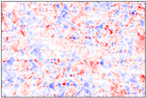
The instantaneous fields of the normalised fluctuating pressure  ${p}^{\prime }/\bar {p}$ at $y^{*}=2$ are plotted in figure 3. The TAPNS of the fluctuating pressure marked by the black dashed box in figures 3(c) and 3(d) are only abundant in the strongly cooled wall cases (i.e. ‘M8T04-Re860’ and ‘M8T015-Re2282’) and disappear in the nearly adiabatic wall cases (i.e. ‘M8T08’ cases). Furthermore, the intensities of the TAPNS of the fluctuating pressure are strongly enhanced as the wall temperature decreases.

Figure 3. Instantaneous fields of the normalised fluctuating pressure  ${p}^{\prime }/\bar {p}$ at $y^{*}=2$ in (a) ‘M8T08H-Re1315’, (b) ‘M8T08H-Re992’, (c) ‘M8T04-Re860’ and (d) ‘M8T015-Re2282’.
The dimensionless entropy per unit mass  $s$ can be defined as $s=C_{v}\log ( T/\rho ^{\gamma -1} )$ (Gerolymos & Vallet Reference Gerolymos and Vallet2014; Wang et al. Reference Wang, Wan, Chen, Xie, Wang and Chen2019). Here we define $\bar {s}$ is the spanwise and time average of the dimensionless entropy per unit mass $s$ at each wall-normal location, and the fluctuating entropy is ${s}'=s-\bar {s}$. It is pointed out by Gerolymos & Vallet (Reference Gerolymos and Vallet2014) that the fluctuating entropy $s^{\prime }$ can be approximated as a function of the relative fluctuations ${\rho }'/\bar {\rho }$ and ${T}'/\bar {T}$. Only the fluctuating entropy has a physical meaning (Gerolymos & Vallet Reference Gerolymos and Vallet2014). The instantaneous fields of the normalised fluctuating entropy $s^{\prime }\gamma M^{2}$ at $y^{*}=2$ are plotted in figure 4. It is found that the streaky structures are popular in the strongly cooled wall cases (i.e. ‘M8T04-Re860’ and ‘M8T015-Re2282’) and non-existent in the nearly adiabatic wall cases (i.e. ‘M8T08’ cases). As the wall temperature decreases, the intensities of the streaky structures are also enhanced. Specifically, the streaky structures found in the instantaneous fields of $s^{\prime }\gamma M^{2}$ in ‘M8T015-Re2282’ (figure 4d) are similar to the streaky structures of $u^{\prime }/u_{\tau }^{*}$ in ‘M8T015-Re2282’ (figure 2d). However, the TAPNSs found in the fluctuating streamwise velocity (figure 2d) are not found in the fluctuating entropy $s^{\prime }\gamma M^{2}$.

Figure 4. Instantaneous fields of the normalised fluctuating entropy  $s^{\prime }\gamma M^{2}$ at $y^{*}=2$ in (a) ‘M8T08H-Re1315’, (b) ‘M8T08H-Re992’, (c) ‘M8T04-Re860’ and (d) ‘M8T015-Re2282’.
In our recent study (Xu, Wang & Chen Reference Xu, Wang and Chen2023a), it was observed that the TAPNSs are found in the fluctuating pressure and the acoustic modes of density and temperature. The TAPNSs are short and fat structures where the characteristic streamwise length scale is smaller than the characteristic spanwise spacing scale, as shown in the black dashed boxes in figures 3(c) and 3(d). Furthermore, the TAPNSs are located at the wall and in the vicinity of the wall. As the wall-normal location  $y^{*}$ increases, the intensities of TAPNSs significantly decrease. However, the streaky structures in figures 4(c) and 4(d) are observed in the fluctuating entropy and the entropic modes of density and temperature. Therefore, the streaky structures are named as ‘streaky entropic structures’ (SESs) by Xu et al. (Reference Xu, Wang and Chen2023a). The SESs are long and thin structures where the characteristic streamwise length scale is significantly larger than the characteristic spanwise spacing scale, as shown in figure 4(d). The SESs are relatively weak at the wall and have the strongest intensities slightly away from the wall. Moreover, the SESs are mainly caused by the advection effect of the strong positive wall-normal gradient of the mean temperature associated with ejection and sweep events.
The instantaneous fields of the normalised fluctuating density  ${\rho }^{\prime }/\bar {\rho }$ and the normalised fluctuating temperature ${T}^{\prime }/\bar {T}$ at $y^{*}=2$ are shown in figures 5 and 6, respectively. The SESs and TAPNSs are all found in the instantaneous fields of the fluctuating density and temperature, and some representatives of TAPNSs are revealed by the black dashed boxes, which are located in the same regions as the black dashed boxes in the instantaneous fields of the fluctuating pressure (figure 3c,d) and the fluctuating streamwise velocity (figure 2c,d).

Figure 5. Instantaneous fields of the normalised fluctuating density  ${\rho }^{\prime }/\bar {\rho }$ at $y^{*}=2$ in (a) ‘M8T08H-Re1315’, (b) ‘M8T08H-Re992’, (c) ‘M8T04-Re860’ and (d) ‘M8T015-Re2282’.

Figure 6. Instantaneous fields of the normalised fluctuating temperature  ${T}^{\prime }/\bar {T}$ at $y^{*}=2$ in (a) ‘M8T08H-Re1315’, (b) ‘M8T08H-Re992’, (c) ‘M8T04-Re860’ and (d) ‘M8T015-Re2282’.
The instantaneous fields of the normalised fluctuating streamwise velocity  $u^{\prime }/u_{\tau }^{*}$ at $y/\delta =0.8$ are shown in figure 7. Near the edge of the boundary layer ( $y/\delta =0.8$), the instantaneous fields of $u^{\prime }/u_{\tau }^{*}$ become significantly intermittent, which are similar to the supersonic turbulent boundary layers (Pirozzoli & Bernardini Reference Pirozzoli and Bernardini2011). Some regions of the instantaneous fields of $u^{\prime }/u_{\tau }^{*}$ are quite quiescent, where the free stream irrotational flows insert into the inner rotational motions. The structures of $u^{\prime }/u_{\tau }^{*}$ at $y/\delta =0.8$ exhibit the high- and low-speed velocity streaks scaled with $\delta$, which correspond to the large-scale motions (LSMs) and very-large-scale motions (VLSMs) widely found in incompressible and compressible wall-bounded flows (Ganapathisubramani, Clemens & Dolling Reference Ganapathisubramani, Clemens and Dolling2006; Hutchins & Marusic Reference Hutchins and Marusic2007a,Reference Hutchins and Marusicb; Pirozzoli & Bernardini Reference Pirozzoli and Bernardini2011; Bross et al. Reference Bross, Scharnowski and Kähler2021).

Figure 7. Instantaneous fields of the normalised fluctuating streamwise velocity  $u^{\prime }/u_{\tau }^{*}$ at $y/\delta =0.8$ in (a) ‘M8T08H-Re1315’, (b) ‘M8T08H-Re992’, (c) ‘M8T04-Re860’ and (d) ‘M8T015-Re2282’.
The instantaneous fields of the normalised fluctuating pressure  ${p}^{\prime }/\bar {p}$ at $y/\delta =0.8$ are plotted in figure 8. Near the edge of the boundary layer, the intensities of the normalised fluctuating pressure are relatively weak. As the wall temperature decreases, the high-pressure regions are significantly enhanced.

Figure 8. Instantaneous fields of the normalised fluctuating pressure  ${p}^{\prime }/\bar {p}$ at $y/\delta =0.8$ in (a) ‘M8T08H-Re1315’, (b) ‘M8T08H-Re992’, (c) ‘M8T04-Re860’ and (d) ‘M8T015-Re2282’.
The instantaneous fields of the normalised fluctuating entropy  $s^{\prime }\gamma M^{2}$, the normalised fluctuating density ${\rho }^{\prime }/\bar {\rho }$ and the normalised fluctuating temperature ${T}^{\prime }/\bar {T}$ at $y/\delta =0.8$ are shown in figures 9, 10 and 11, respectively. It is found that the instantaneous fields of the normalised fluctuating entropy $s^{\prime }\gamma M^{2}$ (figure 9) are negatively correlated with those of the normalised fluctuating density ${\rho }^{\prime }/\bar {\rho }$ (figure 10), while positively correlated with those of the normalised fluctuating temperature ${T}^{\prime }/\bar {T}$ (figure 11) at $y/\delta =0.8$. Moreover, it is found that as the Reynolds number decreases and as the wall temperature decreases, more low-temperature structures from the free stream flows erupt into the inner high-temperature regions among the turbulent boundary layer.

Figure 9. Instantaneous fields of the normalised fluctuating entropy  $s^{\prime }\gamma M^{2}$ at $y/\delta =0.8$ in (a) ‘M8T08H-Re1315’, (b) ‘M8T08H-Re992’, (c) ‘M8T04-Re860’ and (d) ‘M8T015-Re2282’.

Figure 10. Instantaneous fields of the normalised fluctuating density  ${\rho }^{\prime }/\bar {\rho }$ at $y/\delta =0.8$ in (a) ‘M8T08H-Re1315’, (b) ‘M8T08H-Re992’, (c) ‘M8T04-Re860’ and (d) ‘M8T015-Re2282’.

Figure 11. Instantaneous fields of the normalised fluctuating temperature  ${T}^{\prime }/\bar {T}$ at $y/\delta =0.8$ in (a) ‘M8T08H-Re1315’, (b) ‘M8T08H-Re992’, (c) ‘M8T04-Re860’ and (d) ‘M8T015-Re2282’.
4. Turbulent intensities of the streamwise velocity and thermodynamic variables
The turbulent Mach number can be defined as  $M_{t}=\sqrt {\overline {{u}''_{i}{u}''_{i}}}/\bar {c}$, where $c$ represents the local sound speed. The turbulent Mach number $M_{t}$ and the normalised turbulent intensity of the streamwise velocity $u _{rms}^{\prime }/u_{\tau }^{*}$ along the wall-normal direction are shown in figure 12. It is found in figure 12(a) that the turbulent Mach number slightly increases as the Reynolds number decreases, which is consistent with previous observations (Bernardini & Pirozzoli Reference Bernardini and Pirozzoli2011b). Moreover, $M_{t}$ is significantly enhanced as the wall temperature decreases, as reported in many previous studies (Zhang et al. Reference Zhang, Duan and Choudhari2018; Xu et al. Reference Xu, Wang, Wan, Yu, Li and Chen2021a,Reference Xu, Wang, Wan, Yu, Li and Chenb, Reference Xu, Wang, Yu, Li and Chen2022b,Reference Xu, Wang, Yu, Li and Chenc,Reference Xu, Wang and Chena; Huang et al. Reference Huang, Duan and Choudhari2022; Zhang et al. Reference Zhang, Wan, Liu, Sun and Lu2022). It is shown in figure 12(b) that the Reynolds number has a negligible effect on the normalised intensity of the fluctuating streamwise velocity, while the peak value of $u _{rms}^{\prime }/u_{\tau }^{*}$ slightly increases as the wall temperature decreases, similar to previous observations (Duan et al. Reference Duan, Beekman and Martin2010; Lagha et al. Reference Lagha, Kim, Eldredge and Zhong2011; Zhang et al. Reference Zhang, Duan and Choudhari2018).

Figure 12. (a) Turbulent Mach number  $M_{t}$ along the wall-normal direction. (b) Normalised turbulent intensity of the streamwise velocity $u _{rms}^{\prime }/u_{\tau }^{*}$ along the wall-normal direction.
The normalised relative turbulent intensities  $\rho _{rms}^{\prime }/\bar {\rho }$, $T _{rms}^{\prime }/\bar {T}$ and $s _{rms}^{\prime }\gamma M^{2}$ along the wall-normal direction are shown in figure 13. It is found that the normalised turbulent intensities $\rho _{rms}^{\prime }/\bar {\rho }$, $T _{rms}^{\prime }/\bar {T}$ and $s _{rms}^{\prime }\gamma M^{2}$ have similar behaviour. Specifically, the turbulent intensities $\rho _{rms}^{\prime }/\bar {\rho }$, $T _{rms}^{\prime }/\bar {T}$ and $s _{rms}^{\prime }\gamma M^{2}$ achieve their peaks near the edge of the boundary layer, and the peak values decrease as the Reynolds number increases and as the wall temperature decreases. These observations are consistent with the instantaneous fields of $s^{\prime }\gamma M^{2}$, ${\rho }^{\prime }/\bar {\rho }$ and ${T}^{\prime }/\bar {T}$ at $y/\delta =0.8$ shown in figures 9, 10 and 11, respectively. It is found in figures 9, 10 and 11 that the magnitudes of $s^{\prime }\gamma M^{2}$, ${\rho }^{\prime }/\bar {\rho }$ and ${T}^{\prime }/\bar {T}$ become much smaller as the Reynolds number increases and as the wall temperature decreases, which further lead to the smaller values of $\rho _{rms}^{\prime }/\bar {\rho }$, $T _{rms}^{\prime }/\bar {T}$ and $s _{rms}^{\prime }\gamma M^{2}$ with larger Reynolds number and colder wall temperature near the edge of the boundary layer. Furthermore, the secondary peak values of $\rho _{rms}^{\prime }/\bar {\rho }$, $T _{rms}^{\prime }/\bar {T}$ and $s _{rms}^{\prime }\gamma M^{2}$ appear at $y^{*}=40\unicode{x2013}50$, and these secondary peak values also decrease as the Reynolds number increases and as the wall temperature decreases. However, in the near-wall region, the intensities of $\rho _{rms}^{\prime }/\bar {\rho }$, $T _{rms}^{\prime }/\bar {T}$ and $s _{rms}^{\prime }\gamma M^{2}$ significantly increase as the wall temperature decreases, and are slightly enhanced as the Reynolds number decreases. Accordingly, it is concluded that the intensities of $\rho _{rms}^{\prime }/\bar {\rho }$, $T _{rms}^{\prime }/\bar {T}$ and $s _{rms}^{\prime }\gamma M^{2}$ are enhanced as the Reynolds number decreases, while the degree of the enhancement is significantly smaller near the wall (nearly $y^{*}<10$) than that far from the wall. In contrast, as the wall temperature decreases, the intensities of $\rho _{rms}^{\prime }/\bar {\rho }$, $T _{rms}^{\prime }/\bar {T}$ and $s _{rms}^{\prime }\gamma M^{2}$ become significantly larger in the near-wall region (almost $y^{*}<10$), while they become smaller in the far-wall region. The enhancement of $s _{rms}^{\prime }\gamma M^{2}$ with colder wall temperature near the wall can be ascribed to the appearance of the SESs as shown in figure 4, and the increase of $\rho _{rms}^{\prime }/\bar {\rho }$ and $T _{rms}^{\prime }/\bar {T}$ in the near-wall region as the wall temperature decreases can be attributed to the existence of the TAPNSs and SESs, as depicted in figures 5 and 6.

Figure 13. (a,d) Normalised relative turbulent intensity of the density  $\rho _{rms}^{\prime }/\bar {\rho }$ along the wall-normal direction against (a) semi-local scaling ( $y^{*}$) and (d) outer scaling ( $y/\delta$). (b,e) Normalised relative turbulent intensity of the temperature $T _{rms}^{\prime }/\bar {T}$ along the wall-normal direction against (b) semi-local scaling ( $y^{*}$) and (e) outer scaling ( $y/\delta$). (c,f) Normalised turbulent intensity of the entropy $s _{rms}^{\prime }\gamma M^{2}$ along the wall-normal direction against (c) semi-local scaling ( $y^{*}$) and (f) outer scaling ( $y/\delta$).
The normalised relative turbulent intensity of the pressure  $p _{rms}^{\prime }/\bar {p}$ along the wall-normal direction is plotted in figure 14. The behaviour of $p _{rms}^{\prime }/\bar {p}$ is significantly different from those of $\rho _{rms}^{\prime }/\bar {\rho }$, $T _{rms}^{\prime }/\bar {T}$ and $s _{rms}^{\prime }\gamma M^{2}$. It is found that in the nearly adiabatic cases (i.e. M8T08 cases), the intensities of $p _{rms}^{\prime }/\bar {p}$ attain their peak at $y^{*}\approx 60$ and then drastically decrease as $y^{*}$ increases. Furthermore, the values of $p _{rms}^{\prime }/\bar {p}$ slightly increase as the Reynolds number decreases. However, in the strongly cooled wall cases (i.e. ‘M8T04-Re860’ and ‘M8T015-Re2282’), the intensities of $p _{rms}^{\prime }/\bar {p}$ also have local maximum values at $y^{*}\approx 60$, while the peak values of $p _{rms}^{\prime }/\bar {p}$ appear at the wall, mainly due to the appearance of TAPNSs, as shown in figure 3. Moreover, the values of $p _{rms}^{\prime }/\bar {p}$ are significantly enhanced as the wall temperature decreases, especially in the near-wall region.

Figure 14. Normalised relative turbulent intensity of the pressure  $p _{rms}^{\prime }/\bar {p}$ along the wall-normal direction against (a) semi-local scaling ( $y^{*}$) and (b) outer scaling ( $y/\delta$).
According to the Kovasznay decomposition, the fluctuating density and temperature can be decomposed into the acoustic and entropic modes. The correlation coefficients  $R ( \rho _{I} ^{\prime },T _{I}^{\prime } )$, $R ( \rho _{I} ^{\prime },p^{\prime } )$, $R ( \rho _{E} ^{\prime },T _{E}^{\prime } )$ and $R ( \rho _{E} ^{\prime },s^{\prime } )$ along the wall-normal direction are shown in figure 15. It can be seen that $R ( \rho _{I} ^{\prime },T _{I}^{\prime } )$ and $R ( \rho _{I} ^{\prime },p^{\prime } )$ are equal to 1, suggesting that $\rho _{I} ^{\prime }$ and $T _{I}^{\prime }$ are positively linearly correlated with $p^{\prime }$. Furthermore, $R ( \rho _{E} ^{\prime },T _{E}^{\prime } )$ and $R ( \rho _{E} ^{\prime },s^{\prime } )$ are almost equal to $-1$, indicating that $\rho _{E} ^{\prime }$ is almost negatively linearly correlated with $T _{E}^{\prime }$ and $s^{\prime }$.

Figure 15. Correlation coefficients (a)  $R ( \rho _{I} ^{\prime },T _{I}^{\prime } )$, (b) $R ( \rho _{I} ^{\prime },p^{\prime } )$, (c) $R ( \rho _{E} ^{\prime },T _{E}^{\prime } )$ and (d) $R ( \rho _{E} ^{\prime },s^{\prime } )$ along the wall-normal direction.
The relative normalised turbulent intensities  $\rho _{I,rms}^{\prime }/\bar {\rho }$, $\rho _{E,rms}^{\prime }/\bar {\rho }$, $T _{I,rms}^{\prime }/\bar {T}$ and $T _{E,rms}^{\prime }/\bar {T}$ along the wall-normal direction are shown in figure 16. It is found that the behaviour of the acoustic modes $\rho _{I,rms}^{\prime }/\bar {\rho }$ and $T _{I,rms}^{\prime }/\bar {T}$ are similar to that of the fluctuating pressure $p _{rms}^{\prime }/\bar {p}$, and the behaviour of the entropic modes $\rho _{E,rms}^{\prime }/\bar {\rho }$ and $T _{E,rms}^{\prime }/\bar {T}$ are similar to that of the fluctuating entropy $s _{rms}^{\prime }\gamma M^{2}$. These observations are consistent with linear correlations between the acoustic modes and the fluctuating pressure as well as between the entropic modes and the fluctuating entropy (figure 15).

Figure 16. Relative normalised turbulent intensity of (a) the acoustic mode of density  $\rho _{I,rms}^{\prime }/\bar {\rho }$, (b) the entropic mode of density $\rho _{E,rms}^{\prime }/\bar {\rho }$, (c) the acoustic mode of temperature $T _{I,rms}^{\prime }/\bar {T}$ and (d) the entropic mode of temperature $T _{E,rms}^{\prime }/\bar {T}$ along the wall-normal direction.
The relative contributions  $\rho _{E,rms}^{\prime }/ (\rho _{E,rms}^{\prime }+ \rho _{I,rms}^{\prime } )$ and $T _{E,rms}^{\prime }/ (T _{E,rms}^{\prime }+T _{I,rms}^{\prime } )$ along the wall-normal direction are shown in figure 17. It is noted that if the relative contributions $\rho _{E,rms}^{\prime }/ (\rho _{E,rms}^{\prime }+ \rho _{I,rms}^{\prime } )$ and $T _{E,rms}^{\prime }/ (T _{E,rms}^{\prime }+T _{I,rms}^{\prime } )$ are larger than 0.5, the entropic modes of the density and temperature are predominant over their acoustic modes; and vice versa. It is found that at $y^{*}>20$, the relative contributions $\rho _{E,rms}^{\prime }/ (\rho _{E,rms}^{\prime }+ \rho _{I,rms}^{\prime } )$ and $T _{E,rms}^{\prime }/ (T _{E,rms}^{\prime }+T _{I,rms}^{\prime } )$ are larger than 0.5, indicating the dominance of the entropic modes of density and temperature among most regions of the boundary layer. As the wall-normal location increases, the values of the relative contributions $\rho _{E,rms}^{\prime }/ (\rho _{E,rms}^{\prime }+ \rho _{I,rms}^{\prime } )$ and $T _{E,rms}^{\prime }/ (T _{E,rms}^{\prime }+T _{I,rms}^{\prime } )$ slightly increase, suggesting that the dominance of the entropic modes of density and temperature is slightly enhanced away from the wall. Furthermore, in the far-wall region, the values of the relative contributions $\rho _{E,rms}^{\prime }/ (\rho _{E,rms}^{\prime }+ \rho _{I,rms}^{\prime } )$ and $T _{E,rms}^{\prime }/ (T _{E,rms}^{\prime }+T _{I,rms}^{\prime } )$ slightly increase as the Reynolds number decreases, while they significantly decrease as the wall temperature decreases. However, in the near-wall region $y^{*}<20$, the acoustic modes of density and temperature have significant contributions. It is found that the relative contributions of the acoustic modes of density and temperature decrease as the wall temperature decreases. This observation can be attributed to the appearance of the SESs near the wall in the strongly cooled wall cases. It is shown in figures 5 and 6 that although both the SESs and TAPNSs appear in the near-wall region in the ‘M8T04-Re860’ and ‘M8T015-Re2282’ cases, the intensities and the volume fractions of the SESs are much stronger than those of the TAPNSs, which further lead to the larger relative contributions of the entropic modes of density and temperature as the wall temperature decreases.

Figure 17. Relative contributions (a)  $\rho _{E,rms}^{\prime }/ (\rho _{E,rms}^{\prime }+ \rho _{I,rms}^{\prime } )$ and (b) $T _{E,rms}^{\prime }/ (T _{E,rms}^{\prime }+T _{I,rms}^{\prime } )$ along the wall-normal direction.
5. The p.d.f.s of the streamwise velocity and the thermodynamic variables
The p.d.f.s along the wall-normal direction are discussed in this section. It is noted that the total numbers of samples used for the computation of the p.d.f.s at each wall-normal location in ‘M8T08H-Re1315’, ‘M8T08H-Re992’, ‘M8T04-Re860’ and ‘M8T015-Re2282’ are  $4.8\times 10^{7}$, $2.88\times 10^{7}$, $5.76\times 10^{7}$ and $1.54\times 10^{8}$, respectively.
The p.d.f.s of  $u^{\prime }/u^{\prime }_{rms}$ are shown in figure 18. It is noted that the colourful contours in figures 18(a) and 18(b) represent the p.d.f. of $u^{\prime }/u^{\prime }_{rms}$ in ‘M8T08H-Re1315’, and the line contours represent the p.d.f.s of $u^{\prime }/u^{\prime }_{rms}$ in ‘M8T08H-Re1315’, ‘M8T08H-Re992’, ‘M8T04-Re860’ and ‘M8T015-Re2282’, with the line symbols consistent with the legend in figure 18(c). It is shown in figure 18(a) that the p.d.f.s of $u^{\prime }/u^{\prime }_{rms}$ are strongly positively skewed near the wall. As the wall-normal location $y^{*}$ increases, the skewness of $u^{\prime }/u^{\prime }_{rms}$ decreases to zero at $y^{*} \approx 10$ and then becomes negative. This behaviour is consistent with the skewness of $u^{\prime }$ shown by Huang et al. (Reference Huang, Duan and Choudhari2022) and Pirozzoli & Bernardini (Reference Pirozzoli and Bernardini2011). In the near-wall region, the instantaneous fields of $u^{\prime }/u_{\tau }^{*}$ (figure 2) show that the magnitudes of the positive values of $u^{\prime }/u_{\tau }^{*}$ are much larger than those of the negative values, indicating that the high momentum streaks have much stronger intensities than the low momentum streaks. This observation further gives rise to the strong positive skewness of $u^{\prime }/u^{\prime }_{rms}$ near the wall. However, in the far-wall region, the instantaneous fields of $u^{\prime }/u_{\tau }^{*}$ (figure 7) reveal that the magnitudes of the negative values of $u^{\prime }/u_{\tau }^{*}$ are much larger than those of the positive values. Furthermore, the weak high-speed events are dominant, while the low-speed events are more intense, but rarer (Pirozzoli & Bernardini Reference Pirozzoli and Bernardini2011). These observations further lead to the strong negative skewness of $u^{\prime }/u^{\prime }_{rms}$ near the edge of the boundary layer. Near the edge of the boundary layer, the negative values of $u^{\prime }/u_{\tau }^{*}$ represent the rotational motions inside the boundary layer, while the strong positive values indicate the free stream irrotational flows outside the boundary layer (Huang et al. Reference Huang, Duan and Choudhari2022). Thus, the strong negative skewness of $u^{\prime }/u_{\tau }^{*}$ indicates that the rotational motions inside the boundary layer have much stronger intensities than the free stream irrotational flows outside the boundary layer. Furthermore, it is found that the four different line contours in figures 18(a) and 18(b) are similar to each other at least for the p.d.f. contour levels between $10^{-2}$ and $10^{-1}$, which indicates that the Reynolds number and wall temperature have relatively small influences on the distribution of $u^{\prime }/u^{\prime }_{rms}$. This observation can be further verified in the p.d.f.s of $u^{\prime }/u^{\prime }_{rms}$ at $y^{*}=2$ and $y/\delta =0.8$ shown in figures 18(c) and 18(d). It is seen in figures 18(c) and 18(d) that the p.d.f.s of $u^{\prime }/u^{\prime }_{rms}$ in the above four cases almost collapse when the value of the p.d.f. is larger than $10^{-3}$. It is also found in figure 18(d) that as the Reynolds number and wall temperature decrease, the negative tails of the p.d.f.s of $u^{\prime }/u^{\prime }_{rms}$ become shorter at $y/\delta =0.8$. This can be attributed to the reason that as the Reynolds number and wall temperature decrease, more free stream irrotational flows insert into the inner rotational motions, and the magnitudes of the negative values of $u^{\prime }/u_{\tau }^{*}$ become smaller (figure 7).

Figure 18. (a,b) The p.d.f.s of  $u^{\prime }/u^{\prime }_{rms}$ along the wall-normal direction with (a) semi-local scaling ( $y^{*}$) and (b) outer scaling ( $y/\delta$). The vertical dashed lines represent $y^{*}=2$ in panel (a) and $y/\delta =0.8$ in panel (b). (c,d) The p.d.f.s of $u^{\prime }/u^{\prime }_{rms}$ at (c) $y^{*}=2$ and (d) $y/\delta =0.8$. The colourful contours in panels (a,b) represent the p.d.f. of $u^{\prime }/u^{\prime }_{rms}$ in ‘M8T08H-Re1315’. The line contours in panels (a,b) represent the p.d.f.s of $u^{\prime }/u^{\prime }_{rms}$ in four cases, and the line symbols are consistent with the legend in panel (c). The line contour levels in panels (a,b) are ( $10^{-4}$, $10^{-3}$, $10^{-2}$, $10^{-1}$).
The p.d.f.s of  $p^{\prime }/p ^{\prime }_{rms}$ are shown in figure 19. It is found that the p.d.f.s of $p^{\prime }/p ^{\prime }_{rms}$ are much more symmetric than those of $s^{\prime }/s ^{\prime }_{rms}$, $\rho ^{\prime }/\rho ^{\prime }_{rms}$ and $T^{\prime }/T ^{\prime }_{rms}$ shown in figures 20, 21 and 22 later, indicating that the high-pressure events have comparable intensities with the low-pressure events along the wall-normal direction. In the near-wall region, the p.d.f.s of $p^{\prime }/p ^{\prime }_{rms}$ are almost symmetric in the nearly adiabatic cases (‘M8T08’ cases). This is consistent with the instantaneous fields of ${p}^{\prime }/\bar {p}$ at $y^{*}=2$ (figure 3a,b), where the negative values of ${p}^{\prime }/\bar {p}$ have similar magnitudes with the positive values. It is noted that this behaviour is consistent with the symmetric p.d.f.s of the wall pressure in incompressible channel flows (Hu, Morfey & Sandham Reference Hu, Morfey and Sandham2006) and nearly adiabatic compressible turbulent boundary layer (Zhang et al. Reference Zhang, Wan, Liu, Sun and Lu2022). As the wall temperature decreases, the TAPNSs appear near the wall, and it is found in figures 3(c) and 3(d) that the positive values of ${p}^{\prime }/\bar {p}$ have much stronger magnitudes than the negative values among the TAPNSs. Therefore, the skewness of $p^{\prime }/p ^{\prime }_{rms}$ becomes much more positive as the wall temperature decreases, which is consistent with the positive skewed p.d.f.s of the wall pressure in a compressible turbulent boundary layer with cooled wall (Zhang et al. Reference Zhang, Wan, Liu, Sun and Lu2022). In the far-wall region, the intensities of $p _{rms}^{\prime }/\bar {p}$ significantly decrease with the increase of $y^{*}$ and become pretty weak near the edge of the boundary layer. It is found in figure 8 that the magnitudes of the positive values of ${p}^{\prime }/\bar {p}$ are similar to those of the negative values at $y/\delta =0.8$. Accordingly, the p.d.f.s of $p^{\prime }/p ^{\prime }_{rms}$ are nearly symmetric at $y/\delta =0.8$. Moreover, the Reynolds number and wall temperature have a pretty small effect on the distribution of $p^{\prime }/p ^{\prime }_{rms}$ in the far-wall region.

Figure 19. (a,b) The p.d.f.s of  $p^{\prime }/p ^{\prime }_{rms}$ along the wall-normal direction with (a) semi-local scaling ( $y^{*}$) and (b) outer scaling ( $y/\delta$). The vertical dashed lines represent $y^{*}=2$ in panel (a) and $y/\delta =0.8$ in panel (b). (c,d) The p.d.f.s of $p^{\prime }/p ^{\prime }_{rms}$ at (c) $y^{*}=2$ and (d) $y/\delta =0.8$. The colourful contours in panels (a,b) represent the p.d.f. of $p^{\prime }/p ^{\prime }_{rms}$ in ‘M8T08H-Re1315’. The line contours in panels (a,b) represent the p.d.f.s of $p^{\prime }/p ^{\prime }_{rms}$ in four cases, and the line symbols are consistent with the legend in panel (c). The line contour levels in panels (a,b) are ( $10^{-4}, 10^{-3}, 10^{-2}, 10^{-1}$).

Figure 20. (a,b) The p.d.f.s of  $s^{\prime }/s ^{\prime }_{rms}$ along the wall-normal direction with (a) semi-local scaling ( $y^{*}$) and (b) outer scaling ( $y/\delta$). The vertical dashed lines represent $y^{*}=2$ in panel (a) and $y/\delta =0.8$ in panel (b). (c,d) The p.d.f.s of $s^{\prime }/s ^{\prime }_{rms}$ at (c) $y^{*}=2$ and (d) $y/\delta =0.8$. The colourful contours in panels (a,b) represent the p.d.f. of $s^{\prime }/s ^{\prime }_{rms}$ in ‘M8T08H-Re1315’. The line contours in panels (a,b) represent the p.d.f.s of $s^{\prime }/s ^{\prime }_{rms}$ in four cases, and the line symbols are consistent with the legend in panel (c). The line contour levels in panels (a,b) are ( $10^{-4}$, $10^{-3}$, $10^{-2}$, $10^{-1}$). (e) Mean density profile and (f) mean temperature profile along the wall-normal direction.

Figure 21. (a,b) The p.d.f.s of  $\rho ^{\prime }/\rho ^{\prime }_{rms}$ along the wall-normal direction with (a) semi-local scaling ( $y^{*}$) and (b) outer scaling ( $y/\delta$). The vertical dashed lines represent $y^{*}=2$ in panel (a) and $y/\delta =0.8$ in panel (b). (c,d) The p.d.f.s of $\rho ^{\prime }/\rho ^{\prime }_{rms}$ at (c) $y^{*}=2$ and (d) $y/\delta =0.8$. The colourful contours in panels (a,b) represent the p.d.f.s of $\rho ^{\prime }/\rho ^{\prime }_{rms}$ in ‘M8T08H-Re1315’. The line contours in panels (a,b) represent the p.d.f. of $\rho ^{\prime }/\rho ^{\prime }_{rms}$ in four cases and the line symbols are consistent with the legend in panel (c). The line contour levels in panels (a,b) are ( $10^{-4}, 10^{-3}, 10^{-2}, 10^{-1}$).

Figure 22. (a,b) The p.d.f.s of  $T^{\prime }/T ^{\prime }_{rms}$ along the wall-normal direction with (a) semi-local scaling ( $y^{*}$) and (b) outer scaling ( $y/\delta$). The vertical dashed lines represent $y^{*}=2$ in panel (a) and $y/\delta =0.8$ in panel (b). (c,d) The p.d.f.s of $T^{\prime }/T ^{\prime }_{rms}$ at (c) $y^{*}=2$ and (d) $y/\delta =0.8$. The colourful contours in panels (a,b) represent the p.d.f. of $T^{\prime }/T ^{\prime }_{rms}$ in ‘M8T08H-Re1315’. The line contours in panels (a,b) represent the p.d.f.s of $T^{\prime }/T ^{\prime }_{rms}$ in four cases and the line symbols are consistent with the legend in panel (c). The line contour levels in panels (a,b) are ( $10^{-4}, 10^{-3}, 10^{-2}, 10^{-1}$).
The p.d.f.s of  $s^{\prime }/s ^{\prime }_{rms}$ are shown in figure 20. It is found that in the nearly adiabatic cases (‘M8T08’ cases), the p.d.f.s of $s^{\prime }/s ^{\prime }_{rms}$ are negatively skewed near the wall and the degree of the negative skewness becomes larger as $y^{*}$ increases. The negative skewness of $s^{\prime }/s ^{\prime }_{rms}$ near the wall is consistent with the instantaneous fields of $s^{\prime }\gamma M^{2}$ at $y^{*}=2$ in figures 4(a) and 4(b), where the negative values of $s^{\prime }\gamma M^{2}$ have larger magnitudes than the positive values. In the strongly cooled wall cases, the SESs appear near the wall. It is shown in figures 4(c) and 4(d) that the positive values of $s^{\prime }\gamma M^{2}$ have stronger magnitudes than the negative values among the SESs, which lead to the much larger values of the skewness of $s^{\prime }/s ^{\prime }_{rms}$ in ‘M8T04-Re860’ and ‘M8T015-Re2282’ than those in ‘M8T08’ cases (figure 20a). The above observations can be qualitatively explained as follows: it is found in figure 20(f) that the values of the mean temperatures in nearly adiabatic cases (‘M8T08’ cases) are significantly larger than those in strongly cooled wall cases. Therefore, due to the physical limits that $T>0$ and $\rho >0$, the magnitudes of the low-entropy events in nearly adiabatic cases should be significantly larger than those in strongly cooled wall cases, which is consistent with the much longer negative tails in ‘M8T08’ cases in figure 20(c). Accordingly, the cold wall significantly restricts the intensities of the low-entropy events and then generates the SESs, which further leads to the much larger values of the skewness of $s^{\prime }/s ^{\prime }_{rms}$ near the wall in strongly cooled wall cases. It is also found that the wall-normal locations where the skewness of the p.d.f.s of $s^{\prime }/s ^{\prime }_{rms}$ have the smallest values are similar to the wall-normal locations where the mean density profiles attain the minimum values (figure 20e) and the mean temperature profiles obtain the maximum values (figure 20f). After achieving the largest negative values of the skewness, the values of the skewness increase as $y^{*}$ increases. Near the edge of the boundary layer, it is noted that the positive values of $s^{\prime }\gamma M^{2}$ represent the flows inside the boundary layer, while the strong negative values indicate the free stream flows outside the boundary layer. The instantaneous fields of $s^{\prime }\gamma M^{2}$ at $y/\delta =0.8$ (figure 9) show that the magnitudes of the positive values of $s^{\prime }\gamma M^{2}$ are much stronger than those of the negative values, which further give rise to the strong positive skewness of the p.d.f.s of $s^{\prime }/s ^{\prime }_{rms}$. It means that near the edge of the boundary layer, the high-entropy motions inside the boundary layer have significantly larger intensities than the low-entropy motions outside the boundary layer, which is fully consistent with the observation found in $u^{\prime }/u_{\tau }^{*}$ previously.
The p.d.f.s of  $\rho ^{\prime }/\rho ^{\prime }_{rms}$ are shown in figure 21. It is noted that the fluctuating density is dominant by its entropic mode among most regions of the boundary layer except for the near-wall region (figure 17), and the entropic mode of density is almost negatively linearly correlated with the fluctuating entropy (figure 15). Therefore, the p.d.f.s of $\rho ^{\prime }/\rho ^{\prime }_{rms}$ are negatively correlated with those of $s^{\prime }/s ^{\prime }_{rms}$ shown in figure 20. To be specific, the p.d.f.s of $\rho ^{\prime }/\rho ^{\prime }_{rms}$ are slightly negatively skewed near the edge of the boundary layer. This is consistent with the instantaneous fields of ${\rho }^{\prime }/\bar {\rho }$ at $y/\delta =0.8$ in figure 10, where the negative values of ${\rho }^{\prime }/\bar {\rho }$ have slightly larger magnitudes than the positive values. Furthermore, the skewness of $\rho ^{\prime }/\rho ^{\prime }_{rms}$ is positive near the wall, then increases as $y^{*}$ increases and finally reaches the maximum positive value at the wall-normal location where the mean density profile achieves the minimum value. Although in the near-wall region, the acoustic mode of density has a larger contribution than the entropic mode of density, the p.d.f.s of the acoustic mode of density and the fluctuating pressure (figure 19) are nearly symmetric. Therefore, the positive skewness of the p.d.f. of $\rho ^{\prime }/\rho ^{\prime }_{rms}$ is mainly caused by its entropic mode and is negatively linearly correlated with those of $s^{\prime }/s ^{\prime }_{rms}$. As the wall temperature decreases, the acoustic mode of density exhibits the TAPNSs at the wall and in the vicinity of the wall. Among the TAPNSs, the positive values of the acoustic mode of density have much stronger magnitudes than the negative values, which is similar to the behaviour of fluctuating pressure. This leads to the phenomenon that the positive skewness of the p.d.f. of $\rho ^{\prime }/\rho ^{\prime }_{rms}$ is enhanced as the wall temperature decreases in the vicinity of the wall. When the wall-normal location is slightly away from the wall, the entropic mode of density exhibits the SESs, while the SESs of the entropic mode of density are negatively correlated with those of the fluctuating entropy. Therefore, the negative values of the entropic mode of density have stronger magnitudes than the positive values among the SESs, which further give rise to the phenomenon that the positive skewness of the p.d.f. of $\rho ^{\prime }/\rho ^{\prime }_{rms}$ is reduced as the wall temperature decreases slightly away from the wall.
The p.d.f.s of  $T^{\prime }/T ^{\prime }_{rms}$ are plotted in figure 22. It is found that the p.d.f.s of $T^{\prime }/T ^{\prime }_{rms}$ are almost similar to those of $s^{\prime }/s ^{\prime }_{rms}$. This can be attributed to the reasons that the fluctuating temperature is dominant by its entropic mode among most regions of the boundary layer (figure 17) and the entropic mode of temperature is almost positively linearly correlated with the fluctuating entropy (figure 15). Specifically, it is found in figure 11 that the positive values of ${T}^{\prime }/\bar {T}$ have much stronger magnitudes than the negative values at $y/\delta =0.8$, which lead to the positive skewness of the p.d.f.s of $T^{\prime }/T ^{\prime }_{rms}$ near the edge of the boundary layer. In the near-wall region, the skewness of the p.d.f. of $T^{\prime }/T ^{\prime }_{rms}$ is weakly negative near the wall, then decreases as $y^{*}$ increases and finally reaches the minimum negative value at the wall-normal location where the mean temperature profile achieves the maximum value. This behaviour is similar to the variation of the p.d.f. of $s^{\prime }/s ^{\prime }_{rms}$. It is noted that the magnitudes of the skewness of $T^{\prime }/T ^{\prime }_{rms}$ are much larger than those of $\rho ^{\prime }/\rho ^{\prime }_{rms}$. This can be attributed to the reason that the relative contribution of the entropic mode to the fluctuating temperature is much larger than that of the entropic mode to the fluctuating density (figure 17); the acoustic mode is dominant in the fluctuating density near the wall and the symmetric distribution of the acoustic mode of density largely relieves the positive skewed distribution of the entropic mode of density. As the wall temperature decreases, the acoustic mode of temperature generates the TAPNSs in the vicinity of the wall. The positive values of the acoustic mode of temperature have much stronger magnitudes than the negative values among the TAPNSs, similar to the behaviour of fluctuating pressure. Therefore, the weakly negative skewness of the p.d.f. of $T^{\prime }/T ^{\prime }_{rms}$ increases to positive as the wall temperature decreases in the vicinity of the wall. As $y^{*}$ slightly increases, the entropic mode of temperature generates the SESs and the positive values of the entropic mode of temperature have stronger magnitudes than the negative values among the SESs. Accordingly, the magnitude of the negative skewness of the p.d.f. of $T^{\prime }/T ^{\prime }_{rms}$ becomes much weaker slightly away from the wall as the wall temperature decreases. The cold wall significantly suppresses the low-temperature events near the wall and then reduces the magnitude of the negative skewness of the p.d.f. of $T^{\prime }/T ^{\prime }_{rms}$ near the wall.
6. Correlation coefficients between the thermodynamic variables and the streamwise velocity
Correlation coefficients between different quantities are of particular importance not only to understand the complex interactions between different variables, but also to guide the modelling of the unclosed terms in LES and RANS (Taulbee & Vanosdol Reference Taulbee and Vanosdol1991; Wei & Pollard Reference Wei and Pollard2011; Gerolymos & Vallet Reference Gerolymos and Vallet2014, Reference Gerolymos and Vallet2018). Therefore, the correlation coefficients between the thermodynamic variables and the streamwise velocity are investigated in this section.
The correlation coefficient  $R ( p ^{\prime },s^{\prime } )$ along the wall-normal direction is shown in figure 23. The fluctuating pressure is strongly negatively correlated with the fluctuating entropy in the vicinity of the wall in the nearly adiabatic cases (i.e. ‘M8T08’ cases) and the absolute values of $R ( p ^{\prime },s^{\prime } )$ significantly decrease as $y^{*}$ increases, which is similar to the behaviour in compressible channel flows (Gerolymos & Vallet Reference Gerolymos and Vallet2014). The magnitude of $R ( p ^{\prime },s^{\prime } )$ slightly decreases as the Reynolds number decreases in the near-wall region. As the wall temperature decreases, the magnitude of $R ( p ^{\prime },s^{\prime } )$ significantly decreases in the vicinity of the wall. This can be attributed to the fact that the appearance of the TANPSs and SESs leads to the significant difference between the structures of $p ^{\prime }$ and $s^{\prime }$. As $y^{*}$ further increases, the values of $R ( p ^{\prime },s^{\prime } )$ change from negative to positive in ‘M8T04-Re860’ and ‘M8T015-Re2282’. The positive values of $R ( p ^{\prime },s^{\prime } )$ are probably attributed to the presence of the SESs. Furthermore, it is shown in figure 23(b) that the fluctuating pressure is weakly negatively correlated with the fluctuating entropy among most regions of the boundary layer, which is consistent with the behaviour in compressible channel flows (Gerolymos & Vallet Reference Gerolymos and Vallet2014). However, near the edge of the boundary layer, the absolute values of $R ( p ^{\prime },s^{\prime } )$ slightly increase mainly due to the intermittency caused by the downward incursions of the external free stream irrotational flow into the boundary layer.

Figure 23. Correlation coefficient  $R ( p ^{\prime },s^{\prime } )$ along the wall-normal direction plotted against (a) semi-local scaling ( $y^{*}$) and (b) outer scaling ( $y/\delta$).
The correlation coefficient  $R ( \rho ^{\prime },T^{\prime } )$ along the wall-normal direction is shown in figure 24. The Reynolds number has a relatively small effect on the values of $R ( \rho ^{\prime },T^{\prime } )$. In the near-wall region, $\rho ^{\prime }$ and $T^{\prime }$ are positively correlated with $R ( \rho ^{\prime },T^{\prime } )>0.5$ in the nearly adiabatic cases (i.e. ‘M8T08’ cases). As the wall temperature decreases, the values of $R ( \rho ^{\prime },T^{\prime } )$ drastically decrease near the wall. As $y^{*}$ increases, the values of $R ( \rho ^{\prime },T^{\prime } )$ significantly decrease to almost $-1$. It is shown in figure 24(b) that $R ( \rho ^{\prime },T^{\prime } ) \approx -1$ among most regions of the boundary layer, which indicates that $\rho ^{\prime }$ is almost negatively linearly correlated with $T^{\prime }$ in these regions. This observation is consistent with the negative correlation between the instantaneous fields of ${\rho }^{\prime }/\bar {\rho }$ and ${T}^{\prime }/\bar {T}$ at $y/\delta =0.8$ (figures 10 and 11).

Figure 24. Correlation coefficient  $R ( \rho ^{\prime },T^{\prime } )$ along the wall-normal direction plotted against (a) semi-local scaling ( $y^{*}$) and (b) outer scaling ( $y/\delta$). The vertical dashed line represents $y/\delta =0.8$ in panel (b).
To systematically investigate the relative contributions of the acoustic and entropic modes of density and temperature to the correlation coefficients, we introduce  $R_{p} ( \rho _{I} ^{\prime },T _{I}^{\prime } )=\overline {\rho _{I} ^{\prime }T _{I}^{\prime }}/ (\sqrt {\overline {{\rho }^{\prime 2}}}\sqrt {\overline {{T}^{\prime 2}}} )$ to represent the relative contributions of the interaction between the acoustic modes of density and temperature to $R ( \rho ^{\prime },T^{\prime } )$. Other symbols $R_{p} ( \rho _{E} ^{\prime },T _{E}^{\prime } )$, $R_{p} ( \rho _{I} ^{\prime },T _{E}^{\prime } )$ and $R_{p} ( \rho _{E} ^{\prime },T _{I}^{\prime } )$ have similar expressions and they satisfy
 \begin{equation} R_{p}\left ( \rho _{I} ^{\prime},T _{I}^{\prime} \right )+R_{p}\left ( \rho _{E} ^{\prime},T _{E}^{\prime} \right )+R_{p}\left ( \rho _{I} ^{\prime},T _{E}^{\prime} \right )+R_{p}\left ( \rho _{E} ^{\prime},T _{I}^{\prime} \right )=R\left ( \rho ^{\prime},T^{\prime} \right ). \end{equation}
 The correlation coefficient  $R ( \rho ^{\prime },T^{\prime } )$ and its relative contributions along the wall-normal direction are shown in figure 25. It is shown in figure 25(a) that the positive $R ( \rho ^{\prime },T^{\prime } )$ near the wall is mainly contributed by the interaction between $\rho _{I} ^{\prime }$ and $T _{I}^{\prime }$, while $R ( \rho ^{\prime },T^{\prime } )$ in the far-wall region is almost completely contributed by the interaction between $\rho _{E} ^{\prime }$ and $T _{E}^{\prime }$, where $R_{p} ( \rho _{E} ^{\prime },T _{E}^{\prime } ) \approx -1$. The Reynolds number has a relatively small effect on the values of $R ( \rho ^{\prime },T^{\prime } )$ and its relative contributions, while the wall temperature significantly affects the behaviour of $R ( \rho ^{\prime },T^{\prime } )$ and its relative contributions. As the wall temperature decreases, it is shown in figure 25(b) that the positive values of the relative contribution $R_{p} ( \rho _{I} ^{\prime },T _{I}^{\prime } )$ decrease significantly in the vicinity of the wall, mainly due to the smaller relative contribution of the acoustic modes to the density and temperature in strongly cooled wall cases (figure 17). This further decreases the positive values of $R ( \rho ^{\prime },T^{\prime } )$ in the vicinity of the wall. Furthermore, it is found in figure 25(c) that the profiles of $R_{p} ( \rho _{E} ^{\prime },T _{E}^{\prime } )$ in ‘M8T04-Re860’ and ‘M8T015-Re2282’ exhibit a local valley in the near-wall region, especially in ‘M8T015-Re2282’ marked by the green dashed box. This sharply increased negative correlation $R_{p} ( \rho _{E} ^{\prime },T _{E}^{\prime } )$ can be attributed to the appearance of the SESs. It should be noted that the deep valley caused by the strong SESs in the profile of $R_{p} ( \rho _{E} ^{\prime },T _{E}^{\prime } )$ in ‘M8T015-Re2282’ directly gives rise to the deep valley appearing in the profile of $R ( \rho ^{\prime },T^{\prime } )$ (marked by the green dashed box in figure 24a). Furthermore, due to the appearance of the SESs, the wall-normal location $y^{*}$ where $R_{p} ( \rho _{E} ^{\prime },T _{E}^{\prime } )$ and $R ( \rho ^{\prime },T^{\prime } )$ achieve nearly $-1$ become significantly larger as the wall temperature decreases.

Figure 25. (a) Correlation coefficient  $R ( \rho ^{\prime },T^{\prime } )$ and its relative contributions $R_{p} ( \rho _{I} ^{\prime },T _{I}^{\prime } )$, $R_{p} ( \rho _{E} ^{\prime },T _{E}^{\prime } )$, $R_{p} ( \rho _{I} ^{\prime },T _{E}^{\prime } )$ and $R_{p} ( \rho _{E} ^{\prime },T _{I}^{\prime } )$ along the wall-normal direction in ‘M8T08H-Re1315’. (b–e) Relative contributions (b) $R_{p} ( \rho _{I} ^{\prime },T _{I}^{\prime } )$, (c) $R_{p} ( \rho _{E} ^{\prime },T _{E}^{\prime } )$, (d) $R_{p} ( \rho _{I} ^{\prime },T _{E}^{\prime } )$ and (e) $R_{p} ( \rho _{E} ^{\prime },T _{I}^{\prime } )$ along the wall-normal direction in all six cases. If we define $C= (\sqrt {\overline {{\rho }^{\prime 2}}}\sqrt {\overline {{T}^{\prime 2}}} )$, then $R_{p} ( \rho _{I} ^{\prime },T _{I}^{\prime } )=\overline {\rho _{I} ^{\prime }T _{I}^{\prime }}/C$, $R_{p} ( \rho _{E} ^{\prime },T _{E}^{\prime } )=\overline {\rho _{E} ^{\prime }T _{E}^{\prime }}/C$, $R_{p} ( \rho _{I} ^{\prime },T _{E}^{\prime } )=\overline {\rho _{I} ^{\prime }T _{E}^{\prime }}/C$ and $R_{p} ( \rho _{E} ^{\prime },T _{I}^{\prime } )=\overline {\rho _{E} ^{\prime }T _{I}^{\prime }}/C$.
The correlation coefficient  $R ( \rho ^{\prime },p^{\prime } )$ along the wall-normal direction is shown in figure 26. The $\rho ^{\prime }$ is highly positively correlated with $p^{\prime }$ near the wall, which is consistent with the observation in compressible channel flows (Gerolymos & Vallet Reference Gerolymos and Vallet2014). This can be attributed to the reason that the correlation at the wall $R ( \rho ^{\prime },p^{\prime } )|_{w}$ is strictly equal to 1 (Gerolymos & Vallet Reference Gerolymos and Vallet2014). As the wall-normal location increases, $R ( \rho ^{\prime },p^{\prime } )$ significantly decreases and maintains a relatively weak positive correlation in most regions of the boundary layer. Near the edge of the boundary layer, the values of $R ( \rho ^{\prime },p^{\prime } )$ slightly increase, mainly due to the intermittency caused by the turbulent/non-turbulent interaction. It is also found that as the wall temperature decreases, $R ( \rho ^{\prime },p^{\prime } )$ slightly decreases at $y^{*} < 3$ and increases at $0.02 < y/\delta < 0.6$.

Figure 26. Correlation coefficient  $R ( \rho ^{\prime },p^{\prime } )$ along the wall-normal direction plotted against (a) semi-local scaling ( $y^{*}$) and (b) outer scaling ( $y/\delta$). The vertical dashed lines represent $y^{*}=3$ in panel (a) and $y/\delta =0.02, 0.6$ in panel (b).
The correlation coefficient  $R ( \rho ^{\prime },p^{\prime } )$ and its relative contributions $R_{p} ( \rho _{I}^{\prime },p^{\prime } )$ and $R_{p} ( \rho _{E}^{\prime },p^{\prime } )$ along the wall-normal direction are shown in figure 27. It is shown in figure 27(a) that the high positive correlation $R ( \rho ^{\prime },p^{\prime } )$ near the wall is mainly contributed by the interaction between the acoustic mode of density and the fluctuating pressure $R_{p} ( \rho _{I}^{\prime },p^{\prime } )$, while the entropic mode of density begins to give a dominant contribution to $R ( \rho ^{\prime },p^{\prime } )$ at $y^{*} >2000$ (equivalent to $y/\delta > 0.42$ in ‘M8T08H-Re1315’). Therefore, the slightly increased nature of $R ( \rho ^{\prime },p^{\prime } )$ near the edge of the boundary layer is contributed by the entropic mode of density. It is found in figure 27(b) that due to the appearance of the TAPNSs in strongly cooled wall cases, the relative contribution $R_{p} ( \rho _{I}^{\prime },p^{\prime } )$ increases, indicating a tendency to enhance $R ( \rho ^{\prime },p^{\prime } )$ with a cooled wall. However, the correlation $R ( \rho ^{\prime },p^{\prime } )$ actually decreases as the wall temperature decreases at $y^{*} < 3$ (figure 26a). This decrease nature of $R ( \rho ^{\prime },p^{\prime } )$ near the wall is mainly contributed by the entropic mode of density. It is shown in figure 27(c) that due to the appearance of the SESs in the strongly cooled wall cases, the deep valleys appear in the profiles of $R_{p} ( \rho _{E}^{\prime },p^{\prime } )$ in ‘M8T04-Re860’ and ‘M8T015-Re2282’. These observations further give rise to the decrease of $R ( \rho ^{\prime },p^{\prime } )$ as the wall temperature decreases near the wall, as well as the similar valley in the profile of $R ( \rho ^{\prime },p^{\prime } )$ in ‘M8T015-Re2282’ (marked by the green dashed box in figure 26a). Furthermore, as the wall temperature decreases, the increase of $R ( \rho ^{\prime },p^{\prime } )$ at $0.02 < y/\delta < 0.6$ is mainly contributed to the larger relative contribution of the acoustic mode of density $R_{p} ( \rho _{I}^{\prime },p^{\prime } )$ (figure 27b). However, the Reynolds number effect has a negligible effect on the value of $R ( \rho ^{\prime },p^{\prime } )$ at almost $y^{*} < 100$, while the value of $R ( \rho ^{\prime },p^{\prime } )$ is slightly enhanced at low Reynolds number at nearly $y^{*} > 100$, which is mainly caused by the entropic mode of density (figure 27c).

Figure 27. (a) Correlation coefficient  $R ( \rho ^{\prime },p^{\prime } )$ and its relative contributions $R_{p} ( \rho _{I}^{\prime },p^{\prime } )$ and $R_{p} ( \rho _{E}^{\prime },p^{\prime } )$ along the wall-normal direction in ‘M8T08H-Re1315’. (b,c) Relative contributions (b) $R_{p} ( \rho _{I}^{\prime },p^{\prime } )$ and (c) $R_{p} ( \rho _{E}^{\prime },p^{\prime } )$ along the wall-normal direction in all six cases.
The correlation coefficient  $R ( \rho ^{\prime },s^{\prime } )$ along the wall-normal direction is plotted in figure 28. The correlation $R ( \rho ^{\prime },s^{\prime } )$ has complicated variations in the near-wall region ( $y^{*}<20$). As $y^{*}$ increases, $R ( \rho ^{\prime },s^{\prime } )$ achieves almost $-1$ in most regions of the boundary layer. This is consistent with the strong negative correlation between $\rho ^{\prime }$ and $s^{\prime }$ shown in the instantaneous fields at $y/\delta =0.8$ (figures 10 and 9). Moreover, it is found that the Reynolds number has a weak effect on the values of $R ( \rho ^{\prime },s^{\prime } )$, while the wall temperature only has a significant influence on the values of $R ( \rho ^{\prime },s^{\prime } )$ in the near-wall region.

Figure 28. Correlation coefficient  $R ( \rho ^{\prime },s^{\prime } )$ along the wall-normal direction plotted against (a) semi-local scaling ( $y^{*}$) and (b) outer scaling ( $y/\delta$). The vertical dashed line represents $y/\delta =0.8$ in panel (b).
To determine the underlying mechanisms of the complicated behaviour of  $R ( \rho ^{\prime },s^{\prime } )$ near the wall, the correlation coefficient $R ( \rho ^{\prime },s^{\prime } )$ and its relative contributions $R_{p} ( \rho _{I}^{\prime },s^{\prime } )$ and $R_{p} ( \rho _{E}^{\prime },s^{\prime } )$ along the wall-normal direction are shown in figure 29. It is found in figure 29(a) that in ‘M8T08H-Re1315’, the relative contribution $R_{p} ( \rho _{I}^{\prime },s^{\prime } )$ initially has a large negative value in the vicinity of the wall and then drastically increases to almost zero at $y^{*} \approx 6$. However, $R_{p} ( \rho _{E}^{\prime },s^{\prime } )$ has a small negative value at the wall and then significantly decreases to almost $-1$ at $y^{*} \approx 10$. Therefore, the large negative values of $R ( \rho ^{\prime },s^{\prime } )$ in the vicinity of the wall are mainly contributed by the acoustic mode of density. The nearly negative linear correlation between $\rho ^{\prime }$ and $s^{\prime }$ in most regions of the boundary layer is almost totally contributed by the entropic mode. Furthermore, the peaks of the profiles of $R ( \rho ^{\prime },s^{\prime } )$ in ‘M8T04-Re860’ and ‘M8T08’ cases near the wall can be attributed to the competition between the contributions of the acoustic and entropic modes of density. As the wall temperature decreases, the TAPNSs and SESs appear near the wall, therefore, the structures of $\rho _{I}^{\prime }$ and $s^{\prime }$ become significantly different, which further leads to the fact that the negative contribution of $R_{p} ( \rho _{I}^{\prime },s^{\prime } )$ in the vicinity of the wall becomes weaker (figure 29b). Moreover, it is found in figure 29(c) that the negative contribution of $R_{p} ( \rho _{E}^{\prime },s^{\prime } )$ becomes stronger as the wall temperature decreases, which is mainly due to the appearance of the SESs in the strongly cooled wall cases. The SESs also delay the tendency of $R_{p} ( \rho _{E}^{\prime },s^{\prime } )$ and $R ( \rho ^{\prime },s^{\prime } )$ achieving $-1$. A strange local valley (at $y^{*}\approx 5$) is observed in the profile of $R ( \rho ^{\prime },s^{\prime } )$ in ‘M8T015-Re2282’ marked by the green dashed box in figure 28(a). This phenomenon can be attributed to the similar deep valley in the profile of $R_{p} ( \rho _{E}^{\prime },s^{\prime } )$ (figure 29c). This deep valley is generated by the strong intensities of the SESs.

Figure 29. (a) Correlation coefficient  $R ( \rho ^{\prime },s^{\prime } )$ and its relative contributions $R_{p} ( \rho _{I}^{\prime },s^{\prime } )$ and $R_{p} ( \rho _{E}^{\prime },s^{\prime } )$ along the wall-normal direction in ‘M8T08H-Re1315’. (b,c) Relative contributions (b) $R_{p} ( \rho _{I}^{\prime },s^{\prime } )$ and (c) $R_{p} ( \rho _{E}^{\prime },s^{\prime } )$ along the wall-normal direction in all six cases. The vertical dashed lines represent $y^{*}=6$ in panel (a).
The correlation coefficient  $R ( T ^{\prime },p^{\prime } )$ along the wall-normal direction is shown in figure 30. The correlation coefficient $R ( T ^{\prime },p^{\prime } )$ has a relatively large positive value near the wall and then significantly decreases as $y^{*}$ increases. The $T ^{\prime }$ is weakly negatively correlated with $p^{\prime }$ in most regions of the boundary layer. Near the edge of the boundary layer, due to the intermittency resulting from the downward invasions of the external free stream irrotational flow into the boundary layer, the negative correlation of $R ( T ^{\prime },p^{\prime } )$ slightly increases.

Figure 30. Correlation coefficient  $R ( T ^{\prime },p^{\prime } )$ along the wall-normal direction plotted against (a) semi-local scaling ( $y^{*}$) and (b) outer scaling ( $y/\delta$).
The correlation coefficient  $R ( T ^{\prime },p^{\prime } )$ and its relative contributions $R_{p} ( T _{I}^{\prime },p^{\prime } )$ and $R_{p} ( T _{E}^{\prime },p^{\prime } )$ along the wall-normal direction are plotted in figure 31. It is found in figure 31(a) that $R_{p} ( T _{I}^{\prime },p^{\prime } )$ has a large positive contribution to $R ( T ^{\prime },p^{\prime } )$ near the wall and then significantly decreases to almost zero at $y^{*} \approx 10$. However, $R_{p} ( T _{E}^{\prime },p^{\prime } )$ has a large negative contribution to $R ( T ^{\prime },p^{\prime } )$ in the near-wall region and then drastically increases to a small negative value at $y^{*} \approx 10$. Near the edge of the boundary layer, $R_{p} ( T _{E}^{\prime },p^{\prime } )$ slightly decreases due to the intermittency of the turbulent/non-turbulent interaction, which further leads to the slight decrease of $R ( T ^{\prime },p^{\prime } )$. Therefore, the large positive values of $R ( T ^{\prime },p^{\prime } )$ near the wall are mainly contributed by the acoustic mode of temperature, while $R ( T ^{\prime },p^{\prime } )$ in most regions of the boundary layer is mainly dominated by the entropic mode of temperature. The Reynolds number only has a relatively small influence on the values of $R ( T ^{\prime },p^{\prime } )$ in the far-wall region and this Reynolds number effect is mainly caused by the entropic mode of temperature. It is shown in figure 31(b) that as the wall temperature decreases, the relative contribution $R_{p} ( T _{I}^{\prime },p^{\prime } )$ near the wall decreases due to the smaller relative contribution of the acoustic mode to the temperature (figure 17b), while the value of the relative contribution $R_{p} ( T _{E}^{\prime },p^{\prime } )$ near the wall significantly increases due to the appearance of the SESs. The amount of the decrement of $R_{p} ( T _{I}^{\prime },p^{\prime } )$ as the wall temperature decreases is larger than that of the increment of $R_{p} ( T _{E}^{\prime },p^{\prime } )$, thus the decrease of the value of $R ( T ^{\prime },p^{\prime } )$ near the wall in strongly cooled wall cases is mainly caused by the acoustic mode of the temperature.

Figure 31. (a) Correlation coefficient  $R ( T ^{\prime },p^{\prime } )$ and its relative contributions $R_{p} ( T _{I}^{\prime },p^{\prime } )$ and $R_{p} ( T _{E}^{\prime },p^{\prime } )$ along the wall-normal direction in ‘M8T08H-Re1315’. (b,c) Relative contributions (b) $R_{p} ( T _{I}^{\prime },p^{\prime } )$ and (c) $R_{p} ( T _{E}^{\prime },p^{\prime } )$ along the wall-normal direction in all six cases.
It is found that the positive correlation of  $R ( T ^{\prime },p^{\prime } )$ (figure 30) is much weaker than that of $R ( \rho ^{\prime },p^{\prime } )$ (figure 26) in the vicinity of the wall. Furthermore, as the wall temperature decreases, $R_{p} ( \rho _{I}^{\prime },p^{\prime } )$ is enhanced while $R_{p} ( T _{I}^{\prime },p^{\prime } )$ is weakened near the wall. These observations are mainly due to the reason that the relative contribution of the acoustic mode of temperature to the fluctuating temperature is significantly smaller than the relative contribution of the acoustic mode of density to the fluctuating density near the wall (figure 17).
The correlation coefficient  $R ( T ^{\prime },s^{\prime } )$ along the wall-normal direction is shown in figure 32. The correlation coefficient $R ( T ^{\prime },s^{\prime } )$ is relatively small in the vicinity of the wall. As $y^{*}$ increases, $R ( T ^{\prime },s^{\prime } )$ significantly increases to almost 1 in most regions of the boundary layer, which is consistent with the strong positive correlation between $T ^{\prime }$ and $s^{\prime }$ (figures 11 and 9).

Figure 32. Correlation coefficient  $R ( T ^{\prime },s^{\prime } )$ along the wall-normal direction plotted against (a) semi-local scaling ( $y^{*}$) and (b) outer scaling ( $y/\delta$). The vertical dashed line represents $y/\delta =0.8$ in panel (b).
The correlation coefficient  $R ( T ^{\prime },s^{\prime } )$ and its relative contributions $R_{p} ( T _{I}^{\prime },s^{\prime } )$ and $R_{p} ( T _{E}^{\prime },s^{\prime } )$ along the wall-normal direction are shown in figure 33. It is shown in figure 33(a) that $R_{p} ( T _{I}^{\prime },s^{\prime } )$ achieves a large negative value near the wall and then significantly increases to almost zero at $y^{*} \approx 5$ in ‘M8T08H-Re1315’. Therefore, the small values of $R ( T ^{\prime },s^{\prime } )$ in the vicinity of the wall are mainly due to the strong cancellation of the contributions of the acoustic mode and the entropic mode of temperature. As the wall-normal location increases, $R ( T ^{\prime },s^{\prime } )$ significantly increases to 1, which is mainly due to the drastic decrease of the magnitude of $R_{p} ( T _{I}^{\prime },s^{\prime } )$. The almost linear positive correlation between $T ^{\prime }$ and $s^{\prime }$ is almost completely contributed by the entropic mode of temperature. The Reynolds number has a weak effect on the values of $R ( T ^{\prime },s^{\prime } )$. As the wall temperature decreases, due to the appearance of the TAPNSs and SESs, the structures of $T _{I}^{\prime }$ and $s^{\prime }$ become significantly different; therefore, the negative values of $R_{p} ( T _{I}^{\prime },s^{\prime } )$ become smaller in the near-wall region. This phenomenon further gives rise to the increase of the values of $R ( T ^{\prime },s^{\prime } )$ near the wall in strongly cooled wall cases.

Figure 33. (a) Correlation coefficient  $R ( T ^{\prime },s^{\prime } )$ and its relative contributions $R_{p} ( T _{I}^{\prime },s^{\prime } )$ and $R_{p} ( T _{E}^{\prime },s^{\prime } )$ along the wall-normal direction in ‘M8T08H-Re1315’. (b,c) Relative contributions (b) $R_{p} ( T _{I}^{\prime },s^{\prime } )$ and (c) $R_{p} ( T _{E}^{\prime },s^{\prime } )$ along the wall-normal direction in all six cases.
Furthermore, the correlation coefficients between the thermodynamic variables and the fluctuating streamwise velocity are also investigated. The correlation coefficients  $R ( p ^{\prime },u ^{\prime } )$ and $R ( s ^{\prime },u ^{\prime } )$ along the wall-normal direction are shown in figure 34. It is found in figure 34(a) that the fluctuating pressure $p ^{\prime }$ is weakly positively correlated with the fluctuating streamwise velocity $u ^{\prime }$. As the wall temperature decreases, $R ( p ^{\prime },u ^{\prime } )$ increases at $y^{*}<20$. This phenomenon can be attributed to the reasons as follows. In the strongly cooled wall cases, the TAPNSs in the fluctuating pressure (figure 3c,d) and the TAPNSs in the fluctuating streamwise velocity (figure 2c,d) all appear. The similar TAPNSs can enhance the correlation coefficient $R ( p ^{\prime },u ^{\prime } )$. Furthermore, it is also found that the correlation $R ( p ^{\prime },u ^{\prime } )$ slightly increases at $y^{*}<5$ with low Reynolds number.

Figure 34. (a) Correlation coefficient  $R ( p ^{\prime },u ^{\prime } )$ along the wall-normal direction. (b,c) Correlation coefficient $R ( s ^{\prime },u ^{\prime } )$ along the wall-normal direction plotted against (b) semi-local scaling ( $y^{*}$) and (c) outer scaling ( $y/\delta$). The horizontal line represents $R=-0.55$ in panel (c).
It is shown in figure 34(c) that  $R ( s ^{\prime },u ^{\prime } )$ is nearly $-0.55$ at $y/\delta >0.4$. Furthermore, the Reynolds number and wall temperature have a relatively weak influence on the values of $R ( s ^{\prime },u ^{\prime } )$ at $y/\delta >0.2$. However, the wall temperature has a significant effect on the values of $R ( s ^{\prime },u ^{\prime } )$ in the near-wall region. It is shown in figure 34(b) that $s ^{\prime }$ is weakly negatively correlated with $u ^{\prime }$ in the nearly adiabatic cases (i.e. ‘M8T08’ cases). As the wall temperature decreases, the values of $R ( s ^{\prime },u ^{\prime } )$ are significantly enhanced and $s ^{\prime }$ is strongly positively correlated with $u ^{\prime }$ in ‘M8T015-Re2282’. This can be attributed to the appearance of the SESs near the wall. The streaky structures appearing in the fluctuating entropy field (figure 4c,d) are similar to the streaky structures in the fluctuating streamwise velocity field (figure 2c,d), which result in a significant large positive value of $R ( s ^{\prime },u ^{\prime } )$ near the wall. The positive correlation of $R ( s ^{\prime },u ^{\prime } )$ in ‘M8T015-Re2282’ is much larger than that in ‘M8T04-Re860’, which is consistent with the previous observation that the intensities of the SESs are much stronger in ‘M8T015-Re2282’. Furthermore, it was pointed out by Xu et al. (Reference Xu, Wang and Chen2023a) that the SESs are relatively weak at the wall and attain the strongest intensities slightly away from the wall (such as $y^{*} \approx 5$ in ‘M8T015-Re2282’). This observation is also consistent with the behaviour of $R ( s ^{\prime },u ^{\prime } )$ near the wall. The values of $R ( s ^{\prime },u ^{\prime } )$ are relatively weak at the wall and achieve to the maximum values slightly away from the wall.
The correlation coefficient  $R ( \rho ^{\prime },u ^{\prime } )$ along the wall-normal direction is shown in figure 35. It is shown in figure 35(b) that the Reynolds number and wall temperature have relatively weak effects on the values of $R ( \rho ^{\prime },u ^{\prime } )$ at $y/\delta > 0.3$, and $\rho ^{\prime }$ is positively correlated with $u ^{\prime }$ with $R ( \rho ^{\prime },u ^{\prime } ) \approx 0.55$ in most regions of the boundary layer. However, in the near-wall region, the wall temperature has a significant effect on the value of $R ( \rho ^{\prime },u ^{\prime } )$ and the value of $R ( \rho ^{\prime },u ^{\prime } )$ slightly increases as the Reynolds number decreases. The underlying reasons are given as follows.

Figure 35. Correlation coefficient  $R ( \rho ^{\prime },u ^{\prime } )$ along the wall-normal direction plotted against (a) semi-local scaling ( $y^{*}$) and (b) outer scaling ( $y/\delta$).
The correlation coefficient  $R ( \rho ^{\prime },u ^{\prime } )$ and its relative contributions along the wall-normal direction are shown in figure 36. The $R_{p} ( \rho _{I}^{\prime },u ^{\prime } )$ only has large positive values near the wall and decreases to almost zero at $y^{*} \approx 10$ in ‘M8T08H-Re1315’, indicating that the acoustic mode of density only has a strong contribution to $R ( \rho ^{\prime },u ^{\prime } )$ near the wall. In most regions of the boundary layer, the correlation coefficient $R ( \rho ^{\prime },u ^{\prime } )$ is almost totally contributed by the entropic mode of density. It is shown in figure 36(b) that as the wall temperature decreases, the values of $R_{p} ( \rho _{I}^{\prime },u ^{\prime } )$ increase near the wall mainly due to the appearance of the TAPNSs, which is similar to the behaviour of $R ( p ^{\prime },u ^{\prime } )$ (figure 34a). Moreover, a deep valley appears in the profiles of $R_{p} ( \rho _{E}^{\prime },u ^{\prime } )$ near the wall in strongly cooled wall cases, which is mainly due to the appearance of the SESs. This phenomenon can be attributed to the $R ( \rho _{E} ^{\prime },s^{\prime } ) \approx -1$ (figure 15d) and the high crest of $R ( s ^{\prime },u ^{\prime } )$ in the near-wall region (figure 34b). In the near-wall region, the intensities of the TAPNSs are much weaker than those of the SESs; therefore, the amount of the increment of $R_{p} ( \rho _{I}^{\prime },u ^{\prime } )$ as the wall temperature decreases is much smaller than that of the decrement of $R_{p} ( \rho _{E}^{\prime },u ^{\prime } )$, and the deep valley of $R_{p} ( \rho _{E}^{\prime },u ^{\prime } )$ further gives rise to the decrease of $R ( \rho ^{\prime },u ^{\prime } )$ near the wall as the wall temperature decreases. Moreover, it is found that the Reynolds number has a negligible effect on the values of $R_{p} ( \rho _{E}^{\prime },u ^{\prime } )$, while the value of $R_{p} ( \rho _{I}^{\prime },u ^{\prime } )$ slightly increases as the Reynolds number decreases. Therefore, the slight increase nature of $R ( \rho ^{\prime },u ^{\prime } )$ as the Reynolds number decreases is mainly caused by the acoustic mode of density.

Figure 36. (a) Correlation coefficient  $R ( \rho ^{\prime },u ^{\prime } )$ and its relative contributions $R_{p} ( \rho _{I}^{\prime },u ^{\prime } )$ and $R_{p} ( \rho _{E}^{\prime },u ^{\prime } )$ along the wall-normal direction in ‘M8T08H-Re1315’. (b,c) Relative contributions (b) $R_{p} ( \rho _{I}^{\prime },u ^{\prime } )$ and (c) $R_{p} ( \rho _{E}^{\prime },u ^{\prime } )$ along the wall-normal direction in all six cases.
The correlation coefficient  $R ( T ^{\prime },u ^{\prime } )$ along the wall-normal direction is shown in figure 37. It is shown in figure 37(b) that the Reynolds number and wall temperature have relatively weak influences on the values of $R ( T ^{\prime },u ^{\prime } )$ at $y/\delta >0.2$, and $R ( T ^{\prime },u ^{\prime } )$ achieves nearly $-0.6$ far from the wall. However, in the near-wall region, the wall temperature has a drastic effect on the values of $R ( T ^{\prime },u ^{\prime } )$, while the Reynolds number has a negligible effect on $R ( T ^{\prime },u ^{\prime } )$.

Figure 37. Correlation coefficient  $R ( T ^{\prime },u ^{\prime } )$ along the wall-normal direction plotted against (a) semi-local scaling ( $y^{*}$) and (b) outer scaling ( $y/\delta$).
The correlation coefficient  $R ( T ^{\prime },u ^{\prime } )$ and its relative contributions along the wall-normal direction are depicted in figure 38. Both the acoustic and entropic modes of temperature give significant contributions to $R ( T ^{\prime },u ^{\prime } )$ near the wall, while $R ( T ^{\prime },u ^{\prime } )$ is almost totally contributed by the entropic mode of temperature far from the wall. In the nearly adiabatic cases (i.e. ‘M8T08’ cases), $T ^{\prime }$ is weakly positively correlated with $u ^{\prime }$ in the vicinity of the wall with $R ( T ^{\prime },u ^{\prime } ) \approx 0.4$ at $y^{*}=1$ and then $R ( T ^{\prime },u ^{\prime } )$ drastically decreases to negative values as $y^{*}$ increases (figure 37a). This small positive value of $R ( T ^{\prime },u ^{\prime } )$ near the wall is mainly contributed by the acoustic mode of temperature (figure 38a). Moreover, it is shown in figure 37(a) that as the wall temperature decreases, the values of $R ( T ^{\prime },u ^{\prime } )$ are significantly enhanced in the vicinity of the wall, especially $R ( T ^{\prime },u ^{\prime } ) \approx 1$ at $y^{*}<10$ in ‘M8T015-Re2282’. This strong positive correlation of $R ( T ^{\prime },u ^{\prime } )$ can be attributed to the appearance of the TAPNSs and SESs near the wall in the strongly cooled wall cases. In ‘M8T04-Re860’ and ‘M8T015-Re2282’, the TAPNSs of the acoustic mode of temperature have similar structures as the TAPNSs of the fluctuating streamwise velocity. The intensities of TAPNSs are stronger at the wall and in the vicinity of the wall, and decrease significantly as the wall-normal location increases. Furthermore, the intensities of TAPNSs are also enhanced as the wall temperature decreases. However, it is shown in figure 38(b) that the values of $R_{p} ( T _{I}^{\prime },u ^{\prime } )$ slightly decrease as the wall temperature decreases at $y^{*}<3$, which is mainly due to the significant decrease of the relative contribution of the acoustic mode to temperature in the colder wall case (figure 17b). However, the SESs of the entropic mode of temperature have similar structures as the streaky structures of the fluctuating streamwise velocity in strongly cooled wall cases. The SESs are relatively weak at the wall and have the largest intensities slightly away from the wall, which results in the fact shown in figure 38(c) that the values of $R_{p} ( T _{E}^{\prime },u ^{\prime } )$ increase from the wall and attain the peak slightly away from the wall in ‘M8T04-Re860’ and ‘M8T015-Re2282’. Moreover, the intensities of SESs and the values of $R_{p} ( T _{E}^{\prime },u ^{\prime } )$ near the wall also significantly increase as the wall temperature decreases.

Figure 38. (a) Correlation coefficient  $R ( T ^{\prime },u ^{\prime } )$ and its relative contributions $R_{p} ( T _{I}^{\prime },u ^{\prime } )$ and $R_{p} ( T _{E}^{\prime },u ^{\prime } )$ along the wall-normal direction in ‘M8T08H-Re1315’. (b,c) Relative contributions (b) $R_{p} ( T _{I}^{\prime },u ^{\prime } )$ and (c) $R_{p} ( T _{E}^{\prime },u ^{\prime } )$ along the wall-normal direction in all six cases.
According to the above observation, it is found that the acoustic mode of temperature gives rise to the TAPNSs and the entropic mode of temperature results in the SESs in strongly cooled wall cases. These two special structures have similar patterns with the TAPNSs and streaky structures of the fluctuating streamwise velocity, respectively. As the wall temperature decreases, the intensities of the TAPNSs generated by the acoustic mode of temperature as well as the SESs generated by the entropic mode of temperature are significantly enhanced, which further increase the positive correlation between  $T ^{\prime }$ and $u ^{\prime }$.
7. Comparisons with the compressible turbulent channel flows
The correlation coefficients between the thermodynamic variables in compressible turbulent channel flows with isothermal wall boundary condition were systematically investigated by Gerolymos & Vallet (Reference Gerolymos and Vallet2014). They investigated the effects of the Reynolds number and Mach number on the correlation coefficients between the thermodynamic variables. In § 6, the correlation coefficients between the thermodynamic variables in the hypersonic turbulent boundary layer at Mach number 8 are investigated. It is also shown in Appendix B that the effect of the wall temperature on the correlation coefficients between the thermodynamic variables can be generalised to other hypersonic Mach numbers. Moreover, the correlation coefficients between the thermodynamic variables in supersonic turbulent boundary layers are shown in Appendix C. It is shown that the correlation coefficients between the thermodynamic variables and the relative contributions of the entropic modes to the fluctuating density and temperature in supersonic turbulent boundary layers are similar to those in hypersonic turbulent boundary layers. However, it is found that the behaviour of the correlation coefficients between the thermodynamic variables in compressible turbulent channel flows are qualitatively different from those in compressible turbulent boundary layers.
To determine the underlying mechanisms of the qualitative differences between the correlation coefficients in compressible turbulent channel flows and those in compressible turbulent boundary layers, some DNS cases of the compressible turbulent channel flows with isothermal wall boundary condition are also performed in this study. The computational parameters of the DNS cases of the compressible turbulent channel flows are shown in table 3. Here,  $h$ is the channel half-width and is used to normalise the sizes of the computational domains $L_{x}$, $L_{y}$ and $L_{z}$. Moreover, the free stream temperature $T_{\infty }$ is assumed as 288.15 K. The periodic boundary conditions are applied in the streamwise ( $x$) and spanwise ( $z$) directions, and the non-slip condition for velocity and isothermal condition for temperature are applied at the upper and lower walls. The fluid is driven by a uniform force along the streamwise direction in the channel and the magnitude of the force is adjusted in time to ensure a constant mass flux in the streamwise direction (Zhang & Xia Reference Zhang and Xia2020). In the DNS of the compressible turbulent channel flows, the convection terms are approximated by a seventh-order upwind difference scheme and the viscous terms are discretised by a sixth-order central difference scheme. The third-order total variation diminishing type of Runge–Kutta method is used for time advancing (Shu & Osher Reference Shu and Osher1988).
Table 3. Computational parameters of the DNS cases of the compressible turbulent channel flows.

The correlation coefficients  $R ( {\rho }^{\prime },{p}^{\prime } )$, $R ( {T}^{\prime },{p}^{\prime } )$, $R ( {\rho }^{\prime },{T}^{\prime } )$, $R ( {p}^{\prime },{s}^{\prime } )$, $R ( {T}^{\prime },{s}^{\prime } )$ and $R ( {\rho }^{\prime },{s}^{\prime } )$ along the wall-normal direction in the compressible turbulent channel flows with different Reynolds numbers and Mach numbers are shown in figure 39. It is found that the behaviour of the correlation coefficients in figure 39 are fully consistent with the results of Gerolymos & Vallet (Reference Gerolymos and Vallet2014), which confirm the validity of the data of the compressible turbulent channel flows in table 3. Except for the significant effect of the wall temperature on the correlation coefficients near the wall, some other qualitative differences are found between the correlation coefficients in compressible turbulent channel flows and those in compressible turbulent boundary layers: in the far-wall region, the values of $R ( \rho ^{\prime },p^{\prime } )$ and $R ( T ^{\prime },p^{\prime } )$ increase to large positive values in compressible turbulent channel flows, while maintain the relatively small values in compressible turbulent boundary layers; however, the magnitudes of $R ( \rho ^{\prime },s^{\prime } )$, $R ( \rho ^{\prime },T^{\prime } )$ and $R ( T ^{\prime },s^{\prime } )$ decrease to relatively small values in compressible turbulent channel flows, while maintain almost 1 in compressible turbulent boundary layers. It is noted that the effects of the Reynolds number and Mach number have weak influences on the qualitative differences listed above: it is found in § 6 and Appendices B and C that the Reynolds number and Mach number do not change the qualitative behaviour of the correlation coefficients between the thermodynamic variables in compressible turbulent boundary layers; moreover, the ranges of the Reynolds numbers and Mach numbers of compressible turbulent channel flows are similar to those of compressible turbulent boundary layers in Appendix C. Accordingly, the qualitative differences between the compressible turbulent channel flows and the compressible turbulent boundary layers are mainly due to the different geometries of the flows: the channel flows are internal flows, while the boundary layers are external flows; the flow at the centre of the channel is fully developed turbulent flow, while the flow outside the boundary layer is laminar flow.

Figure 39. Correlation coefficients (a)  $R ( {\rho }^{\prime },{p}^{\prime } )$, (b) $R ( {T}^{\prime },{p}^{\prime } )$, (c) $R ( {\rho }^{\prime },{T}^{\prime } )$, (d) $R ( {p}^{\prime },{s}^{\prime } )$, (e) $R ( {T}^{\prime },{s}^{\prime } )$ and (f) $R ( {\rho }^{\prime },{s}^{\prime } )$ along the wall-normal direction in the compressible turbulent channel flows with different Reynolds numbers and Mach numbers.
Furthermore, it is found that these qualitative differences can be attributed to the differences in the relative contributions of the acoustic and entropic modes of density and temperature between the compressible turbulent channel flows and the compressible turbulent boundary layers. Therefore, the relative contributions  $\rho _{E,rms}^{\prime }/ (\rho _{E,rms}^{\prime }+ \rho _{I,rms}^{\prime } )$ and $T _{E,rms}^{\prime }/ (T _{E,rms}^{\prime }+T _{I,rms}^{\prime } )$ along the wall-normal direction in the compressible turbulent channel flows are shown in figure 40.

Figure 40. Relative contributions (a)  $\rho _{E,rms}^{\prime }/ (\rho _{E,rms}^{\prime }+ \rho _{I,rms}^{\prime } )$ and (b) $T _{E,rms}^{\prime }/ (T _{E,rms}^{\prime }+T _{I,rms}^{\prime } )$ along the wall-normal direction in the compressible turbulent channel flows.
Compared with the relative contributions in compressible turbulent boundary layers (figures 17, 42 and 45), the relative contributions of the acoustic modes of density and temperature in the compressible turbulent channel flows are significantly enhanced far from the wall, while the density and temperature are dominated by their entropic modes in compressible turbulent boundary layers in the far-wall region. These observations can be attributed to the following reasons: in the compressible turbulent channel flows, due to their internal nature, the acoustic modes of the density and temperature accumulate in the centre of the channel, which further lead to the enhancement of the relative contributions of the acoustic modes of density and temperature in the channel centre; however, in the compressible turbulent boundary layers, due to their external nature, the intensities of the acoustic modes of the density and temperature decay quickly (figure 16) and become very weak in the free stream region. Therefore, the entropic modes are dominant in the fluctuating density and temperature far from the wall in the compressible turbulent boundary layers.
The enhancement of relative contributions of the acoustic modes of density and temperature can increase the magnitudes of  $R ( \rho ^{\prime },p^{\prime } )$ and $R ( T ^{\prime },p^{\prime } )$, and decrease the magnitudes of $R ( \rho ^{\prime },s^{\prime } )$, $R ( \rho ^{\prime },T^{\prime } )$ and $R ( T ^{\prime },s^{\prime } )$ in the far-wall region in the compressible turbulent channel flows. This leads to the significant differences of $R ( \rho ^{\prime },p^{\prime } )$, $R ( T ^{\prime },p^{\prime } )$, $R ( \rho ^{\prime },s^{\prime } )$, $R ( \rho ^{\prime },T^{\prime } )$ and $R ( T ^{\prime },s^{\prime } )$ between the compressible turbulent channel flows and the compressible turbulent boundary layers. Furthermore, the magnitudes of $R ( {p}^{\prime },{s}^{\prime } )$ remain as small values far from the wall in compressible turbulent channel flows, while slightly increase near the edge of boundary layer in compressible turbulent boundary layers. This can be attributed to the intermittency caused by the turbulent/non-turbulent interaction.
The acoustic modes of density and temperature have strong relative contributions near the wall and the relative contribution  $T _{E,rms}^{\prime }/ (T _{E,rms}^{\prime }+T _{I,rms}^{\prime } )$ is larger than $\rho _{E,rms}^{\prime }/ (\rho _{E,rms}^{\prime }+ \rho _{I,rms}^{\prime } )$ at all wall-normal locations in the compressible turbulent channel flows. These characteristics are consistent with the behaviour in compressible turbulent boundary layers.
8. Summary and conclusions
In this paper, the effects of the Reynolds number and wall cooling on the correlations between the thermodynamic variables are systematically investigated in hypersonic turbulent boundary layers by direct numerical simulations. It is noted that the Reynolds number range considered in this paper is  $Re_{\tau }\approx 360\unicode{x2013}1300$. The behaviour at much higher Reynolds number will be discussed in the future when the DNS databases are available. The instantaneous fields, the turbulent intensities, and the p.d.f.s of the streamwise velocity and the thermodynamic variables are studied. It is also found that the behaviour of the correlation coefficients between the thermodynamic variables in compressible turbulent boundary layers are significantly different from those in compressible turbulent channel flows investigated by Gerolymos & Vallet (Reference Gerolymos and Vallet2014). Therefore, several DNS databases of the compressible turbulent channel flows with isothermal wall condition are also performed to figure out the underlying mechanisms of this difference.
In this study, the Kovasznay decomposition is introduced to divide the fluctuating density and temperature into the acoustic and entropic modes. It is found that the fluctuating pressure is positively linearly correlated with the acoustic modes of density and temperature, while the entropic mode of density is almost negatively linearly correlated with the fluctuating entropy and the entropic mode of temperature.
It is found that the p.d.f.s of  $p^{\prime }/p ^{\prime }_{rms}$ are much more symmetric than those of $s^{\prime }/s ^{\prime }_{rms}$, $\rho ^{\prime }/\rho ^{\prime }_{rms}$ and $T^{\prime }/T ^{\prime }_{rms}$. The skewness of the p.d.f. of $p^{\prime }/p ^{\prime }_{rms}$ becomes more positive in the near-wall region as the wall temperature decreases, mainly due to the appearance of the TAPNSs. Furthermore, it is also found that the p.d.f. of $s^{\prime }/s ^{\prime }_{rms}$ is similar to that of $T^{\prime }/T ^{\prime }_{rms}$, while the p.d.f. of $\rho ^{\prime }/\rho ^{\prime }_{rms}$ is negatively correlated with that of $s^{\prime }/s ^{\prime }_{rms}$, which can be attributed to the reason that the fluctuating density and temperature are dominated by their entropic modes among most regions of the boundary layer.
The correlation coefficients between the thermodynamic variables in hypersonic turbulent boundary layers are systematically investigated. The Reynolds number has a relatively weak effect on the distributions of the correlation coefficients among the boundary layer. However, the wall temperature has a significant influence on the behaviour of the correlation coefficients in the near-wall region, which can be ascribed to the appearance of the TAPNSs and SESs near the wall in the strongly cooled wall cases. It is shown that the fluctuating density, temperature and entropy are strongly correlated with each other in the far-wall region, and this can be attributed to the dominance of the entropic modes in the fluctuating density and temperature far from the wall. Both the acoustic and entropic modes of density and temperature have strong contributions to the correlation coefficients near the wall, while the correlation coefficients are almost totally contributed by the entropic modes of density and temperature in the far-wall region.
It is also found that the correlation coefficients between the thermodynamic variables in compressible turbulent boundary layers are qualitatively different from those in compressible turbulent channel flows. This can be attributed to the fact that in the far-wall region, the fluctuating density and temperature are dominantly contributed by the entropic modes in compressible turbulent boundary layers, while the acoustic modes give significant contributions to the fluctuating density and temperature in compressible turbulent channel flows. It is noted that these qualitative differences are mainly related to the different geometries of the two flows (the internal nature of the compressible turbulent channel flows and the external nature of the compressible turbulent boundary layers), while are weakly related to the effects of the Reynolds number and Mach number.
Finally, the correlation coefficients between the thermodynamic variables and the fluctuating streamwise velocity are also investigated. It is shown that the strong positive correlation between the fluctuating streamwise velocity and temperature near the wall in the strongly cooled wall cases can be ascribed to the appearance of the TAPNSs and SESs.
In this paper, the effects of the Reynolds number and wall temperature on the correlation coefficients and the underlying physics are revealed in hypersonic turbulent boundary layers. Moreover, it is also confirmed in Appendix B that the conclusions obtained at Mach number 8 in this paper can be generalised to other hypersonic Mach numbers. However, the generating mechanisms of the TAPNSs and SESs as well as their spatial structures deserve to be further studied in the future. Furthermore, the effects of the thermal and chemical non-equilibrium (Di Renzo & Urzay Reference Di Renzo and Urzay2021; Passiatore et al. Reference Passiatore, Sciacovelli, Cinnella and Pascazio2021, Reference Passiatore, Sciacovelli, Cinnella and Pascazio2022) on the correlation coefficients between thermodynamic variables are also left for future study.
Funding
This work was supported by the NSFC Basic Science Center Program (grant no. 11988102), by National Natural Science Foundation of China (NSFC grant nos 91952104, 92052301, 12172161 and 91752201), by the Technology and Innovation Commission of Shenzhen Municipality (grant nos KQTD20180411143441009 and JCYJ20170412151759222), and by Department of Science and Technology of Guangdong Province (grant no. 2019B21203001). This work was also supported by Center for Computational Science and Engineering of Southern University of Science and Technology.
Declaration of interests
The authors report no conflict of interest.
Appendix A. The normalised spanwise energy spectra at different wall-normal locations
To validate the accuracy of the DNS databases, the normalised spanwise energy spectra of the streamwise fluctuating velocity and the fluctuating temperature  $E _{u^{\prime }u^{\prime }}/u^{\prime }_{rms}$ and $E _{T^{\prime }T^{\prime }}/T^{\prime }_{rms}$ at different wall-normal locations in ‘M8T08H-Re1315’ and ‘M8T015-Re2282’ are shown in figure 41. It is found that the magnitude of the normalised spanwise energy spectra $E _{u^{\prime }u^{\prime }}/u^{\prime }_{rms}$ and $E _{T^{\prime }T^{\prime }}/T^{\prime }_{rms}$ fall off by several decades. Furthermore, there is no pileup appearing at the higher wavenumbers. The Kolmogorov $-5/3$ spectrum and the $-7$ spectrum for the viscous decay are also found in the normalised spanwise energy spectra (Huang et al. Reference Huang, Duan and Choudhari2022). Accordingly, the above observations indicate that the present DNS databases are well resolved up to the dissipation scales.

Figure 41. (a,c) Normalised spanwise energy spectra of the streamwise fluctuating velocity  $E _{u^{\prime }u^{\prime }}/u^{\prime }_{rms}$ and (b,d) the normalised spanwise energy spectra of the fluctuating temperature $E _{T^{\prime }T^{\prime }}/T^{\prime }_{rms}$ at different wall-normal locations in ‘M8T08H-Re1315’ and ‘M8T015-Re2282’, respectively.
Appendix B. Wall cooling effects on correlations between the thermodynamic variables at Mach number 6
To confirm that the conclusions obtained in this paper can be generalised to other hypersonic Mach numbers, two spatially evolving hypersonic transitional and turbulent boundary layers at Mach number 6 with different wall temperature are performed. The fundamental parameters of the two added DNS databases are listed in table 4. It is noted that these two DNS databases were also used and validated in our previous studies (Xu et al. Reference Xu, Wang, Wan, Yu, Li and Chen2021b, Reference Xu, Wang and Chen2022a). Similarly, the ‘M6T08-Re587’ and ‘M6T04-Re1390’ cases are extracted from the fully turbulent region of the above two added DNS databases ‘M6T08’ and ‘M6T04-Re1390’, respectively, and the fundamental parameters of the two added sets of data are listed in table 5.
Table 4. Summary of computational parameters for the two added DNS databases at Mach number 6 with different wall temperatures.

Table 5. Fundamental parameters of the two added sets of data.

The relative contributions  $\rho _{E,rms}^{\prime }/ (\rho _{E,rms}^{\prime }+ \rho _{I,rms}^{\prime } )$ and $T _{E,rms}^{\prime }/ (T _{E,rms}^{\prime }+T _{I,rms}^{\prime } )$ along the wall-normal direction in the ‘M6T08-Re587’ and ‘M6T04-Re1390’ cases are shown in figure 42. It is found that at Mach number 6, as the wall temperature decreases, the values of the relative contributions $\rho _{E,rms}^{\prime }/ (\rho _{E,rms}^{\prime }+ \rho _{I,rms}^{\prime } )$ and $T _{E,rms}^{\prime }/ (T _{E,rms}^{\prime }+T _{I,rms}^{\prime } )$ increase in the near-wall region, and decrease in the far-wall region. These conclusions are consistent with the observations at Mach number 8.

Figure 42. Relative contributions (a)  $\rho _{E,rms}^{\prime }/ (\rho _{E,rms}^{\prime }+ \rho _{I,rms}^{\prime } )$ and (b) $T _{E,rms}^{\prime }/ (T _{E,rms}^{\prime }+T _{I,rms}^{\prime } )$ along the wall-normal direction in the ‘M6T08-Re587’ and ‘M6T04-Re1390’ cases.
Furthermore, the correlations between the thermodynamic variables along wall-normal direction in the ‘M6T08-Re587’ and ‘M6T04-Re1390’ cases are shown in figure 43. In the near-wall region, as the wall temperature decreases, the values of  $R ( {p}^{\prime },{s}^{\prime } )$, $R ( {\rho }^{\prime },{s}^{\prime } )$ and $R ( {T}^{\prime },{s}^{\prime } )$ increase, while the values of $R ( {\rho }^{\prime },{T}^{\prime } )$, $R ( {\rho }^{\prime },{p}^{\prime } )$ and $R ( {T}^{\prime },{p}^{\prime } )$ decrease. These conclusions are also similar to the observations at Mach number 8.

Figure 43. Correlation coefficients (a)  $R ( {p}^{\prime },{s}^{\prime } )$, (b) $R ( {\rho }^{\prime },{T}^{\prime } )$, (c) $R ( {\rho }^{\prime },{p}^{\prime } )$, (d) $R ( {\rho }^{\prime },{s}^{\prime } )$, (e) $R ( {T}^{\prime },{p}^{\prime } )$ and (f) $R ( {T}^{\prime },{s}^{\prime } )$ along the wall-normal direction in the ‘M6T08-Re587’ and ‘M6T04-Re1390’ cases.
Accordingly, it is implied that the conclusions obtained in this paper can be generalised to other hypersonic Mach numbers.
Appendix C. Correlations between the thermodynamic variables in the supersonic turbulent boundary layer
The DNS with the free stream Mach number 2.25 used by Yu et al. (Reference Yu, Yuan, Qi, Wang, Li and Chen2022) and Xu et al. (Reference Xu, Wang, Yu and Chen2023b) is introduced to demonstrate the correlations between the thermodynamic variables in the supersonic turbulent boundary layer. The fundamental parameters of the DNS with the free stream Mach number 2.25 used by Yu et al. (Reference Yu, Yuan, Qi, Wang, Li and Chen2022) and Xu et al. (Reference Xu, Wang, Yu and Chen2023b) are listed in table 6. Similarly, the ‘M2T11-Re674’ case is extracted from the fully turbulent region of the ‘M2T11’ database and the fundamental parameters of the ‘M2T11-Re674’ case are listed in table 7.
Table 6. Summary of computational parameters for the DNS with the free stream Mach number 2.25 used by Yu et al. (Reference Yu, Yuan, Qi, Wang, Li and Chen2022) and Xu et al. (Reference Xu, Wang, Yu and Chen2023b).
Table 7. Fundamental parameters of the ‘M2T11-Re674’ case.
The correlations between the thermodynamic variables along the wall-normal direction in the ‘M2T11-Re674’ case are shown in figure 44. It is found that the qualitative behaviour of the correlations between the thermodynamic variables far from the wall in the supersonic turbulent boundary layer are similar to those in the hypersonic turbulent boundary layers at Mach numbers 6 and 8. To be specific, in the far-wall region, the values of  $R ( {p}^{\prime },{s}^{\prime } )$, $R ( \rho ^{\prime },p^{\prime } )$ and $R ( T ^{\prime },p^{\prime } )$ are relatively small, while the absolute values of $R ( \rho ^{\prime },s^{\prime } )$, $R ( \rho ^{\prime },T^{\prime } )$ and $R ( T ^{\prime },s^{\prime } )$ are almost equal to 1 in supersonic and hypersonic turbulent boundary layers. Furthermore, the similarity between the supersonic and hypersonic turbulent boundary layers are also found for the relative contributions of the entropic modes to the fluctuating density and temperature. The relative contributions $\rho _{E,rms}^{\prime }/ (\rho _{E,rms}^{\prime }+ \rho _{I,rms}^{\prime } )$ and $T _{E,rms}^{\prime }/ (T _{E,rms}^{\prime }+T _{I,rms}^{\prime } )$ along the wall-normal direction in the ‘M2T11-Re674’ case are depicted in figure 45. It is found that in the far-wall region, the fluctuating density and temperature are mainly contributed by their entropic modes, which are similar to the observations in the hypersonic turbulent boundary layers at Mach numbers 6 and 8.

Figure 44. Correlation coefficients (a)  $R ( {p}^{\prime },{s}^{\prime } )$, (b) $R ( {\rho }^{\prime },{T}^{\prime } )$, (c) $R ( {\rho }^{\prime },{p}^{\prime } )$, (d) $R ( {\rho }^{\prime },{s}^{\prime } )$, (e) $R ( {T}^{\prime },{p}^{\prime } )$ and (f) $R ( {T}^{\prime },{s}^{\prime } )$ along the wall-normal direction in the ‘M2T11-Re674’ case.

Figure 45. Relative contributions (a)  $\rho _{E,rms}^{\prime }/ (\rho _{E,rms}^{\prime }+ \rho _{I,rms}^{\prime } )$ and (b) $T _{E,rms}^{\prime }/ (T _{E,rms}^{\prime }+T _{I,rms}^{\prime } )$ along the wall-normal direction in the ‘M2T11-Re674’ case.


