


1. Introduction
Elastocapillarity, which refers to the interaction between capillary and elastic forces, has attracted growing interest in the scientific community in recent years. This is due to its ubiquitous presence in everyday life and its many industrial applications (Bico, Reyssat & Roman Reference Bico, Reyssat and Roman2018). Capillary forces can deform elastic materials at small scales. For example, these forces can lead to the bending and bundling of thin fibres, such as paintbrush hairs. In the case of excessive surface tension in the liquid film within pulmonary airways, it can result in buckling of the airways, causing breathing difficulties (Heil & White Reference Heil and White2002). Capillary forces have been employed widely in the fabrication of small objects, such as photovoltaic devices (Guo et al. Reference Guo, Li, Yeop Ahn, Duoss, Hsia, Lewis and Nuzzo2009), complex three-dimensional (3-D) hydrogel constructs (Li et al. Reference Li, Yang, Liu, Qiu, Lu and Xu2016), and liquid pipettes (Reis et al. Reference Reis, Hure, Jung, Bush and Clanet2010); see also the reviews by Syms et al. (Reference Syms, Yeatman, Bright and Whitesides2003) and Mastrangeli et al. (Reference Mastrangeli, Abbasi, Varel, Van Hoof, Celis and Böhringer2009) on capillary-driven self-assembly techniques for the fabrication of microelectromechanical systems.
Interesting phenomena arise when capillary forces induce the bending of thin elastic sheets. For instance, when a liquid droplet is placed within a channel bounded by two elastic sheets, various equilibrium states emerge, such as an open channel and a collapsed channel (Taroni & Vella Reference Taroni and Vella2012). Furthermore, the interaction between elasticity and capillarity can cause the spontaneous movement of the droplet along the channel, a phenomenon known as bendotaxis (Bradley et al. Reference Bradley, Box, Hewitt and Vella2019; Yao, Zhang & Ren Reference Yao, Zhang and Ren2023). When a droplet is placed on a thin elastic sheet, the wetting behaviours can be different from those observed with a rigid solid substrate. Many studies have been conducted on the static aspect of this problem (Shanahan Reference Shanahan1985; Olives Reference Olives1996; Zhang, Yao & Ren Reference Zhang, Yao and Ren2020), and it was found that the bending force arising from the discontinuity in the sheet curvature gradient plays a role in the force balance at the contact line. Additional studies have been devoted to the wetting dynamics, focusing on understanding the boundary conditions and energy dissipation laws at the moving contact line (Shanahan Reference Shanahan1988; Yao et al. Reference Yao, Zhang and Ren2023). Capillary forces can also induce wrinkles on ultrathin sheets (Huang et al. Reference Huang, Juszkiewicz, de Jeu, Cerda, Emrick, Menon and Russell2007). The analysis of these wrinkles, including their extents and wavelengths, has attracted much attention in research (Schroll et al. Reference Schroll, Adda-Bedia, Cerda, Huang, Menon, Russell, Toga, Vella and Davidovitch2013; Davidovitch & Vella Reference Davidovitch and Vella2018).
The process of folding thin elastic sheets into 3-D structures using capillary forces is commonly referred to as capillary origami. In this application, it is of great interest to determine whether encapsulation occurs during droplet evaporation. The capillary-bending length  $l_B = (B/\gamma )^{1/2}$ was introduced by Py et al. (Reference Py, Reverdy, Doppler, Bico, Roman and Baroud2007) and also by Cohen & Mahadevan (Reference Cohen and Mahadevan2003), albeit in a different setting, as a folding criterion. This length scale is obtained by balancing the surface tension $\gamma$ with the bending force $B / l_B^2$, with $B$ being the bending modulus of the sheet. In Py et al. (Reference Py, Reverdy, Doppler, Bico, Roman and Baroud2007), they also suggested tailoring the sheet's geometry to control the final encapsulated structure. Subsequent studies considered other folding criteria and the selection of folded structures, taking into account gravitational and droplet impact effects (Rivetti & Neukirch Reference Rivetti and Neukirch2012; Neukirch, Antkowiak & Marigo Reference Neukirch, Antkowiak and Marigo2013). Péraud & Lauga (Reference Péraud and Lauga2014) explored the effects of different wetting conditions and substrate geometries, as well as possible contact angle hysteresis. Paulsen et al. (Reference Paulsen, Démery, Santangelo, Russell, Davidovitch and Menon2015) examined a model for the optimal wrapping of a droplet by ultrathin sheets, in which the interfacial energies are minimized under geometric constraints. Brubaker & Lega (Reference Brubaker and Lega2015) considered the statics of a two-dimensional (2-D) system. They employed a variational approach to derive governing equations, and characterized equilibrium states through bifurcation diagrams. This work was extended later to the case of an unpinned contact line (Brubaker Reference Brubaker2019).
In previous work, various elastic models have been employed to study thin elastic objects. For one-dimensional (1-D) elastic beams with small deflections, the Euler–Bernoulli beam theory was used in the study of capillary rise (Kim & Mahadevan Reference Kim and Mahadevan2006). While this model is amenable to theoretical analysis, it is limited to small deflections. To model large deflections of 1-D elastic beams, the nonlinear Euler's elastica was employed in the works of Py et al. (Reference Py, Reverdy, Doppler, Bico, Roman and Baroud2007), Neukirch et al. (Reference Neukirch, Antkowiak and Marigo2013) and Brubaker & Lega (Reference Brubaker and Lega2015). In this model, the elastic energy density is proportional to the squared curvature of the beam. The Euler's elastica is a special case of the Helfrich energy (Helfrich Reference Helfrich1973)
 \begin{equation} \mathcal{E} = \frac{B}{2} \int_{\varGamma} (H - H_0)^2\,\mathrm{d} a, \end{equation}
where  $\varGamma$ is for a 2-D surface, $B$ is the bending modulus, $H$ is the surface mean curvature, and $H_0$ is a constant called the spontaneous curvature. When $H_0 = 0$, this energy is also known as the Willmore energy. The Helfrich energy, combined with an inextensibility condition, has been employed to study biomembranes (Zhang et al. Reference Zhang, Yao and Ren2020) and their deformations under flows (Barthès-Biesel Reference Barthès-Biesel2016). In addition to the aforementioned elastic models, the Föppl–von Kármán (FvK) theory (Landau & Lifshitz Reference Landau and Lifshitz1986) has been applied successfully to model thin sheets in various applications. It has been used to understand instabilities in blistering (Juel, Pihler-Puzović & Heil Reference Juel, Pihler-Puzović and Heil2018), the statics and dynamics of wrinkling in ultrathin sheets (Cerda & Mahadevan Reference Cerda and Mahadevan2003; Schroll et al. Reference Schroll, Adda-Bedia, Cerda, Huang, Menon, Russell, Toga, Vella and Davidovitch2013; Davidovitch & Vella Reference Davidovitch and Vella2018; Box et al. Reference Box, O'Kiely, Kodio, Inizan, Castrejón-Pita and Vella2019), and the wrinkling instability of elastic-walled Hele-Shaw cells (Pihler-Puzović, Juel & Heil Reference Pihler-Puzović, Juel and Heil2014). It has also been applied to study the early stage of 3-D capillary wrapping (Brubaker & Lega Reference Brubaker and Lega2016). However, the FvK model is limited to describing small to moderate out-of-plane deflections.
In the current work, we study the folding of thin elastic sheets caused by a liquid droplet. Motivated by both the experimental set-up of Py et al. (Reference Py, Reverdy, Doppler, Bico, Roman and Baroud2007) and other theoretical work, we assume that the contact line is pinned at the boundary of the sheet. We propose a 3-D model for the relaxation dynamics of capillary folding. The total energy of the system consists of the interfacial energies between different phases and the nonlinear Koiter's energy (Koiter Reference Koiter1966; Ciarlet Reference Ciarlet2021) for the elastic sheet. Similar to the FvK model, the nonlinear Koiter's energy includes both stretching and bending energies. However, it uses a geometric nonlinear description for the stretching and bending strains, thus allowing for modelling large deformations. This model has been applied previously to study the buckling instability of a liquid-lined elastic tube (Heil & White Reference Heil and White2002). To the best of our knowledge, the current work is the first application of the nonlinear Koiter's model to capillary folding problems. It allows us to study large deformations of the sheet and therefore the full folding process in three dimensions.
From the total energy, we derive the governing equations for the static system using a variational approach. These equations are highly nonlinear, fourth-order partial differential equations that couple the deformation of the sheet and the configuration of the droplet. At equilibrium, the droplet surface has a constant mean curvature determined by the Laplace pressure. On the elastic sheet, we obtain the balance of elastic forces, fluid pressure, and the curvature force induced by surface tension. At the pinned contact line, we obtain the balance of the elastic forces with the capillary force.
Based on the equilibrium equations, we further introduce a relaxation dynamics for the folding process. In this dynamics, the energy of the system decays over time and the system reaches equilibrium at the steady state. Then we develop a numerical method to compute the relaxation dynamics. In this method, we use the subdivision element method with  $C^1$-conforming basis functions (Cirak, Ortiz & Schröder Reference Cirak, Ortiz and Schröder2000; Cirak & Ortiz Reference Cirak and Ortiz2001) to discretize the elastic sheet. To determine the constant mean curvature surface for the droplet, we apply a Ritz method based on a squared area functional (Renka Reference Renka2015). During the simulation, we perform re-meshing (Engwirda & Ivers Reference Engwirda and Ivers2016) to maintain the mesh quality of the droplet surface. We conduct numerical simulations for sheets with different shapes. The numerical results show good qualitative agreement with those observed in experiments (Py et al. Reference Py, Reverdy, Doppler, Bico, Roman and Baroud2007). Then we focus on triangular sheets and present two different types of folding: one characterized by a twofold symmetry and the other by a threefold symmetry. The different folded states correspond to different local minima of the total energy. We identify three typical folding regimes in terms of the sheet's bendability, present the corresponding bifurcation diagrams, and reveal fully 3-D behaviours that were not captured by previous 2-D models.
The rest of this paper is organized as follows. In § 2, we propose a mathematical model for the capillary folding of thin elastic sheets in three dimensions. We introduce the energy, derive the governing equations, and introduce the corresponding relaxation dynamics. In § 3, we give a brief description of the numerical method for solving the relaxation dynamics. In § 4, we present the simulation results. We validate our model by comparing the numerical results with those observed in experiments, and investigate the capillary folding of a triangular sheet in detail. We conclude the paper in § 5. Details concerning the derivation of the equilibrium equations and a convergence study of the numerical method are provided in the Appendices.
2. Mathematical model
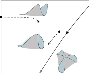
We consider a droplet deposited on a thin elastic sheet, with the contact line pinned at the boundary of the sheet; see figure 1 for an illustration. The droplet–sheet system is surrounded by air. The sheet is very thin in the sense that  $h \ll D$, where $h$ is the thickness of the sheet, and $D$ is its characteristic lateral size. In this model, conceptually we regard the sheet as infinitely thin and identify the sheet with its mid-surface. The parameter $h$ affects only the elastic properties of the sheet.

Figure 1. Schematics of the (a) undeformed and (b) deformed states. Here,  $\varSigma$ is the deformed elastic sheet, $\varGamma$ is the droplet surface, and $\varOmega$ is the 3-D region occupied by the droplet. The unit vectors $\boldsymbol {n}_\varSigma$ and $\boldsymbol {n}_\varGamma$ are the normals of $\varSigma$ and $\varGamma$, respectively; the unit vectors $\boldsymbol {m}_\varSigma$ and $\boldsymbol {m}_\varGamma$ are the co-normals of $\varSigma$ and $\varGamma$ at their boundaries, respectively.
Let  $\varSigma _0$ be the undeformed configuration of the sheet. Let $\varSigma$ be the deformed sheet, with a regular $C^2$ parametrization $\boldsymbol {q} : \varSigma _0 \rightarrow \varSigma$. Denote by $\boldsymbol {n}_\varSigma$ the normal of $\varSigma$, and by $\boldsymbol {m}_\varSigma$ the co-normal at the boundary $\partial \varSigma$. The droplet $\varOmega$ on the sheet has a conserved volume $V$. Let $\varGamma = \partial \varOmega \setminus \varSigma$ be the surface of the droplet in contact with the air, with a regular $C^1$ parametrization $\boldsymbol {r} : \varGamma _0 \rightarrow \varGamma$, where $\varGamma _0$ is the reference domain for the droplet surface. Denote by $\boldsymbol {n}_\varGamma$ its normal, and by $\boldsymbol {m}_\varGamma$ its co-normal at the boundary. Denote by $\varLambda = \partial \varSigma = \partial \varGamma$ the pinned contact line. When no ambiguity arises, we omit the subscripts of $\boldsymbol {n}_{\varSigma }$ and $\boldsymbol {n}_{\varGamma }$.
The total energy of the system reads
 \begin{equation} \mathcal{E} = \mathcal{E}_\varGamma + \mathcal{E}_{\varSigma} + \mathcal{E}_{el}, \end{equation}
where  $\mathcal {E}_{el}$ is the elastic energy of the sheet, and $\mathcal {E}_\varSigma, \mathcal {E}_\varGamma$ are the surface energies of the sheet and the droplet surface, respectively. For the droplet surface, we have
 \begin{equation} \mathcal{E}_\varGamma = \gamma_f \int_\varGamma \mathrm{d} a, \end{equation}
where  $\gamma _f$ is the surface tension coefficient of the fluid–air interface. Similarly, on the elastic sheet, we have
 \begin{equation} \mathcal{E}_\varSigma = \gamma_s \int_\varSigma \mathrm{d} a, \end{equation}
where  $\gamma _s = \gamma _{sf} + \gamma _{sv}$ is the sum of the surface tension coefficients of the fluid–sheet and sheet–air interfaces. Here, we use a two-sided surface energy for the sheet because the contact line is pinned at the sheet boundary. This is in contrast to cases involving a moving contact line, where both surface energies for the wetting and non-wetting regions are relevant and must be considered. Consequently, the classical Young–Dupré relation for the equilibrium contact angle does not apply in our system. Indeed, the equilibrium contact angle at the pinned contact line is not unique and depends on the droplet volume.
We adopt the nonlinear Koiter's shell theory (Koiter Reference Koiter1966; Ciarlet Reference Ciarlet2021) to model the deformations of the elastic sheet. Specifically, the elastic energy can be written as the sum of a stretching part  $\mathcal {E}_s$ and a bending part $\mathcal {E}_b$:
 \begin{equation} \mathcal{E}_{el} = \mathcal{E}_s + \mathcal{E}_b, \end{equation}
where
 $$\begin{gather} \mathcal{E}_s = Y \int_{\varSigma_0} \frac{1}{2}\,\mathcal{A}^{\alpha\beta\gamma\eta} \epsilon_{\alpha\beta} \epsilon_{\gamma\eta} \,\mathrm{d} A, \end{gather}$$
 $$\begin{gather}\mathcal{E}_b = B \int_{\varSigma_0} \frac{1}{2}\,\mathcal{A}^{\alpha\beta\gamma\eta} b_{\alpha\beta} b_{\gamma\eta} \,\mathrm{d} A. \end{gather}$$
Here, the stretching modulus  $Y$ and the bending modulus $B$ are given by
 \begin{equation} Y = \frac{Eh}{1-\nu^2},\quad B = \frac{E h^3}{12(1-\nu^2)}, \end{equation}
where  $E$ is Young's modulus, and $0 \le \nu \le \frac {1}{2}$ is the Poisson ratio. For an isotropic sheet, the fourth-order elastic tensor in (2.5) is given by
 \begin{equation} \mathcal{A}^{\alpha\beta\gamma\eta} = \nu \delta^{\alpha\beta} \delta^{\gamma\eta}+ \tfrac{1}{2} (1 - \nu) (\delta^{\alpha\gamma}\delta^{\beta\eta} + \delta^{\alpha\eta}\delta^{\beta\gamma}), \end{equation}
where  $\delta$ is the Kronecker delta. The stretching strain $\epsilon _{\alpha \beta }$ in (2.5a) is defined as
 \begin{equation} \epsilon_{\alpha\beta} = \tfrac{1}{2}(a_{\alpha\beta} - \delta_{\alpha\beta}), \end{equation}
where  $a_{\alpha \beta } = \partial _\alpha \boldsymbol {q} \boldsymbol {\cdot } \partial _\beta \boldsymbol {q}$ is the first fundamental form of $\varSigma$; see also (A3a). The bending strain $b_{\alpha \beta }$ in (2.5b) is equivalent to the second fundamental form $b_{\alpha \beta } = \partial _\alpha \partial _\beta \boldsymbol {q} \boldsymbol {\cdot } \boldsymbol {n}$ of $\varSigma$; see also (A3b). In (2.5), we used the convention for the summation of repeated indices. All Greek indices such as $\alpha, \beta, \gamma,\eta$ are in $\{1, 2\}$. We will use this convention in the rest of this paper. We note that the area element $\mathrm {d} A$ on the reference domain $\varSigma _0$ is distinguished from its counterpart $\mathrm {d} a$ on the deformed mid-surface $\varSigma$, and similarly for the length elements ${\rm d} L$ and ${\rm d} l$.
2.1. Governing equations
The governing equations for the equilibrium droplet–sheet system can be derived by minimizing the total energy (2.1) subject to the boundary condition
 \begin{equation} \partial \varSigma = \partial \varGamma, \end{equation}
and the constant volume constraint
 \begin{equation} \int_\varOmega \mathrm{d} \kern 0.06em \boldsymbol{x} = V. \end{equation}
Introducing  $p$ as the Lagrange multiplier, we define the Lagrangian
 \begin{equation} \mathcal{L} = \mathcal{E} - p \left( \int_\varOmega \mathrm{d} \kern 0.06em \boldsymbol{x} - V \right). \end{equation}
We then use a variational method to obtain the first-order optimality condition for the equilibrium system. Let  $\delta \boldsymbol {q} : \varSigma _0 \rightarrow \mathbb {R}^3$ be a variation of the sheet, and let $\delta \boldsymbol {r} : \varGamma _0 \rightarrow \mathbb {R}^3$ be a variation of the droplet surface. From the boundary condition (2.9), we note that
 \begin{equation} \delta \boldsymbol{q} = \delta \boldsymbol{r} \quad \text{on } \varLambda. \end{equation}
We introduce the variation operator
 \begin{equation} \delta \mathcal{L} (\boldsymbol{q}, \boldsymbol{r}; \delta \boldsymbol{q}, \delta \boldsymbol{r}) = \left. \frac{\mathrm{d}}{\mathrm{d} \tau} \right|_{\tau = 0} \mathcal{L}(\boldsymbol{q} + \tau\,\delta \boldsymbol{q}, \boldsymbol{r} + \tau\,\delta \boldsymbol{r}), \end{equation}
and write it simply as  $\delta \mathcal {L}$ when no ambiguity arises. The variations of the different energy components are defined similarly.
We compute the variation for each part of the Lagrangian as follows. For the droplet surface energy in (2.2), we have
 \begin{align} \delta \mathcal{E}_\varGamma(\boldsymbol{r}; \delta\boldsymbol{r}) &= \gamma_{f} \int_\varGamma (\boldsymbol{\nabla}_s \boldsymbol{\cdot} \delta \boldsymbol{r}) \,\mathrm{d} a \nonumber\\ &= \int_\varGamma -2\gamma_f H \boldsymbol{n} \boldsymbol{\cdot} \delta \boldsymbol{r} \,\mathrm{d} a + \int_\varLambda \gamma_f \boldsymbol{m}_\varGamma \boldsymbol{\cdot} \delta \boldsymbol{r} \,\mathrm{d} l, \end{align}
where  $\boldsymbol {\nabla }_s\, \boldsymbol {\cdot }$ is the surface divergence operator, and $H=-\frac {1}{2}\boldsymbol {\nabla }_s\boldsymbol {\cdot }\boldsymbol {n}$ is the mean curvature of $\varSigma$. Similarly, for the sheet surface energy in (2.3), we have
 \begin{align} \delta \mathcal{E}_\varSigma(\boldsymbol{q}; \delta\boldsymbol{q}) &= \gamma_s \int_\varSigma (\boldsymbol{\nabla}_s \boldsymbol{\cdot} \delta \boldsymbol{q}) \,\mathrm{d} a \nonumber\\ &= \int_\varSigma -2 \gamma_s H \boldsymbol{n} \boldsymbol{\cdot} \delta \boldsymbol{q} \,\mathrm{d} a + \int_\varLambda \gamma_s \boldsymbol{m}_\varSigma \boldsymbol{\cdot} \delta \boldsymbol{q} \,\mathrm{d} l. \end{align}
For the volume constraint in (2.10), we have
 \begin{equation} \delta \left({-}p \int_\varOmega \mathrm{d} \kern 0.06em \boldsymbol{x} \right) = \int_\varGamma -p \boldsymbol{n} \boldsymbol{\cdot} \delta \boldsymbol{r} \,\mathrm{d} a + \int_\varSigma p \boldsymbol{n} \boldsymbol{\cdot} \delta \boldsymbol{q} \,\mathrm{d} a. \end{equation}
We refer to Walker (Reference Walker2015) for the derivation of these results using shape calculus.
Next, we compute the variation of the elastic energy. To this end, we introduce the second Piola–Kirchhoff stress and moment
 $$\begin{gather} S^{\alpha\beta} = Y \mathcal{A}^{\alpha\beta\gamma\eta} \epsilon_{\gamma\eta}, \end{gather}$$
 $$\begin{gather}M^{\alpha\beta} = B \mathcal{A}^{\alpha\beta\gamma\eta} b_{\gamma\eta}. \end{gather}$$
Then we readily have
 $$\begin{gather} \delta \mathcal{E}_s = \int_{\varSigma_0} S^{\alpha\beta}\,\delta \epsilon_{\alpha\beta} \,\mathrm{d} A, \end{gather}$$
 $$\begin{gather}\delta \mathcal{E}_b = \int_{\varSigma_0} M^{\alpha\beta}\,\delta b_{\alpha\beta} \, \mathrm{d} A. \end{gather}$$
For the stretching strain and the bending strain, it follows from the definition (2.8) and equations (A3a), (A3b) and (A7a) in Appendix A that
 $$\begin{gather} \delta \epsilon_{\alpha\beta} = \tfrac{1}{2} (\partial_\alpha\,\delta \boldsymbol{q} \boldsymbol{\cdot} \partial_\beta\boldsymbol{q} + \partial_\alpha \boldsymbol{q} \boldsymbol{\cdot} \partial_\beta\,\delta \boldsymbol{q}), \end{gather}$$
 $$\begin{gather}\delta b_{\alpha\beta} = \partial_\alpha \partial_\beta\,\delta \boldsymbol{q} \boldsymbol{\cdot} \boldsymbol{n} - \varGamma^{\gamma}_{\alpha\beta} \partial_\gamma\,\delta \boldsymbol{q} \boldsymbol{\cdot} \boldsymbol{n}, \end{gather}$$
where  $\varGamma ^{\gamma }_{\alpha \beta }$ is the Christoffel symbol of the second kind on the sheet $\varSigma$; see (A6). We substitute (2.19) into (2.18), then apply integration by parts and obtain
 \begin{align} \delta \mathcal{E}_s(\boldsymbol{q}; \delta \boldsymbol{q}) &= \int_{\partial \varSigma_0} S^{\alpha\beta} N_\beta (\partial_\alpha \boldsymbol{q} \boldsymbol{\cdot} \delta \boldsymbol{q})\,\mathrm{d} L \nonumber\\ &\quad +\int_{\varSigma_0} - \boldsymbol{\nabla}_\beta S^{\alpha\beta} (\partial_\alpha \boldsymbol{q} \boldsymbol{\cdot} \delta \boldsymbol{q}) - S^{\alpha\beta} b_{\alpha\beta} (\boldsymbol{n} \boldsymbol{\cdot} \delta \boldsymbol{q})\,\mathrm{d} A, \end{align}
 \begin{align} \delta \mathcal{E}_b(\boldsymbol{q}; \delta \boldsymbol{q}) &= \int_{\partial \varSigma_0} -\left\{\boldsymbol{\nabla}_\beta M^{\alpha\beta} N_\alpha + \frac{\partial}{\partial \boldsymbol{L}} (M^{\alpha\beta} L_\alpha N_\beta)\right\} (\boldsymbol{n} \boldsymbol{\cdot} \delta \boldsymbol{q}) \nonumber\\ &\quad + 2 b^{\alpha}_{\eta} M^{\eta\beta} N_\beta (\partial_\alpha \boldsymbol{q} \boldsymbol{\cdot} \delta \boldsymbol{q})+ M^{\alpha\beta} N_\alpha N_\beta\, \frac{\partial}{\partial \boldsymbol{N}} (\boldsymbol{n} \boldsymbol{\cdot} \delta \boldsymbol{q})\,\mathrm{d} L \nonumber\\ &\quad + \int_{\varSigma_0}(\boldsymbol{\nabla}_{\alpha} \boldsymbol{\nabla}_{\beta} M^{\alpha\beta} - M^{\alpha\beta} c_{\alpha\beta})(\boldsymbol{n} \boldsymbol{\cdot} \delta \boldsymbol{q}) \nonumber\\ &\quad - \{\boldsymbol{\nabla}_\beta (b^{\alpha}_{\eta} M^{\eta\beta}) + b^{\alpha}_{\eta}\,\boldsymbol{\nabla}_\beta M^{\eta\beta}\} (\partial_\alpha \boldsymbol{q} \boldsymbol{\cdot} \delta \boldsymbol{q})\,\mathrm{d} A, \end{align}
where  $\boldsymbol {L} = (L_1, L_2)$ and $\boldsymbol {N} = (N_1, N_2)$ are the unit tangent and normal vectors of $\partial \varSigma _0$, respectively, $b_\eta ^\alpha$ is defined in (A4a,b), and $c_{\alpha \beta }$ is the third fundamental form of the sheet $\varSigma$; see (A3c). The covariant derivatives are defined as
 $$\begin{gather} \boldsymbol{\nabla}_\beta V^{\beta} = \partial_\beta V^{\beta}, \end{gather}$$
 $$\begin{gather}\boldsymbol{\nabla}_\beta M^{\alpha\beta} = \partial_\beta M^{\alpha\beta} + \varGamma^{\alpha}_{\beta\gamma} M^{\beta\gamma}, \end{gather}$$
for a first-order tensor  $V^{\beta }$ and a second-order tensor $M^{\alpha \beta }$, respectively.
We then combine (2.14)–(2.16) and (2.20), and require  $\delta \mathcal {L}$ to vanish for all smooth variations $\delta \boldsymbol {q}$ and $\delta \boldsymbol {r}$. This leads to the governing equations for the equilibrium system as follows.
(i) On the droplet surface, we have the usual Laplace equation
(2.22)The droplet surface thus has a constant mean curvature. The Lagrange multiplier \begin{equation} -\!2 \gamma_f H - p = 0 \quad \text{on } \varGamma. \end{equation}$p$, which plays the role of pressure, determines the mean curvature.
(ii) On the undeformed sheet (or reference domain)
$\varSigma _0$, we have
(2.23a)$$\begin{gather} \boldsymbol{\nabla}_\alpha \boldsymbol{\nabla}_\beta M^{\alpha\beta} - M^{\alpha\beta} c_{\alpha\beta} - S^{\alpha\beta} b_{\alpha\beta}= \frac{\mathrm{d} a}{\mathrm{d} A}\,(2 \gamma_s H + p), \end{gather}$$(2.23b)where$$\begin{gather}-\boldsymbol{\nabla}_\beta (S^{\alpha\beta} + b^{\alpha}_{\eta} M^{\eta\beta}) - b^{\alpha}_{\eta}\, \boldsymbol{\nabla}_{\beta} M^{\eta\beta} = 0, \quad \alpha = 1, 2, \end{gather}$$$\mathrm {d} a / \mathrm {d} A$ is the ratio between the deformed and undeformed area elements. Here, (2.23a) states the balance of the elastic force (the left-hand side), the curvature force and the fluid pressure (the right-hand side) in the direction normal to the sheet; (2.23b) states the balance of elastic forces in the tangential directions.(iii) Along the boundary
$\partial \varSigma _0$ of the reference domain, we have
(2.24a)$$\begin{gather} M^{\alpha\beta} N_\alpha N_\beta = 0, \end{gather}$$(2.24b)$$\begin{gather}-\boldsymbol{\nabla}_\beta M^{\alpha\beta} N_\alpha - \frac{\partial}{\partial \boldsymbol{L}} (M^{\alpha\beta} L_\alpha N_\beta)= \frac{\mathrm{d} l}{\mathrm{d} L}\,\boldsymbol{f} \boldsymbol{\cdot} \boldsymbol{n}_{\varSigma}, \end{gather}$$(2.24c)where$$\begin{gather}(S^{\alpha\beta} + 2 b^{\alpha}_{\eta} M^{\eta\beta}) N_\beta = \frac{\mathrm{d} l}{\mathrm{d} L}\,\boldsymbol{f} \boldsymbol{\cdot} \boldsymbol{q}^{(\alpha)}, \quad \alpha = 1, 2, \end{gather}$$$\mathrm {d} l / \mathrm {d} L$ is the ratio between the deformed and undeformed arc-length elements along $\partial \varSigma _0$, $\{\boldsymbol {q}^{(\alpha )}: \alpha =1, 2\}$ is the dual basis of the tangent space of the sheet (see (A2)), and $\boldsymbol {f}$ is the combination of the surface tension forces given by
(2.25)Here, (2.24a) is the moment-free condition; (2.24b) and (2.24c) state the balance of the elastic force (the left-hand side) and the surface tension forces (the right-hand side) in the normal and tangential directions, respectively.\begin{equation} \boldsymbol{f} ={-} \gamma_f \boldsymbol{m}_{\varGamma} - \gamma_s \boldsymbol{m}_{\varSigma}. \end{equation}


2.2. Non-dimensionalization
Equations (2.22)–(2.24) with the boundary condition (2.9) and the constant volume constraint (2.10) form the governing equations for the equilibrium system. We make the system dimensionless by using  $D$ as the characteristic length and $\gamma _f D^2$ as the characteristic energy. The physical parameters are transformed as
 \begin{equation} \tilde{\gamma}_f = 1,\quad \tilde{\gamma}_s = \frac{\gamma_s}{\gamma_f},\quad \tilde{Y} = \frac{Y}{\gamma_f},\quad \tilde{B}= \frac{B}{\gamma_f D^2}. \end{equation}
The variables are rescaled accordingly, e.g.
 \begin{align} \tilde{\boldsymbol{q}} = \frac{\boldsymbol{q}}{D}, \quad \tilde{\epsilon}_{\alpha\beta} = \epsilon_{\alpha\beta}, \quad \tilde{S}^{\alpha\beta} = \tilde{Y} \mathcal{A}^{\alpha\beta\gamma\eta} \tilde{\epsilon}_{\gamma\eta}, \quad \tilde{b}_{\alpha\beta} = D b_{\alpha\beta}, \quad \tilde{M}^{\alpha\beta} = \tilde{B} \mathcal{A}^{\alpha\beta\gamma\eta} \tilde{b}_{\gamma\eta}, \end{align}
and so on. Note that  $\tilde {Y}/\tilde {B} = 12 (D/h)^2 \gg 1$ for thin sheets. In view of the capillary-bending length $l_{B} = ( B / \gamma _f )^{1/2}$, the dimensionless bending modulus can be written as
 \begin{equation} \tilde{B} = ({l_{B}}/{D})^{2}. \end{equation}
Thus  $\tilde {B}^{1/2}$ is the ratio between the capillary-bending length and the sheet size. For sufficiently small $\tilde {B}$, the capillary force is then strong enough to fold the sheet into a 3-D structure. In the literature, the critical bendability $B_{{crit}}$ is the bendability below which a folded structure can be attained upon evaporation of the droplet.
Hereafter, we will use the dimensionless equations and drop the overhead tildes for the sake of simplicity.
2.3. Relaxation dynamics
We consider a relaxation dynamics of the droplet–sheet system in which the total energy decays over time. Following this dynamics, the system reaches equilibrium at the steady state. We focus on systems where the relaxation time scale of the droplet is much faster than that of the sheet. We therefore assume that the droplet is in a quasi-static state during the relaxation process. In other words, at every instant  $t$, given the sheet $\varSigma (t)$ with the parametrization $\boldsymbol {q}(t, {\cdot }\,)$, the droplet surface $\varGamma (t)$ is determined via
 \begin{equation} -\!2 H_{\varGamma(t)} - p(t) = 0, \end{equation}
subject to the boundary condition
 \begin{equation} \partial \varSigma(t) = \partial \varGamma(t), \end{equation}
and the constraint
 \begin{equation} \int_{\varOmega(t)} \mathrm{d} \kern 0.06em \boldsymbol{x} = V, \end{equation}
where  $\varOmega (t)$ is the region enclosed by $\varSigma (t)$ and $\varGamma (t)$. Based on (2.23), we consider the relaxation dynamics of the sheet governed by
 \begin{align} \frac{\partial \boldsymbol{q}}{\partial t} &= \left\{ -\boldsymbol{\nabla}_\alpha \boldsymbol{\nabla}_\beta M^{\alpha\beta} + M^{\alpha\beta}c_{\alpha\beta} + S^{\alpha\beta}b_{\alpha\beta}+ \frac{\mathrm{d} a}{\mathrm{d} A}\,( 2 \gamma_s H_{\varSigma} + p) \right\} \boldsymbol{n}_{\varSigma} \nonumber\\ &\quad + \{\boldsymbol{\nabla}_\beta( S^{\alpha\beta} + b^\alpha_\eta M^{\eta\beta}) + b^\alpha_\eta\,\boldsymbol{\nabla}_\beta M^{\eta\beta}\}\,\partial_a \boldsymbol{q}, \end{align}
where the two terms on the right-hand side are the relaxation of the sheet in the normal and tangential directions, respectively. In general, we may introduce additional parameters to control the time scale of relaxation in different directions; however, for the sake of simplicity, we consider the relaxation dynamics as given above since our main focus is the equilibrium state. The dynamics (2.32) is subject to the boundary conditions
 $$\begin{gather} M^{\alpha\beta} N_\alpha N_\beta = 0, \end{gather}$$
 $$\begin{gather}-\boldsymbol{\nabla}_\beta M^{\alpha\beta} N_\alpha - \frac{\partial}{\partial \boldsymbol{L}} (M^{\alpha\beta} L_\alpha N_\beta)= \frac{\mathrm{d} l}{\mathrm{d} L}\,\boldsymbol{f}(t) \boldsymbol{\cdot} \boldsymbol{n}_{\varSigma}, \end{gather}$$
 $$\begin{gather}(S^{\alpha\beta} + 2 b^{\alpha}_{\eta} M^{\eta\beta}) N_\beta = \frac{\mathrm{d} l}{\mathrm{d} L}\,\boldsymbol{f}(t) \boldsymbol{\cdot}\boldsymbol{q}^{(\alpha)}, \quad \alpha = 1, 2, \end{gather}$$
where
 \begin{equation} \boldsymbol{f}(t) ={-}\boldsymbol{m}_{\varGamma(t)} - \gamma_s \boldsymbol{m}_{\varSigma(t)}. \end{equation}
Note that in this system,  $S^{\alpha \beta }$, $M^{\alpha \beta }$ and $\boldsymbol {\nabla }_{\alpha }$ depend on $t$ as they are functions of $\boldsymbol {q}(t, {\cdot }\,)$.
3. Numerical method
In this section, we give a brief description of the numerical method for solving the relaxation dynamics (2.29)–(2.33). The implementation details will be reported in another paper. A validation of the accuracy and robustness of this method is provided in Appendix C.
We first review briefly some related earlier work. Several numerical methods have been proposed in the literature for systems involving fluid–membrane interactions, among which are the immersed boundary method (Lai & Ong Reference Lai and Ong2019) and the parametric finite element method (Barrett, Garcke & Nürnberg Reference Barrett, Garcke and Nürnberg2017). For modelling biomembranes with the Willmore energy, the phase field method (Du, Liu & Wang Reference Du, Liu and Wang2004) and the discrete differential geometry method (Seol et al. Reference Seol, Hu, Kim and Lai2016) have been employed. For the simulation of nonlinear Koiter's sheets or shells, there exist lattice-based methods (Chen & Zhang Reference Chen and Zhang2022), the finite difference method (Alben et al. Reference Alben, Gorodetsky, Kim and Deegan2019), the Hermite finite element method (Heil & White Reference Heil and White2002), and the non-uniform rational basis spline based isogeometric analysis (Kiendl et al. Reference Kiendl, Bletzinger, Linhard and Wüchner2009).
In our method, we reformulate the dynamical equation (2.32) into a weak form. We find the sheet  $\boldsymbol {q}(t, {\cdot }\,)$ such that for $t \ge 0$ and all test functions $\boldsymbol {\psi }$, the following equation holds:
 \begin{align} \int_{\varSigma_0} \frac{\partial \boldsymbol{q}}{\partial t} \boldsymbol{\cdot} \boldsymbol{\psi} \,\mathrm{d} A &={-} \delta \mathcal{E}_{el}(\boldsymbol{q}; \boldsymbol{\psi})- \delta \mathcal{E}_{\varSigma} (\boldsymbol{q}; \boldsymbol{\psi}) \nonumber\\ &\quad - \int_{\varSigma(t)} p(t)\,\boldsymbol{n}_{\varSigma(t)} \boldsymbol{\cdot} (\boldsymbol{\psi}\circ\boldsymbol{q}^{{-}1}) \,\mathrm{d} a \nonumber\\ &\quad - \int_{\varLambda(t)} \boldsymbol{m}_{\varGamma(t)} \boldsymbol{\cdot} (\boldsymbol{\psi}\circ\boldsymbol{q}^{{-}1}) \, \mathrm{d} l, \end{align}
where  $\varSigma (t) = \operatorname {Im}\boldsymbol {q}(t)$, $\varLambda (t) = \partial \varSigma (t)$, and $\varGamma (t)$ is the surface of constant mean curvature determined by (2.29)–(2.31).
Let  $\Delta t$ be the time step, and let $\boldsymbol {q}^m$ be the numerical approximation to the sheet at $t = m\Delta t$. At each time step, with the sheet $\varSigma ^m = \operatorname {Im}\boldsymbol {q}^m$ given, we first determine the droplet surface $\varGamma ^m$ and the Laplace pressure $p^m$ that satisfy the following equations:
 $$\begin{gather} -2H - p^m = 0 \quad \text{on } \varGamma^m, \end{gather}$$
 $$\begin{gather}\partial \varGamma^m = \partial \varSigma^m, \end{gather}$$
 $$\begin{gather}\int_{\varOmega^m} \mathrm{d} \kern 0.06em \boldsymbol{x} = V. \end{gather}$$
Following this, we proceed to update the elastic sheet and compute  $\boldsymbol {q}^{m+1}$. For stability considerations, we use a semi-implicit scheme to discretize (3.1). In this scheme, the elastic force and the curvature force on the right-hand side of the equation are treated implicitly, while the coupling with the droplet is treated explicitly. This leads to the following semi-discrete scheme: for all test functions $\boldsymbol {\psi }$,
 \begin{align} \int_{\varSigma_0} \frac{\boldsymbol{q}^{m+1} - \boldsymbol{q}^m}{\Delta t} \boldsymbol{\cdot} \boldsymbol{\psi} \,\mathrm{d} A &={-} \delta \mathcal{E}_{el}(\boldsymbol{q}^{m+1}; \boldsymbol{\psi}) - \delta \mathcal{E}_{\varSigma} (\boldsymbol{q}^{m+1}; \boldsymbol{\psi}) \nonumber\\ &\quad - \int_{\varSigma^m} p^m \boldsymbol{n}_{\varSigma^m} \boldsymbol{\cdot} (\boldsymbol{\psi}\circ(\boldsymbol{q}^m)^{{-}1})\,\mathrm{d} a \nonumber\\ &\quad - \int_{\varLambda^m} \boldsymbol{m}_{\varGamma^m} \boldsymbol{\cdot} (\boldsymbol{\psi}\circ(\boldsymbol{q}^m)^{{-}1})\,\mathrm{d} l, \end{align}
where  $\varLambda ^m = \partial \varSigma ^m$.
Next, we consider spatial discretizations of the elastic sheet and the droplet surface. In view of the second-order derivatives in the nonlinear Koiter's energy, the discrete function space for  $\boldsymbol {q}$ is required to have square-integrable second-order derivatives. This can be achieved by using a finite element space with $C^1$ continuity. Here, we employ the subdivision element method, which provides $C^1$ conforming basis functions on unstructured triangular meshes. These basis functions are implicitly defined through the Loop's subdivision procedure (Loop Reference Loop1987). The subdivision element method was first introduced in Cirak et al. (Reference Cirak, Ortiz and Schröder2000) and Cirak & Ortiz (Reference Cirak and Ortiz2001) for analysing thin elastic shells. It was later employed in Feng & Klug (Reference Feng and Klug2006) and Chen et al. (Reference Chen, Yu, Brogan, Kusner, Yang and Zigerelli2020) to study deformations of biomembranes.
The governing equations for the droplet surface  $\varGamma ^m$ in (3.2) are solved by using a Ritz method. To be specific, let $\boldsymbol {r}: \varGamma _0 \rightarrow \mathbb {R}^3$ be a parametrization of a droplet surface. Consider the following functional:
 \begin{equation} \mathcal{A}[\boldsymbol{r}] =\frac{1}{2} \int_{\varGamma_0} J(\boldsymbol{r})^2\,\mathrm{d} a, \end{equation}
where  $\varGamma = \operatorname {Im}\boldsymbol {r}$ satisfies the boundary condition (3.2b) and the constant volume constraint (3.2c), and $J(\boldsymbol {r})$ is the area Jacobian between $\varGamma$ and $\varGamma _0$. It was shown (Renka Reference Renka2015) that the minimizer of the above functional gives a surface with constant mean curvature. Moreover, this approach selects a specific parametrization for the constant mean curvature surface that preserves mesh quality, in the sense that the area Jacobian $J(\boldsymbol {r})$ is constant on the surface. The functional (3.4) is discretized using piecewise linear finite elements and subsequently minimized using the MATLAB routine fmincon.
We summarize the overall algorithm as follows. Initially, we are given the elastic sheet  $\boldsymbol {q}^0$, and the droplet volume $V$. For each time step $m\ge 0$, we do the following.
(1) Determine the droplet surface
$\varGamma ^{m}$ by minimizing the functional (3.4) subject to the boundary condition (3.2b) and the constraint (3.2c).(2) Update the elastic sheet. Find
$\boldsymbol {q}^{m+1} \in \mathcal {S}_{{sbdv}}$ such that (3.3) holds for all test functions $\boldsymbol {\psi } \in \mathcal {S}_{{sbdv}}$, where $\mathcal {S}_{{sbdv}}$ is the subdivision element space. The resulting nonlinear system about $\boldsymbol {q}^{m+1}$ is solved by Newton's method.


We repeat these two steps until the system reaches the equilibrium state.
During long-time simulations, the system may undergo large deformations, resulting in significant mesh distortion on the droplet surface. This can lead to ill-conditioned systems and slow down the convergence of the optimization routine. To maintain a high-quality mesh, we incorporate a re-meshing step into the algorithm: We perform re-meshing on  $\varGamma ^m$ using the software JIGSAW (Engwirda & Ivers Reference Engwirda and Ivers2016) whenever the deformation gradient is $\Vert \boldsymbol {\nabla } \boldsymbol {r}^m \Vert _{L^\infty } \ge 1.6$. At the same time, we set the current droplet surface $\varGamma ^m$ as the new reference domain $\varGamma _0$ for subsequent computations. The effect of re-meshing is illustrated in figure 2.

Figure 2. Mesh on the droplet surface in the example of a triangular sheet (see § 4.1). (a) No re-meshing is performed throughout the simulation. (b) Re-meshing is performed, and  $\varGamma _0: = \varGamma ^m$ whenever $\Vert \boldsymbol {\nabla } \boldsymbol {r}^m \Vert _{L^\infty } \ge 1.6$. (c) Aspect ratio of the triangles in meshes (a,b). The aspect ratio is calculated as the ratio between the longest and shortest edges of each triangle.
4. Results and discussions
We consider a polydimethylsiloxane (PDMS) sheet of thickness  $h = 40\,\mathrm {\mu }$m, the Poisson ratio $\nu = 1/2$, and the Young's modulus $E = 7.5 \times 10^5$ Pa. The diameter of the sheet is taken to be 2 mm. At room temperature, the surface tension coefficients are $\gamma _f = 7.5 \times 10^{-2}$ and $\gamma _s = 2 \times 10^{-2}$ N m $^{-1}$. The dimensionless parameters are calculated to be
 \begin{equation} Y = 5.33 \times 10^2, \quad B = 1.78 \times 10^{{-}2}, \quad \gamma_s = 2.67 \times 10^{{-}1}. \end{equation}
Numerical simulations presented below are conducted under these parameters unless stated otherwise.
4.1. Relaxation process
In this subsection, we present the relaxation process of the droplet–sheet system towards the equilibrium state. We assume that the evaporation time scale is much slower than the relaxation time scale. Therefore, we fix the droplet volume in the following examples.
4.1.1. Triangular sheets
First, we study the folding of a triangular sheet. The sheet is in the shape of an equilateral triangle with side length  $D = 1$. The sharp corners of the triangle require a fine mesh in the discretization. To optimize computational efficiency, we mitigate this by using circular arcs with radius $0.05$ to round the corners. Our numerical results (not shown) demonstrate that rounding out the corners has little effect on the folded structures. Initially, a droplet of volume $V = 0.074$ is placed on top of the sheet. The system is then allowed to relax with the droplet volume fixed. Four states during the relaxation process are presented in figure 3. We observe that the three corners of the sheet are gradually pulled up by the capillary force. Throughout the process, the system remains threefold symmetric. After reaching equilibrium, the sheet partially wraps up the droplet. The mesh on the droplet surface is shown in figure 2(b). From this equilibrium state, we may further decrease the droplet volume to obtain a completely folded state.

Figure 3. Folding of a triangular sheet by capillary force. The droplet has fixed volume  $V = 0.074$. (a–d) Snapshots of the folding process. The insets are top views of the droplet–sheet system. (e) Changes of the various energy components following the relaxation dynamics. See also supplementary movie 1, available at https://doi.org/10.1017/jfm.2023.1051.
4.1.2. Square sheets
Next, we present the folding process for a square sheet. The sheet has side length  $D=1$, with the corners rounded by circular arcs of radius $0.1$. Initially, a droplet of volume $V = 0.25$ is placed on the sheet. The system is then allowed to relax with the droplet volume fixed. The change of energies in figure 4(e) shows that the relaxation process consists of three stages. In the first stage, the edges of the square sheet are pulled up by the capillary force; see figure 4(b). This stage soon transitions to the next: the corners of the sheet are pulled up, while the edges are released; see figure 4(c). By now, the sheet remains fourfold symmetric. As the system continues to relax, it reaches the final equilibrium state with twofold symmetry; see figure 4(d).

Figure 4. Folding of a square sheet by capillary force. The droplet has fixed volume  $V = 0.25$. (a–d) Snapshots of the folding process. The insets are top views of the droplet–sheet system. (e) Changes of the various energy components following the relaxation dynamics. See also supplementary movie 2.
The numerical results show that the energy gradients (i.e. the right-hand side of (2.32)) at the intermediate states in figures 4(b,c) are extremely small. This can also be observed from the plot of the total energy, which is rather flat in these states. However, we cannot ascertain whether these states are indeed critical points of the energy functional. Further mathematical analysis is needed to characterize the nature of these states.
4.1.3. Cubic encapsulation
Next, we simulate the cubic encapsulation of a droplet. In its initial undeformed state, the sheet is the expansion of the surface of a cube with side length  $D/4 = 1/4$. The sharp corners are rounded by circular arcs of radius $0.1$. Initially, as shown in figure 5(a), a droplet with volume $V = 0.078$ is placed onto the sheet. As the system relaxes, the panels of the sheet are bent towards the droplet by the capillary force. Since the droplet volume is far larger than the encapsulation volume (i.e. the volume of the cube), the sheet only partially wraps the droplet at equilibrium.

Figure 5. Dynamics of the cubic encapsulation, with fixed droplet volume  $V = 0.078$. (a–d) Snapshots of the folding process. The insets are top views of the droplet–sheet system. (e) Changes of the various energy components following the relaxation dynamics. See also supplementary movie 3.
4.1.4. Spherical encapsulation
In the last example, we simulate the spherical encapsulation of a droplet. In its undeformed state, the sheet takes the shape of a flower with six petals; see Appendix D for the MATLAB code to generate the shape. Here,  $D=1$ is the distance between the tips of opposite petals. Initially, a droplet of volume $V = 0.03$ is placed onto the sheet. In figures 6(a–d), we show the relaxation process of the spherical encapsulation. During this process, the petals of the sheet are first being pulled upward by the capillary force, until they reach an upright position. After that, the petals are being pulled towards the centre so as to form a spherical encapsulation at equilibrium.

Figure 6. Dynamics of the spherical encapsulation of a droplet with fixed volume  $V = 0.03$. (a–d) Snapshots of the folding process. The insets are top views of the droplet–sheet system.
4.2. Folded structures at equilibrium
To demonstrate further the capability of the proposed model, we vary the droplet volume, examine the folded structures at equilibrium, and compare the results with the experimental findings presented in Py et al. (Reference Py, Reverdy, Doppler, Bico, Roman and Baroud2007).
(i) For a triangular sheet, we simulate the relaxation dynamics with a slowly decreasing droplet volume. The rate of the volume decrease is slow, so at each instant, the system is approximately at equilibrium; see supplementary movie 4 for the simulated process. Two equilibrium configurations are shown in figures 7(a) and 7(b), corresponding to droplet volumes
$V = 0.074$ and $V = 0.037$, respectively. In the latter case, we obtain a folded state where the corners of the triangular sheet are about to make contact. Further decreasing the volume will result in a ‘pyramid’ encapsulation, as depicted in figure 1(b) of Py et al. (Reference Py, Reverdy, Doppler, Bico, Roman and Baroud2007). However, we note that capturing the self-contacts of the sheet is beyond the capability of our numerical method.(ii) For a square sheet, the state with fourfold symmetry remains stable when the droplet is large. However, as the droplet volume is decreased below
$V = 0.5$, the fourfold symmetric state gradually loses stability, and the system transitions to centreline folding characterized by twofold symmetry; see figures 8(a) and 8(b). As the volume is decreased further, the sheet tends to wrap the droplet in a quasi-cylindrical shape. At $V = 0.112$, the pairs of adjacent corners are about to touch, dividing the droplet surface into three pieces, with an oval shape at the top, as shown in figure 8(c). We refer to supplementary movie 5 for the evaporation process.In the experiments of Guo et al. (Reference Guo, Li, Yeop Ahn, Duoss, Hsia, Lewis and Nuzzo2009) and Py et al. (Reference Py, Reverdy, Doppler, Bico, Roman and Baroud2007), they observed a diagonal folding state when two opposite corners of the square sheet are significantly rounded. We observed a similar phenomenon in our simulation: by replacing a pair of opposite corners with circular arcs of radius
$0.2$, we obtained a diagonal folding state as shown in figure 8(d). However, as the droplet volume falls below a certain threshold, the diagonal folding state disappears, and the system transitions to a centreline folding state.(iii) For cubic encapsulation, we start with the configuration in figure 5(d), and gradually decrease the droplet volume. The equilibrium state corresponding to the volume
$V = 0.029$ is shown in figure 9(a), where the panels of the sheet nearly form the surface of a cube.(iv) For spherical encapsulation, we present the configuration shown earlier (in figure 6d) in a different view in figure 9(b) and make a comparison with the experimental result.


Figure 7. (a,b) Equilibrium states of the droplet–triangular sheet system with two different droplet volumes, and (c,d) a comparison with the experimental results (Py et al. Reference Py, Reverdy, Doppler, Bico, Roman and Baroud2007).

Figure 8. (a–d) Equilibrium states of the droplet–square sheet system with different droplet volumes, and (e–h) a comparison with the experimental results (Py et al. Reference Py, Reverdy, Doppler, Bico, Roman and Baroud2007).

Figure 9. Equilibrium states of (a) cubic encapsulation and (b) spherical encapsulation, and (c,d) a comparison with the experimental results (Py et al. Reference Py, Reverdy, Doppler, Bico, Roman and Baroud2007).
We conclude that very good qualitative agreement is observed between the simulation and the experimental results.
4.3. Bifurcation diagrams
We now focus on triangular sheets and study their folding behaviours under different bendabilities ( $B$), while keeping $Y = 5.33 \times 10^2$ and $\gamma _s = 2.67 \times 10^{-2}$ fixed. In previous 2-D models, a critical bendability $B^\ast$ was identified. Upon evaporation of the droplet, the sheet unfolds when $B > B^\ast$, and wraps up when $B < B^\ast$. Our 3-D model shows richer behaviours. We observe that a triangular sheet can fold in either a mode-2 or a mode-3 manner. In mode-2 folding, two vertices of the sheet are pulled up by the capillary force, resulting in a state symmetric about the centreline of the triangular sheet. Moreover, for a given droplet volume, equilibrium states with both large and small droplet surface areas can co-exist. Typical configurations of these states are shown in figures 10(a) and 10(b). We will refer to these states as mode-2(a) and mode-2(b), respectively. In contrast, mode-3 folding exhibits threefold symmetry, with all three vertices being pulled up and tending to attach to each other, as shown in figure 10(c).

Figure 10. Typical configurations of (a,b) mode-2 folding,  $B=0.04$, $V=0.037$, and (c) mode-3 folding, $B=0.04$, $V=0.074$, of a triangular sheet.
Following the typical experimental set-up, we study the equilibrium states attained through droplet evaporation. The evaporation rate is slow, allowing the system to reach an equilibrium state at each instant. When the bendability is large, the sheet eventually becomes flat as the droplet evaporates fully. When the bendability is small, the sheet adopts a mode-3 folded state during the evaporation of the droplet. In cases of intermediate bendabilities, the sheet takes on a mode-2 folded state upon droplet evaporation. Accordingly, we classify the folding of triangular sheets into three regimes, as described below.
In Regime I, an unfolded state is attained eventually. Initially, when the droplet volume is large, the system exhibits threefold symmetry and adopts a mode-3 configuration. This equilibrium state disappears when the volume is below a certain value. The system then transitions to a twofold symmetry and takes on a mode-2(a) state. Eventually, the sheet becomes flat as the droplet evaporates fully. A typical path that the system follows is shown in figure 11. The mode-2(a) and mode-2(b) states co-exist within a certain range of droplet volumes. However, the mode-2(b) folding state is not realized in this evaporation process.

Figure 11. Bifurcation diagram in Regime I. The sheet bendability is  $B = 0.048$. (a) The rescaled area of the droplet surface versus the rescaled droplet volume. (b) The total energy $\mathcal {E}$ versus the rescaled volume. Here, $V_{{encap}} = 1/48 \sqrt {2}$ is the volume of the tetrahedron that can be formed by the triangular sheet, and $|\varSigma _0|$ is the area of the undeformed sheet. In both plots, the ends of the branches for mode-2(a), mode-2(b) and mode-3 states are marked by $\blacksquare, \blacklozenge$ and $\bullet$, respectively. Solid lines are the paths that the system follows as the droplet volume is decreased.
In Regime II, a mode-2(b) folded state is attained eventually. The system exhibits threefold symmetry when the droplet volume is large, and transitions to a twofold symmetry when the volume is below a certain value. As the volume is decreased further, a mode-2(b) folded state is attained. A typical path that the system follows is shown in figure 12. Again, the mode-2(a) and mode-2(b) states co-exist within a certain range of the droplet volume, but the mode-2(a) state is not realized in the evaporation process.

Figure 12. Bifurcation diagram in Regime II. The sheet bendability is  $B = 0.040$. (a) The rescaled area of the droplet surface versus the rescaled droplet volume. (b) The system energy $\mathcal {E}$ versus the rescaled volume. See the caption of figure 11 for descriptions of the symbols.
In Regime III, a mode-3 folded state is attained eventually. The system maintains threefold symmetry throughout the evaporation process. A typical path that the system follows is shown in figure 13. Neither mode-2(a) nor mode-2(b) states are realized in the evaporation process.

Figure 13. Bifurcation diagram in Regime III. The sheet bendability is  $B = 0.030$. (a) The rescaled area of the droplet surface versus the rescaled droplet volume. (b) The system energy $\mathcal {E}$ versus the rescaled volume. See the caption of figure 11 for descriptions of the symbols.
From the bifurcation diagrams, we see that multiple equilibrium states can co-exist. As a result, the system exhibits hysteretic effects. This phenomenon is indeed observed in the simulations. Taking Regime II (see figure 12) as an example, when the droplet volume is decreased gradually, the system assumes the mode-2(b) folding state within the volume range  $V \lesssim 3.7 V_{{encap}}$; in contrast, when the droplet volume is increased gradually from $V=0$ up to approximately $3 V_{{encap}}$, the system adopts the mode-2(a) state (results not shown).
We also note that the dynamical process discussed above depends on the rate of volume change. The bifurcation diagrams show the paths that the system follows when the droplet volume is decreased at a very slow rate, allowing the system to reach equilibrium at each moment. However, at a faster rate, the dynamics of the system may deviate from those paths. Taking Regime II as an example again, when the volume is decreased at rate  $\mathrm {d} V / \mathrm {d} t = 0.0184$, the system adopts the mode-2(a) state and follows the mode-2(a) branch after leaving the mode-3 branch. In this case, the system eventually assumes a flat configuration upon complete droplet evaporation.
4.4. Critical bendability
We proceed to identify the critical bendabilities for both square and triangular sheets. The critical bendability, denoted by  $B_{{crit}}$, is defined as the bendability below which a mode-2 folding (for square sheets) or a mode-3 folding (for triangular sheets) occurs upon complete droplet evaporation. Numerical results for these critical values are shown in figure 14.

Figure 14. The critical bendabilities  $B_{{crit}}$ for different stretching modulus $Y$. The upper line corresponds to the mode-2 folding of a square sheet, and the lower line corresponds to the mode-3 folding of a triangular sheet.
We make two observations from the numerical results. First, under the same stretching modulus, the critical bendability is higher for the mode-2 folding of a square sheet than for the mode-3 folding of a triangular sheet. In other words, it is easier to fold a square sheet than a triangular sheet of the same size. This observation agrees with the experimental results of Py et al. (Reference Py, Reverdy, Doppler, Bico, Roman and Baroud2007). Second, the critical bendabilities decrease as the stretching modulus increases. While these values exhibit minor changes for a square sheet, they decrease considerably for a triangular sheet. This observation is absent from previous 2-D studies and reveals the interplay between the stretching and bending of the sheet when wrapping a droplet in three dimensions.
We also note the connection between our results and those in Py et al. (Reference Py, Reverdy, Doppler, Bico, Roman and Baroud2007). There, they assumed a linear relation between  $l_{{crit}}$ and $l_B$, where $l_{{crit}}$ is the sheet's critical folding length, and $l_B$ is the capillary-bending length, and reported the ratio $\alpha = l_{{crit}} / l_B$ by linear regression on the measured data. In view of the definition of the dimensionless bendability in (2.28), we see that this ratio is related to the critical bendability via
 \begin{equation} B_{{crit}} = \left( \frac{l_B}{l_{{crit}}}\right)^2 = \alpha^{{-}2}. \end{equation}
Thus  $B_{{crit}} \approx 0.021$ for the mode-2 folding of a square sheet, and $B_{{crit}} \approx 0.0069$ for the mode-3 folding of a triangular sheet, according to the experimental results. These values are smaller than those that we obtained in our simulations. Such a discrepancy might be caused partially by the mismatch of parameters. Another possible reason is that their $(l_{{crit}}, l_B)$ data were measured for systems with varying stretching modulus $Y$. To our understanding, in their measurements, $l_B$ was altered by modifying the sheet's thickness, which could consequently alter its stretching modulus. Thus the result from linear regression on such data might not be comparable directly to the critical bendability obtained in our simulations, given the latter's dependence on the stretching modulus.
5. Conclusion
In this work, we introduced a mathematical model for the capillary folding of thin elastic sheets in three dimensions. We began with the system free energy that consists of interfacial energies and the nonlinear Koiter's energy for the elastic sheet. The employment of the Koiter's energy allowed us to study large deformations of the sheet in three dimensions. This is in contrast to simplified 1-D or 2-D models used in previous work, such as the Euler's elastica for beams and the FvK model for plates with small deflections.
We derived the governing equations for the equilibrium system by a variational method. On the thin sheet, we obtained Koiter's equations, which give the balance between the elastic forces and the fluid pressure. On the droplet surface, we obtained the usual Young–Laplace equation. At the pinned contact line, we obtained the force balance between the capillary force, the elastic forces, and the surface tension of the sheet. By assuming the droplet to be in a quasi-static state, we formulated a relaxation dynamics model for the droplet–sheet system. Following this dynamics, the system energy decays over time, and the system evolves towards the equilibrium state.
We then developed a numerical method to solve the relaxation dynamics. Numerical simulations for sheets of various shapes were carried out and found to achieve good qualitative agreements with experimental results, thereby validating the proposed model and the effectiveness of the numerical method. Furthermore, we studied the folding of a triangular sheet in detail. The simulation revealed fully 3-D folding behaviours that were not observed in previous studies using 2-D models. In particular, we observed three distinct folding regimes: the system attains an unfolded state, a mode-2 folded state, or a mode-3 folded state, respectively, as the droplet volume is gradually decreased to zero. We presented bifurcation diagrams illustrating these regimes. We also presented critical bendabilities for the folding of square and triangular sheets. These results provide new insights into the nonlinear process of capillary folding, and may contribute to the advancement of microfabrication techniques.
In future work, we intend to investigate the dynamics of the droplet–sheet system by incorporating fluid motions. We will also relax the pinned contact line condition and consider moving contact lines. Following the principles of non-equilibrium dynamics (Ren & E Reference Ren and E2007; Ren, Hu & E Reference Ren, Hu and E2010), we will develop a dynamical model that obeys an energy dissipation law. Additionally, we will explore dynamic wetting phenomena, such as the analogy of the inverted Cheerios effect (Karpitschka et al. Reference Karpitschka, Pandey, Lubbers, Weijs, Botto, Das, Andreotti and Snoeijer2016) on thin elastic sheets.
Supplementary movies
Supplementary movies are available at https://doi.org/10.1017/jfm.2023.1051.
Funding
This work was supported in part by Singapore MOE Academic Research Fund Tier 2 (project no. MOE-T2EP20120-0009) and NSFC grant at NUSRI (Suzhou) (no. 11871365).
Declaration of interests
The authors report no conflict of interest.
Appendix A. Surface calculus
Let  $\varSigma$ be a 2-D surface in $\mathbb {R}^3$. Let $\boldsymbol {q} : \varSigma _0 \rightarrow \varSigma$ be a $C^2$ parametrization of $\varSigma$, with $\varSigma _0 \subset \mathbb {R}^2$ being the reference domain. Then $\partial _1 \boldsymbol {q}$ and $\partial _2 \boldsymbol {q}$ are tangent vectors on the surface. We assume the parametrization is regular, i.e.
 \begin{equation} \partial_1 \boldsymbol{q} \times \partial_2 \boldsymbol{q} \neq \boldsymbol{0} \end{equation}
at every point of the surface. It then follows that the frame  $\{\partial _1 \boldsymbol {q}, \partial _2 \boldsymbol {q}, \boldsymbol {n}\}$ is non-degenerate in $\mathbb {R}^3$ at every point of the surface, where $\boldsymbol {n}$ is the unit normal. There exists a dual basis $\{\boldsymbol {q}^{(\alpha )}\}$ of the tangent space in the sense that
 \begin{equation} \boldsymbol{q}^{(\alpha)} \boldsymbol{\cdot} \partial_\beta \boldsymbol{q} = \delta^{\alpha}_{\beta}, \end{equation}
where  $\alpha, \beta \in \{1, 2\}$, and $\delta$ is the Kronecker delta symbol.
The first, second and third fundamental forms of the surface are defined as
 $$\begin{gather} a_{\alpha\beta} = \partial_\alpha \boldsymbol{q} \boldsymbol{\cdot} \partial_\beta \boldsymbol{q}, \end{gather}$$
 $$\begin{gather}b_{\alpha\beta} = \partial_\alpha \partial_\beta \boldsymbol{q} \boldsymbol{\cdot} \boldsymbol{n}, \end{gather}$$
 $$\begin{gather}c_{\alpha\beta} = \partial_\alpha \boldsymbol{n} \boldsymbol{\cdot} \partial_\beta \boldsymbol{n}. \end{gather}$$
We further define the quantities
 \begin{equation} a^{\alpha\beta} = \boldsymbol{q}^{(\alpha)} \boldsymbol{\cdot} \boldsymbol{q}^{(\beta)},\quad b^{\alpha}_{\beta} = a^{\alpha\gamma} b_{\gamma\beta}. \end{equation}
 The differentials of the non-degenerate frame  $\{\partial _1 \boldsymbol {q}, \partial _2 \boldsymbol {q}, \boldsymbol {n}\}$ are given by the Gauss–Weingarten equations
 $$\begin{gather} \partial_\alpha \partial_\beta \boldsymbol{q} = \varGamma_{\alpha\beta}^{\eta} \partial_\eta \boldsymbol{q} + b_{\alpha\beta} \boldsymbol{n}, \end{gather}$$
 $$\begin{gather}\partial_\beta \boldsymbol{n} ={-}b^{\eta}_{\beta}\,\partial_\eta \boldsymbol{q}, \end{gather}$$
where  $\varGamma ^{\eta }_{\alpha \beta }$ is the Christoffel symbol of the second kind, defined as
 \begin{equation} \varGamma^{\eta}_{\alpha\beta} = \partial_\alpha \partial_\beta \boldsymbol{q} \boldsymbol{\cdot} \boldsymbol{q}^{(\eta)}. \end{equation}
Proposition A.1 For the variations of the dual frame, we have
 $$\begin{gather} \delta \boldsymbol{n} ={-}(\boldsymbol{n} \boldsymbol{\cdot} \partial_\beta \delta \boldsymbol{q}) \boldsymbol{q}^{(\beta)}, \end{gather}$$
 $$\begin{gather}\delta \boldsymbol{q}^{(\alpha)} ={-}(\boldsymbol{q}^{(\alpha)} \boldsymbol{\cdot} \partial_\beta \delta \boldsymbol{q}) \boldsymbol{q}^{(\beta)} + a^{\alpha\beta} (\boldsymbol{n} \boldsymbol{\cdot} \partial_\beta \delta \boldsymbol{q}) \boldsymbol{n}. \end{gather}$$
Proof. We first note that  $\{\boldsymbol {q}^{(1)}, \boldsymbol {q}^{(2)}, \boldsymbol {n}\}$ is the dual basis of $\{\partial _1 \boldsymbol {q}, \partial _2 \boldsymbol {q}, \boldsymbol {n}\}$. We compute
 \begin{equation} \delta \boldsymbol{n} = (\delta \boldsymbol{n} \boldsymbol{\cdot} \partial_\beta \boldsymbol{q}) \boldsymbol{q}^{(\beta)} ={-}(\boldsymbol{n} \boldsymbol{\cdot} \partial_\beta \delta \boldsymbol{q}) \boldsymbol{q}^{(\beta)}, \end{equation}
where we used  $\delta \boldsymbol {n} \boldsymbol {\cdot } \boldsymbol {n} = 0$ and $\delta (\boldsymbol {n} \boldsymbol {\cdot } \partial _\beta \boldsymbol {q}) = 0$. We then compute
 \begin{align} \delta \boldsymbol{q}^{(\alpha)} &= (\delta \boldsymbol{q}^{(\alpha)} \boldsymbol{\cdot} \partial_\beta \boldsymbol{q}) \boldsymbol{q}^{(\beta)} + (\delta \boldsymbol{q}^{(\alpha)} \boldsymbol{\cdot} \boldsymbol{n}) \boldsymbol{n} \nonumber\\ &={-}(\boldsymbol{q}^{(\alpha)} \boldsymbol{\cdot} \partial_\beta \delta \boldsymbol{q}) \boldsymbol{q}^{(\beta)} - (\boldsymbol{q}^{(\alpha)} \boldsymbol{\cdot} \delta \boldsymbol{n}) \boldsymbol{n} \nonumber\\ &={-}(\boldsymbol{q}^{(\alpha)} \boldsymbol{\cdot} \partial_\beta \delta \boldsymbol{q}) \boldsymbol{q}^{(\beta)} + (\boldsymbol{n} \boldsymbol{\cdot} \partial_\beta \delta \boldsymbol{q}) (\boldsymbol{q}^{(\alpha)} \boldsymbol{\cdot} \boldsymbol{q}^{(\beta)}) \boldsymbol{n} \nonumber\\ &={-}(\boldsymbol{q}^{(\alpha)} \boldsymbol{\cdot} \partial_\beta \delta \boldsymbol{q}) \boldsymbol{q}^{(\beta)} + a^{\alpha\beta} (\boldsymbol{n} \boldsymbol{\cdot} \partial_\beta \delta \boldsymbol{q}) \boldsymbol{n}, \end{align}
and the proof is completed.
Appendix B. Variations of the nonlinear Koiter's energy
First, we consider the variation of the stretching energy. Continuing from (2.18a), we have
 \begin{align} \delta \mathcal{E}_s &= \int_{\varSigma_0} S^{\alpha\beta} \partial_\alpha \boldsymbol{q} \boldsymbol{\cdot} \partial_\beta \delta \boldsymbol{q} \,\mathrm{d} A \nonumber\\ &= \int_{\varSigma_0} \partial_\beta (S^{\alpha\beta} \partial_\alpha \boldsymbol{q} \boldsymbol{\cdot} \delta \boldsymbol{q})\, \mathrm{d} A - \int_{\varSigma_0} \partial_\beta (S^{\alpha\beta} \partial_\alpha \boldsymbol{q}) \boldsymbol{\cdot} \delta \boldsymbol{q} \,\mathrm{d} A \nonumber\\ &= \int_{\partial \varSigma_0} S^{\alpha\beta} N_\beta \partial_\alpha \boldsymbol{q} \boldsymbol{\cdot} \delta \boldsymbol{q} \,\mathrm{d} L \nonumber\\ &\quad - \int_{\varSigma_0} \{\partial_\beta (S^{\alpha\beta}) \partial_\alpha \boldsymbol{q} \boldsymbol{\cdot} \delta \boldsymbol{q} + S^{\alpha\beta} \varGamma_{\alpha\beta}^{\eta} \partial_{\eta} \boldsymbol{q} \boldsymbol{\cdot} \delta \boldsymbol{q} + S^{\alpha\beta} b_{\alpha\beta} \boldsymbol{n} \boldsymbol{\cdot} \delta \boldsymbol{q}\}\,\mathrm{d} A \nonumber\\ &= \int_{\partial \varSigma_0} S^{\alpha\beta} N_\beta \partial_\alpha \boldsymbol{q} \boldsymbol{\cdot} \delta \boldsymbol{q} \,\mathrm{d} L \nonumber\\ &\quad - \int_{\varSigma_0} \boldsymbol{\nabla}_\beta S^{\alpha\beta} \partial_\alpha \boldsymbol{q} \boldsymbol{\cdot} \delta \boldsymbol{q} + S^{\alpha\beta} b_{\alpha\beta} \boldsymbol{n} \boldsymbol{\cdot} \delta \boldsymbol{q} \ \mathrm{d} A, \end{align}
where the covariant derivative  $\boldsymbol {\nabla }_\beta$ is defined in (2.21). This gives (2.20a).
Next, we consider the variation of the bending energy. Continuing from (2.18b), we have
 \begin{align} \delta \mathcal{E}_b &= \int_{\varSigma_0} M^{\alpha\beta} \delta b_{\alpha\beta} \,\mathrm{d} A \nonumber\\ &= \int_{\varSigma_0} M^{\alpha\beta} (\partial_\alpha \partial_\beta \delta \boldsymbol{q} \boldsymbol{\cdot} \boldsymbol{n} - \varGamma_{\alpha\beta}^{\eta} \partial_\eta \delta \boldsymbol{q} \boldsymbol{\cdot} \boldsymbol{n})\,\mathrm{d} A \nonumber\\ &= \int_{\varSigma_0} \partial_\beta (M^{\alpha\beta} \partial_\alpha \delta \boldsymbol{q} \boldsymbol{\cdot} \boldsymbol{n})- \partial_\eta (M^{\alpha\beta} \varGamma^{\eta}_{\alpha\beta} \delta \boldsymbol{q} \boldsymbol{\cdot} \boldsymbol{n})\,\mathrm{d} A \nonumber\\ &\quad - \int_{\varSigma_0} \partial_\beta (M^{\alpha\beta} \boldsymbol{n} ) \boldsymbol{\cdot} \partial_\alpha \delta \boldsymbol{q} - \partial_\eta (M^{\alpha\beta} \varGamma^{\eta}_{\alpha\beta} \boldsymbol{n}) \boldsymbol{\cdot} \delta \boldsymbol{q}\,\mathrm{d} A \nonumber\\ &\triangleq \text{(I)} + \text{(II)} + \text{(III)} + \text{(IV)}. \end{align}
For term (II), we have
 \begin{equation} - \int_{\varSigma_0}\partial_\eta (M^{\alpha\beta} \varGamma^{\eta}_{\alpha\beta} \delta \boldsymbol{q} \boldsymbol{\cdot} \boldsymbol{n})\,\mathrm{d} A ={-} \int_{\partial \varSigma_0} M^{\eta\beta} \varGamma^{\alpha}_{\eta\beta} N_\alpha (\delta \boldsymbol{q} \boldsymbol{\cdot} \boldsymbol{n})\,\mathrm{d} L. \end{equation}
For term (I), we have
 \begin{align} \int_{\varSigma_0} \partial_\beta (M^{\alpha\beta} \partial_\alpha \delta \boldsymbol{q} \boldsymbol{\cdot} \boldsymbol{n})\,\mathrm{d} A &= \int_{\partial \varSigma_0} M^{\alpha\beta} N_{\beta} (\partial_\alpha \delta \boldsymbol{q} \boldsymbol{\cdot} \boldsymbol{n})\,\mathrm{d} L \nonumber\\ &= \int_{\partial \varSigma_0} M^{\alpha\beta} N_\beta \{\partial_\alpha (\delta \boldsymbol{q} \boldsymbol{\cdot} \boldsymbol{n}) + b^{\eta}_{\alpha} \partial_{\eta} \boldsymbol{q} \boldsymbol{\cdot} \delta \boldsymbol{q}\}\,\mathrm{d} L. \end{align}
Note that on  $\partial \varSigma _0$, we have
 \begin{equation} \partial_\alpha = N_\alpha\,\frac{\partial}{\partial \boldsymbol{N}} + L_\alpha\,\frac{\partial}{\partial \boldsymbol{L}}. \end{equation}
Thus
 \begin{align} & \int_{\partial\varSigma_0} M^{\alpha\beta} N_{\beta} \partial_\alpha (\delta \boldsymbol{q} \boldsymbol{\cdot} \boldsymbol{n}) \,\mathrm{d} L \nonumber\\ &\quad = \int_{\partial\varSigma_0} M^{\alpha\beta} N_\alpha N_\beta\, \frac{\partial}{\partial \boldsymbol{N}} (\delta \boldsymbol{q} \boldsymbol{\cdot} \boldsymbol{n}) - \frac{\partial}{\partial \boldsymbol{L}} (M^{\alpha\beta} L_\alpha N_\beta) (\delta \boldsymbol{q} \boldsymbol{\cdot} \boldsymbol{n})\,\mathrm{d} L. \end{align}
Next, for term (III), we have
 \begin{align} & -\int_{\varSigma_0} \partial_\beta (M^{\alpha\beta} \boldsymbol{n}) \boldsymbol{\cdot} \partial_\alpha \delta \boldsymbol{q} \,\mathrm{d} A \nonumber\\ &\quad ={-} \int_{\partial \varSigma_0} N_\alpha \partial_\beta (M^{\alpha\beta} \boldsymbol{n}) \boldsymbol{\cdot} \delta \boldsymbol{q} \, \mathrm{d} L + \int_{\varSigma_0} \partial_\alpha \partial_\beta (M^{\alpha\beta} \boldsymbol{n}) \boldsymbol{\cdot} \delta \boldsymbol{q} \,\mathrm{d} A \nonumber\\ &\quad \triangleq \text{(III-1)} + \text{(III-2)}. \end{align}
For (III-1), we apply the Weingarten equation (A5b) and obtain
 \begin{align} & -\int_{\partial \varSigma_0} N_\alpha \partial_\beta (M^{\alpha\beta} \boldsymbol{n}) \boldsymbol{\cdot} \delta \boldsymbol{q} \,\mathrm{d} L \nonumber\\ &\quad = \int_{\partial \varSigma_0} - \partial_\beta M^{\alpha\beta} N_\alpha (\boldsymbol{n} \boldsymbol{\cdot} \delta \boldsymbol{q})+ M^{\alpha\beta} N_\alpha b^{\eta}_{\beta} (\partial_{\eta} \boldsymbol{q} \boldsymbol{\cdot} \delta \boldsymbol{q})\,\mathrm{d} L. \end{align}
For (III-2), we apply the Gauss–Weingarten equations (A5) and obtain
 \begin{align} & \int_{\varSigma_0} \partial_\alpha \partial_\beta (M^{\alpha\beta} \boldsymbol{n}) \boldsymbol{\cdot} \delta \boldsymbol{q} \,\mathrm{d} A \nonumber\\ &\quad = \int_{\varSigma_0} \partial_\alpha \{\partial_\beta M^{\alpha\beta} \boldsymbol{n} - M^{\alpha\beta} b^{\gamma}_{\beta} \partial_\gamma \boldsymbol{q}\} \boldsymbol{\cdot} \delta \boldsymbol{q} \,\mathrm{d} A \nonumber\\ &\quad = \int_{\varSigma_0} \partial_\alpha \partial_\beta M^{\alpha\beta} (\boldsymbol{n} \boldsymbol{\cdot} \delta \boldsymbol{q})- \partial_\beta M^{\alpha\beta} b^{\eta}_{\alpha} (\partial_\eta \boldsymbol{q} \boldsymbol{\cdot} \delta \boldsymbol{q}) \nonumber\\ &\qquad - \partial_\alpha (M^{\alpha\beta} b^{\eta}_{\beta})(\partial_\eta \boldsymbol{q} \boldsymbol{\cdot} \delta \boldsymbol{q}) - M^{\alpha\beta} b^{\gamma}_{\beta}(\varGamma_{\alpha\gamma}^{\eta} \partial_\eta \boldsymbol{q} + b_{\alpha\gamma} \boldsymbol{n}) \boldsymbol{\cdot} \delta \boldsymbol{q}\,\mathrm{d} A. \end{align}
For (IV), we have
 \begin{align} & \int_{\varSigma_0} \partial_\eta (M^{\alpha\beta} \varGamma^{\eta}_{\alpha\beta} \boldsymbol{n}) \boldsymbol{\cdot} \delta \boldsymbol{q} \ \mathrm{d} A \nonumber\\ &\quad = \int_{\varSigma_0} \partial_\alpha (\varGamma^\alpha_{\beta\gamma} M^{\beta\gamma})(\boldsymbol{n} \boldsymbol{\cdot} \delta \boldsymbol{q})- M^{\alpha\beta} \varGamma^{\gamma}_{\alpha\beta} b^{\eta}_{\gamma} (\partial_\eta \boldsymbol{q} \boldsymbol{\cdot} \delta \boldsymbol{q})\,\mathrm{d} A. \end{align}
Finally, we can combine (III-2) and (IV) to get
 \begin{align} & \text{(III-2)} + \text{(IV)} \nonumber\\ &\quad =\int_{\varSigma_0}\{ -\boldsymbol{\nabla}_\beta(b^{\alpha}_{\eta} M^{\eta\beta}) - b^{\alpha}_{\eta}\,\boldsymbol{\nabla}_\beta M^{\eta\beta}\} (\partial_\alpha \boldsymbol{q} \boldsymbol{\cdot} \delta \boldsymbol{q}) \nonumber\\ &\qquad + \{\boldsymbol{\nabla}_\alpha \boldsymbol{\nabla}_\beta M^{\alpha\beta} - M^{\alpha\beta} c_{\alpha\beta}\} (\boldsymbol{n} \boldsymbol{\cdot} \delta \boldsymbol{q})\,\mathrm{d} A, \end{align}
which gives the body integral term in (2.20b). We can also combine (I), (II) and (III-1) to get
 \begin{align} & \text{(I)} + \text{(II)} + \text{(III-1)} \nonumber\\ &\quad =\int_{\partial \varSigma_0}2 b^{\alpha}_{\eta} M^{\eta\beta} N_\beta (\partial_\alpha \boldsymbol{q} \boldsymbol{\cdot} \delta \boldsymbol{q}) \nonumber\\ &\qquad + \left\{ -\boldsymbol{\nabla}_\beta M^{\alpha\beta} N_\alpha - \frac{\partial}{\partial \boldsymbol{L}} (M^{\alpha\beta} L_\alpha N_\beta)\right\} (\boldsymbol{n} \boldsymbol{\cdot} \delta \boldsymbol{q}) \nonumber\\ &\qquad + M^{\alpha\beta} N_\alpha N_\beta\, \frac{\partial}{\partial \boldsymbol{N}} (\boldsymbol{n} \boldsymbol{\cdot} \delta \boldsymbol{q})\, \mathrm{d} L, \end{align}
which gives the boundary integral term in (2.20b).
Appendix C. Validation of the numerical method
Consider the relaxation of a droplet with  $V = 0.074$ on the triangular sheet as in § 4.1. The relaxation process is shown in figure 3, where the system reaches equilibrium at $t \approx 0.07$.
C.1. Time refinement
We fix the triangular mesh of the sheet with step size  $\Delta x = 0.037$. For the droplet surface, we choose $\varGamma _{{0}} = \varSigma _0$ with the same triangulation. No re-meshing is performed throughout the relaxation process. We decrease the time step size from $\Delta t = 1/1024$ to $\Delta t = 1/4096$. Numerical errors of the sheet $\boldsymbol {q}$ are calculated by comparing the solutions on adjacent meshes. In table 1, we show the $L^\infty$ norm and the $L^2$ norm of the errors for the numerical solutions at two time instants. The overall convergence rate is observed to be close to first order.
Table 1. Errors and convergence rates for the time refinement test. The base time step size is  $\Delta t = 1/1024$. The two instants are before the system reaches equilibrium.

C.2. Spatial refinement
We fix the time step at  $\Delta t = 1/4096$. We set up a base mesh for the sheet with step size $\Delta x = 0.112$. We then refine the mesh by midpoint bisection to obtain another two finer meshes. We choose $\varGamma _0 = \varSigma _0$ with the same triangulation on each level. No re-meshing is performed throughout the relaxation process. Numerical errors of $\boldsymbol {q}$ are calculated by comparing the solutions on adjacent mesh levels. In table 2, we show the errors and the convergence rates of the numerical solutions at three time instants. The overall convergence rate is close to second order.
Table 2. Errors and convergence rates for the spatial refinement test. The base step size is  $\Delta x = 0.112$.

C.3. Robustness
We test the robustness of the equilibrium solutions to small perturbations of the initial shape of the sheet. We choose  $\Delta t = 1/1024$ and the mesh to be the finest one in the spatial refinement test. Re-meshing of the droplet surface is enabled as described in § 3. We compute the relaxation dynamics with the following initial conditions for the vertical component of the sheet:
 \begin{equation} \left.\begin{gathered} \text{(I)}\quad q^3(X^1, X^2, 0) = 0.1 \cos(5 X^1) \sin(7 X^2), \\ \text{(II)}\quad q^3(X^1, X^2, 0) = 0.1 \sin(7 X^2) \cos(5 X^1), \\ \text{(III)}\quad q^3(X^1, X^2, 0) = 0.12 \cos(7 X^1) \sin(9 X^2). \end{gathered}\right\} \end{equation}
The equilibrium solutions exhibit the same morphology as that shown in figure 3(d). Furthermore, we perform a quantitative comparison of these equilibrium solutions after eliminating translational and rotational degrees of freedom. Specifically, for two equilibrium solutions  $\boldsymbol {q}_1, \boldsymbol {q}_2 \in \mathcal {S}_{{sbdv}}$, we align them by finding a rigid-body transformation $T$ such that $\Vert \boldsymbol {q}_1 - T \boldsymbol {q}_2 \Vert _{L^2}$ is minimized. We observe that the difference $\boldsymbol {q}_1 - T \boldsymbol {q}_2$ is less than $2.2 \times 10^{-6}$ in $L^2$ norm, and less than $5.1 \times 10^{-3}$ in $L^\infty$ norm, across all three initial conditions. These errors are well below those reported in the spatial refinement test and therefore support the robustness of our method.
Appendix D. Generation of the sheet
The operation of replacing a sharp corner with a circular arc of a specific radius can be done by using the polybuffer routine in MATLAB. In the example of spherical encapsulation, we generate the initial undeformed sheet using the following MATLAB code:

The undeformed sheet is stored in the variable flower.


 Open access