


1. Introduction
The Rayleigh–Taylor (RT) instability appears in various natural and industrial processes, such as inertial confinement fusion (Boudesocque-Dubois, Gauthier & Clarisse Reference Boudesocque-Dubois, Gauthier and Clarisse2008; Kuhl et al. Reference Kuhl, Bell, Beckner, Balakrishnan and Aspden2013), supernova collapse (Plewa Reference Plewa2007; Hicks Reference Antkowiak, Bremond, Le dizès and VillermauxReference OhlReference VillermauxReference Wang, Zhang, Kong, Huang, Wang and Wang Reference Zhang, Wang and ZhangReference Vogel, Noack, Nahen, Theisen, Busch, Parlitz, Hammer, Noojin, Rockwell and BirngruberReference Hicks2015), and ocean dynamics (Veron et al. Reference Veron, Hopkins, Harrison and Mueller2012; Veron Reference Veron2015). When a heavier fluid lies above a lighter fluid, the system is in a gravitationally unstable state, and any small perturbation of the interface will grow with time, leading to the RT instability. The spherical RT instability is also referred to as the Bell–Plesset effect, which accounts for the influence of global convergence or divergence of fluid on the growth of surface perturbations. Bell (Reference Bell1951) derived the governing equations to study the perturbation growth induced by the radial motion of the interface in spherical and cylindrical geometries assuming inviscid, incompressible and immiscible fluid flowing irrotationally. Later, Plesset (Reference Plesset1954) improved the model and obtained differential equations for the perturbation when the amplitude was small compared to its wavelength. Thereafter, Bell's results were extended to an arbitrary number of fluid layers in planar, cylindrical and spherical geometries, while considering the effects of liquid compressibility, viscosity and surface tension (Prosperetti Reference Prosperetti1977; Mikaelian Reference Mikaelian2005; Yu & Livescu Reference Yu and Livescu2008; Forbes Reference Forbes2011; Bakhsh et al. Reference Bakhsh, Gao, Samtaney and Wheatley2016; Zhou Reference Zhou2017).
The spherical RT instability of a water droplet induced by internal volume oscillation has attracted much attention and is very important for industrial applications such as premixed combustion (Chertkov, Lebedev & Vladimirova Reference Chertkov, Lebedev and Vladimirova2009), underwater explosion (Geers & Hunter Reference Geers and Hunter2002) and industrial coating with thin liquid films (Livescu & Schwartz Reference Livescu and Schwartz2011). The volume oscillation inside a droplet is induced by expansion and contraction of a cavitation bubble, which is commonly generated by a pulsed laser and electric discharge. For the absorbed energy of a droplet, the transition pathways include plasma formation, phase changes and subsequent mechanical behaviours such as shock-wave emission, bubble oscillation and droplet deformation. The characteristics of the generated plasma have been investigated regarding the propagation velocity, plume shape and density (Eickmans, Hsieh & Chang Reference Eickmans, Hsieh and Chang1987; Hsieh et al. Reference Hsieh, Zheng, Wood, Chu and Chang1987; Reijers, Snoeijer & Gelderblom Reference Reijers, Snoeijer and Gelderblom2017). The subsequent expansion of plasma generates shock waves propagating around the droplet and a cavitation bubble oscillating inside the droplet (Kafalas & Ferdinand Reference Kafalas and Ferdinand1973; Kafalas & Herrmann Reference Kafalas and Herrmann1973; Stan et al. Reference Stan2016a,Reference Stanb).
Obreschkow et al. (Reference Obreschkow, Kobel, Dorsaz, de Bosset, Nicollier and Farhat2006) investigated the dynamics of a spark-generated cavitation bubble in a water droplet. By generating nearly spherical droplets under microgravity (Kobel et al. Reference Kobel, Obreschkow, De Bosset, Dorsaz and Farhat2009), they found that (i) two liquid jets are generated and then escape from the droplet when the cavitation bubble collapses toroidally, (ii) the bubble's lifetime in the droplet is shorter than that in an unlimited environment and (iii) secondary cavitation occurs near the droplet surface owing to the reflection of the shock wave. Thoroddsen et al. (Reference Thoroddsen, Takehara, Etoh and Ohl2009) and Heijnen et al. (Reference Heijnen, Quinto-Su, Zhao and Ohl2009) focused a laser beam near the surface of a hemispherical droplet to investigate the disruption of its surface and obtained the evolution of spray and liquid jets under different conditions. Gonzalez Avila & Ohl (Reference Gonzalez Avila and Ohl2016) analysed the dynamics and fragmentation of a suspended droplet caused by a laser-induced cavitation bubble. The experimental results revealed three distinct fragmentation regimes, namely, atomisation, sheet formation and coarse fragmentation. The dynamics of a free-falling drop impact by a pulsed laser were investigated, and the experimental results identified two RT instabilities of different origins as the prime cause of fragmentation (Klein et al. Reference Klein, Bouwhuis, Visser, Lhuissier, Sun, Snoeijer, Villermaux, Lohse and Gelderblom2015, Reference Klein, Kurilovich, Lhuissier, Versolato, Lohse, Villermaux and Gelderblom2020).
The aforementioned studies show that the deformation of water droplets is usually characterised by vaporisation, liquid jets and water films. Recently, Zeng et al. (Reference Zeng, Gonzalez-Avila, Voorde and Ohl2018) experimentally and numerically found that liquid jets are excited by spherical-RT instability. The jet is generated when a pressure impulse focuses on the troughs of the perturbed surface induced by the interfacial instability. A critical condition determining the RT instability is predicted using an indirect method, such as the observation of the generation of jets, since the perturbation amplitude at the corrugated surface is hardly measured in experiments for a spherical droplet. Quantitative measurements of surface perturbations are helpful for understanding the dynamics of water droplets.
In the present study, we attempt to use a two-dimensional (2-D) cylindrical geometry to provide clearer experimental observations for the interfacial instability of water droplets. Experiments are conducted in a narrow gap between two plates, and three distinct characteristics of droplet deformation are obtained: (i) splashing; (ii) ventilating; and (iii) a stable state (see figure 1). In figure 1(a), the droplet fragments when the bubble boundary touches the disturbed droplet surface and then the ejections splash quickly owing to the inertia of the bubble expansion. When the perturbed droplet surface penetrates the bubble boundary during bubble contraction, the ambient air enters the bubble, resulting in a ventilating phenomenon owing to the pressure difference. Large-amplitude perturbations are observed in the cases of splashing and ventilating. The stable state occurs when the droplet surface maintains stable despite small-amplitude perturbations. Consequently, these perturbations in different phenomena are clearly observed by using a 2-D cylindrical geometry, so that they can be accurately measured and quantified in the present study. We aim to distinguish the regimes of stability and instability for a droplet. The structure of the present study is shown as follows: § 2 describes the methodologies of the experiment, numerical simulation and analytical modelling. The corresponding results and discussion of the three approaches are given in §§ 3.1, 3.2 and 3.3, respectively. The phase diagram of interfacial instability is evaluated in § 3.4. The work is summarised in § 4.

Figure 1. Observations of three distinct deformation characteristics for 2-D water droplets with diameters of 4.6, 12 and 20 mm: (a) splashing; (b) ventilating; and (c) a stable state. The droplet and bubble surfaces are indicated using white and red arrows, respectively. A ventilating phenomenon is clearly observed in the experiment for the first time, in which the three-dimensional configuration of a spherical droplet prevents obvious interior observations. The splashing phenomenon and stable state of the droplet have also been observed for a spherical droplet.
2. Methodology
2.1. Experiments
In the experiments, droplets of various sizes are generated by injecting water in a narrow gap between two 10 mm thick acrylic plates. The size of the narrow gap is 200 mm long, 200 mm wide and 0.8 mm deep and placed horizontally on a test platform, as shown in figure 2. To generate a cavitation bubble, a pulsed laser (Nd:YAG,  $\lambda =1064$ nm, 10 ns pulse width; Spectra-Physics Ltd., USA) passes through the lower wall of the gap and focuses on a square piece of aluminium film attached to the wall. This is done through a convex lens with a focal distance of 665 mm and Mirror 1 with a diameter of 25 mm, as shown in figure 2(a). The maximum energy of the laser is approximately 2.0 J, as measured by an energy meter, and the diameter of the focal spot of the laser is approximately 2 mm. To observe the top view of the droplet, two mirrors (namely Mirror 2 with dimensions of $150\ \textrm {mm} \times 100\ \textrm {mm}$) are used to change the light path so that a high-speed camera (Phantom v2512; Vision Research Ltd., USA) and light-emitting diode (LED) pulsed lamp (Constellation 120, Veritas, USA) are placed horizontally. The high-speed camera coordinates with a synchroniser (Berkeley Neceonics Corporation, BNC575-8) when the laser is triggered. The laser path is inclined slightly toward the LED lamp to prevent the laser beam from entering the high-speed camera. As shown in figure 2(b), the LED lamp and high-speed camera are placed at the same height as the narrow gap while the side view is observed.

Figure 2. Experimental set-up for observing the dynamic behaviours of 2-D cylindrical water droplets caused by laser-induced cavitation bubbles: (a) top view and (b) side view. The red and yellow light paths are from the pulsed laser and LED lamp, respectively. Mirrors 1 and 2 are used to reflect the laser light and the LED light, respectively.
2.2. Numerical simulations
The OpenFOAM framework is used to perform numerical simulations to analyse the interfacial instability of a water droplet. The volume of fluid (VOF) and large-eddy simulation (LES) methods are applied to capture the air–water interface and small-scale flow structures (Suponitsky et al. Reference Suponitsky, Plant, Avital and Munjiza2017; Wang et al. Reference Wang, Xu, Wu, Huang and Wu2017; Zeng et al. Reference Zeng, Gonzalez-Avila, Voorde and Ohl2018). In the simulations, the gas and liquid phases are treated as compressible Newtonian fluids while considering heat transfer. The governing equations for continuity, momentum and energy are
 \begin{gather} \frac{\partial
\rho}{\partial t}+\boldsymbol{\nabla}\boldsymbol{\cdot}
(\rho \boldsymbol{U})=0,
\end{gather}
\begin{gather} \frac{\partial
\rho}{\partial t}+\boldsymbol{\nabla}\boldsymbol{\cdot}
(\rho \boldsymbol{U})=0,
\end{gather} \begin{gather} \frac{\partial}{\partial t}\left(\rho
\boldsymbol{U}\right)+\boldsymbol{\nabla}\boldsymbol{\cdot}
(\rho \boldsymbol{U}\boldsymbol{U})
={-}\boldsymbol{\nabla}\left(p+\frac{2\mu}{3}\boldsymbol{\nabla}\boldsymbol{\cdot}
\boldsymbol{U}\right)
+\boldsymbol{\nabla}\boldsymbol{\cdot}\left(\mu\left(\boldsymbol{\nabla}
\boldsymbol{U} + (\boldsymbol{\nabla}
\boldsymbol{U})^\top\right)\right) \nonumber\\ \quad +\rho
\boldsymbol{g} +\sigma\kappa \boldsymbol{\nabla}\alpha,
\end{gather}
\begin{gather} \frac{\partial}{\partial t}\left(\rho
\boldsymbol{U}\right)+\boldsymbol{\nabla}\boldsymbol{\cdot}
(\rho \boldsymbol{U}\boldsymbol{U})
={-}\boldsymbol{\nabla}\left(p+\frac{2\mu}{3}\boldsymbol{\nabla}\boldsymbol{\cdot}
\boldsymbol{U}\right)
+\boldsymbol{\nabla}\boldsymbol{\cdot}\left(\mu\left(\boldsymbol{\nabla}
\boldsymbol{U} + (\boldsymbol{\nabla}
\boldsymbol{U})^\top\right)\right) \nonumber\\ \quad +\rho
\boldsymbol{g} +\sigma\kappa \boldsymbol{\nabla}\alpha,
\end{gather} \begin{gather} \frac{\partial}{\partial
t} (\rho C_v T)+\boldsymbol{\nabla}\boldsymbol{\cdot}(\rho C_v T
\boldsymbol{U})-\boldsymbol{\nabla}\boldsymbol{\cdot}\left(\lambda
C_v \boldsymbol{\nabla} T\right)
={-}\boldsymbol{\nabla}\boldsymbol{\cdot}\left(p
\boldsymbol{U}\right)-\frac{\partial }{\partial t}(\rho
k)-\boldsymbol{\nabla}\boldsymbol{\cdot}\left(\rho k
\boldsymbol{U}\right),
\end{gather}
\begin{gather} \frac{\partial}{\partial
t} (\rho C_v T)+\boldsymbol{\nabla}\boldsymbol{\cdot}(\rho C_v T
\boldsymbol{U})-\boldsymbol{\nabla}\boldsymbol{\cdot}\left(\lambda
C_v \boldsymbol{\nabla} T\right)
={-}\boldsymbol{\nabla}\boldsymbol{\cdot}\left(p
\boldsymbol{U}\right)-\frac{\partial }{\partial t}(\rho
k)-\boldsymbol{\nabla}\boldsymbol{\cdot}\left(\rho k
\boldsymbol{U}\right),
\end{gather}
where  $\boldsymbol {\nabla }$ is the gradient operator, $t$ is the time, $\boldsymbol {U}$ is the velocity vector, $\rho$ is the mixture density, $\rho =\rho _{liquid}\alpha +\rho _{gas}(1-\alpha )$, $\alpha$ is the volume fraction such that $\alpha = 1$ for the liquid and $\alpha = 0$ for the gas, $p$ is the pressure, $\mu$ is the mixture dynamic viscosity, $\mu =\alpha \mu _{liquid}+(1-\alpha )\mu _{gas}$, $\mu _{liquid}$ and $\mu _{gas}$ are the dynamic viscosities for the liquid and gas phases, respectively, $\boldsymbol {g}$ is the acceleration of gravity, $\sigma$ is the surface tension, $\kappa$ is the curvature of the interface, $T$ is the temperature, $C_v$ is the mixture specific heat capacity, $C_v=C_{v.liquid}\alpha +C_{v.gas}(1-\alpha )$, $C_{v.liquid}$ and $C_{v.gas}$ are the specific heat capacities for the liquid and gas phases, respectively, $\lambda$ is the mixture heat conductivity, $\lambda =\lambda _{liquid}\alpha +\lambda _{gas}(1-\alpha )$, $\lambda _{liquid}$ and $\lambda _{gas}$ are the specific heat capacities for the liquid and gas phases, respectively and $k$ is the kinetic energy per unit mass, $k = \rvert \boldsymbol {U}\rvert ^2/2$.
The pressure-based implicit splitting of operators (PISO) algorithm embedded in the multiphase solver compressibleInterFoam is used to solve this transient flow problem assuming that the two phases are homogeneous (Issa Reference Issa1986). The transport equation of the phase fraction is
 \begin{equation} \frac{\partial \alpha}{\partial t}+\boldsymbol{\nabla}\boldsymbol{\cdot}(\alpha \boldsymbol{U})+ \boldsymbol{\nabla}\boldsymbol{\cdot}(\alpha(1-\alpha)\boldsymbol{U}_r)=0, \end{equation}
where the relative velocity  $\boldsymbol {U}_r$ is defined as $\boldsymbol {U}_r = \boldsymbol {U}_{liquid}-\boldsymbol {U}_{gas}$. The third term in (2.4) is an artificial compression term that sharpens the interface between the two phases, and $\boldsymbol {U}r$ is defined as
 \begin{equation} \boldsymbol{U}_r=c_{\alpha}|\boldsymbol{U}|\frac{\boldsymbol{\nabla} \alpha}{|\boldsymbol{\nabla} \alpha|}, \end{equation}
where  $c_{\alpha }$ is the artificial compression coefficient. Finally, the equation of state (EOS) for either phase is given by
 \begin{equation} \rho_{phase}=\rho_{0.phase}+\psi(p-p_{0.phase}), \end{equation}
where  $\rho _{0.phase}$ and $p_{0.phase}$ are the initial density and pressure, respectively, of the given phases and $\psi$ is the compressibility coefficient.
Favre filtering is used to accurately predict large-scale turbulent eddies. Hence, the transport equations of continuity, momentum, energy and volume-fraction are filtered as
 \begin{gather} \frac{\partial \bar{\rho}}{\partial t}+\boldsymbol{\nabla}\boldsymbol{\cdot} (\bar{\rho} \tilde{\boldsymbol{U}})=0, \end{gather}
 \begin{gather} \frac{\partial}{\partial t}\left(\bar{\rho}\tilde{\boldsymbol{U}}\right)+\boldsymbol{\nabla} \cdot(\bar{\rho}\tilde{\boldsymbol{U}}\tilde{\boldsymbol{U}})={-}\boldsymbol{\nabla}\bar{p}+ \boldsymbol{\nabla}\boldsymbol{\cdot}\tilde{\boldsymbol{\tau}}+\bar{\rho} \boldsymbol{g}+\sigma\kappa\boldsymbol{\nabla} \bar{\alpha}+\boldsymbol{\nabla}\boldsymbol{\cdot}\left(\bar{\boldsymbol{\tau}}-\tilde{\boldsymbol{\tau}}\right)+\boldsymbol{\nabla}\boldsymbol{\cdot} \boldsymbol{\tau}_{SGS}, \end{gather}
 \begin{gather} \frac{\partial}{\partial t}(\bar{\rho} C_v \tilde{T})+ \boldsymbol{\nabla}\boldsymbol{\cdot}(\bar{\rho} C_v \tilde{T} \tilde{\boldsymbol{U}})+ \frac{\partial}{\partial t}\left(\bar{\rho}\frac{\tilde{\boldsymbol{U}}\cdot \tilde{\boldsymbol{U}}}{2}\right)+\boldsymbol{\nabla}\boldsymbol{\cdot}\left(\bar{\rho} \frac{\tilde{\boldsymbol{U}}\cdot\tilde{\boldsymbol{U}}}{2}\tilde{\boldsymbol{U}}\right) \nonumber\\ \quad =\boldsymbol{\nabla}\boldsymbol{\cdot}\left(\lambda C_v \boldsymbol{\nabla} \tilde{T}\right)-\boldsymbol{\nabla}\boldsymbol{\cdot} \left(\bar{p}\tilde{\boldsymbol{U}}\right)+\boldsymbol{\nabla}\boldsymbol{\cdot}\boldsymbol{H}_{SGS}, \end{gather}
 \begin{gather} \frac{\partial \bar{\alpha}}{\partial t}+\boldsymbol{\nabla}\boldsymbol{\cdot}(\bar{\alpha} \tilde{\boldsymbol{U}})+ \boldsymbol{\nabla}\boldsymbol{\cdot}(\bar{\alpha}(1-\bar{\alpha})\tilde{\boldsymbol{U}}_r)=\boldsymbol{\nabla}\boldsymbol{\cdot}\boldsymbol{\beta}_{SGS}, \end{gather}
where the tilde-annotated quantities are the Favre (density weighted) filtered quantities, the overbar quantities are the LES physical space (unweighted) filtered quantities, the subscript  $SGS$ represents the subgrid scale, $tau$ is the stress tensor, $\boldsymbol {H}$ is the heat flux and $\boldsymbol {\beta }$ is the mass flux. The one-equation eddy-viscosity model is used for the subgrid-scale modelling, and all the partial differential equations are solved using the finite-volume method. In summary, the governing equations are solved through the following steps (Ye et al. Reference Ye, Wang, Huang and Huang2019):
(i) solve the transport equation in (2.10) to obtain $\alpha$;
(ii) solve the filtered continuity equation in (2.7), the momentum equation in (2.8) and the energy equation in (2.9) in sequence;
(iii) fix the pressure and update
$\rho _{phase}$ through the EOS in (2.6);(iv) execute the pressure-correction loop until the accuracy requirement is satisfied;
(v) fix the temperature and update
$\rho _{phase}$ through the EOS in (2.6);(vi) update the mixture density
$\rho$;(vii) end the pressure-correction loop and PISO loop, then advance the time step.


The implicit Euler scheme is used to discretise the temporal derivatives. A second-order van Leer scheme and a second-order upwind scheme are used to discretise the convective terms in the volume-fraction equation and the momentum equation, respectively. In the simulations, the other coefficients are as follows: the density of water  $\rho _{0.liquid}$ is 998 kg m $^{-3}$; dynamic viscosity $\mu$ is $1.307 \times 10^{-3}$ Pa s; gravity acceleration $g$ is 9.81 m s $^{-2}$; surface tension $\sigma$ is 0.0728 N m $^{-1}$; specific heat capacities $C_v$ are 4199 J (kg K) $^{-1}$ for water and 723 J (kg K) $^{-1}$ for gas; and heat conductivities $\lambda$ are 0.599 W (m K) $^{-1}$ for water and 0.034 W (m K) $^{-1}$ for gas.
The computational domain in the numerical simulations is shown in figure 3. A quarter of the water droplet is simulated to improve the calculation precision and computational efficiency. The size of the computational domain is 15 mm ( $L$) by 15 mm ( $W$) by 0.8 mm ( $D$). The initial cavitation bubble is regarded to be a gas sphere with high internal pressure at the centre of the narrow gap in the simulations. The O-block structured grid is used, and the total number of cells is approximately 916 800. The detailed grid structure and mesh are shown in figure 3(b) and 3(c), respectively. The cell sizes are initially set to approximately 0.01 and 0.03 mm in the radial direction near the bubble and droplet, respectively. To precisely capture the air–water interface, the grids are denser near the walls as well as in the regions of the bubble boundary and droplet surface. There are approximately 220 cells in the $x$ and $y$ directions. In the $z$ direction, the cells have a height of 0.02 mm at the upper and lower walls and there are 21-layer grids. The boundary conditions are set as follows: (i) the sides facing ambient air are outlet conditions with constant pressure ( $1.01 \times 10^5$ Pa); (ii) the other sides are symmetric boundaries; and (iii) the upper and lower walls are no-slip wall boundaries. The grid independence is also investigated, as shown in Appendix A.

Figure 3. (a) Computational domain, (b) grid structure and (c) mesh generation used in the simulations.
2.3. Analytical model for interfacial instability
Figure 4 shows a schematic of the interfacial evolution of a water droplet driven by the oscillation of a cavitation bubble. The droplet surface is initially perturbed by the reflection of shock waves. As the cavitation bubble oscillates, the surface perturbation grows rapidly when the droplet surface is accelerated by ambient air. A multi-mode sine function is used to describe the surface perturbation, and we denote by  $\eta$ the amplitude of the crest. Interfacial instability occurs when the perturbed surface touches the bubble boundary and the droplet fragments. In other words, the amplitude of the perturbation is equal to the difference between the bubble radius and droplet radius.

Figure 4. Schematic of the interfacial evolution of water droplets driven by the oscillation of cavitation bubbles. In the figure,  $\eta$ is the amplitude of surface perturbation, $R_d$ is the droplet radius, $R_b$ is the bubble radius, $P_R$ is the pressure on the bubble boundary, $P_d$ is the pressure on the droplet surface and $n$ is the mode number, i.e. the number of wave crests at the droplet surface.
To investigate the evolution of the perturbation at the droplet surface, we develop an analytical model based on the assumption of an inviscid and incompressible fluid in a 2-D cylindrical geometry. It comprises (i) a small-amplitude model to describe the perturbation growth and (ii) a bubble-oscillation model to describe the dynamic characteristics of the droplet. In the small-amplitude model, the Bell equation (Bell Reference Bell1951) is used for a 2-D cylindrical geometry, such that
 \begin{equation} \frac{\textrm{d}^2\eta}{\textrm{d} t^2}+2\frac{\dot{R_d}}{R_d} \frac{\textrm{d}\eta}{\textrm{d} t}-(nA-1)\frac{\ddot{R_d}}{R_d}\eta=0, \end{equation}
where  $\eta (t)$ and $R_d(t)$ are the perturbation amplitude and the droplet radius, respectively (the dots over these terms denote differentiation with respect to time), $n$ is the mode number, that is, the number of wave crests at the droplet surface (see figure 4) and $A$ is the Atwood number. The Atwood number is defined as
 \begin{equation} A=\frac{\rho_2-\rho_1}{\rho_2+\rho_1}, \end{equation}
where  $\rho _1$ and $\rho _2$ are the densities of the ambient air and the droplet, respectively. An equation governing the evolution of the droplet radius is needed to close the system. Ignoring the compressibility of the liquid, we can obtain the size and velocity of the droplet surface assuming a constant droplet volume, namely,
 $$\begin{gather} R_d^2-R_b^2=R_{d0}^2-R_{b0}^2, \end{gather}$$
 $$\begin{gather}R_d\dot{R_d}=R_b\dot{R_b}, \end{gather}$$
where  $R$ is the radius and the subscripts $b$ and $d$ correspond to the bubble and the droplet, respectively. Next, a model for bubble oscillation is developed. We express the governing equations in cylindrical geometry as
 $$\begin{gather} \frac{\partial \rho}{\partial t}+\frac{\partial(\rho u)}{\partial r}+\frac{\rho u}{r}=0, \end{gather}$$
 $$\begin{gather}\frac{\partial u}{\partial t}+u \frac{\partial u}{\partial r}=\frac{1}{\rho} \frac{\partial p}{\partial r}, \end{gather}$$
where  $p$ is the liquid pressure, $\rho$ is the liquid density, $u$ is the liquid velocity in the radial direction and $t$ is the time. The compressibility of the liquid is neglected and (2.16) is integrated with respect to time. Therefore, the oscillation of a bubble in a water droplet is modelled as
 \begin{equation} \frac{\dot{R_b}^2}{2}-\frac{R_b \dot{R_b}^2}{2 \dot{R_d}^2}- \left(\dot{R_b}^2+R_b \ddot{R_b}\right)\ln{\frac{R_d}{R_b}}=\frac{1}{\rho} (P_d-P_R), \end{equation}
where  $P_R$ is the pressure on the bubble boundary, $P_d$ is the pressure on the droplet surface, $R_d$ is the droplet radius and $R_b$ is the bubble radius. We express $P_d$ as
 \begin{equation} P_d=P_{air}+2\mu \frac{R_b\dot{R_b}}{R_d^2}+\frac{\sigma}{R_d}, \end{equation}
where  $P_{air}$ is the pressure of the ambient air ( $1.01\times 10^5$ Pa herein), $\sigma$ is the bubble surface tension coefficient and $\mu$ is the dynamic viscosity. As mentioned previously, a narrow gap is used in the experiments. Consequently, viscous boundary layers arise between the walls, leading to a viscous force. The viscous force is estimated and added to the analytical model. Hence, the pressure on the droplet surface is described as
 \begin{equation} P_d=P_{air}+2\mu \frac{R_b\dot{R_b}}{R_d^2}+\frac{\sigma}{R_d}+ \frac{1}{2}\rho_{d}\dot{R_b}^2C_{f}\frac{A_{1}}{A_{2}}, \end{equation}
where  $C_{f}$ is the resistance coefficient, $A_{1}= {\rm \pi}(R_d^2-R_b^2)$ is the surface area of the droplet in the radial direction and $A_{2}= 2{\rm \pi} R_d h$ is the surface area of the droplet in the direction of the gap depth $h$. The resistance coefficient $C_{f}$ is obtained by the Blasius equation:
 \begin{equation} C_f=\frac{0.3164}{({\rho_d R_d \dot{R_d}})^{0.25}}. \end{equation}
 In addition, we express  $P_R$ as
 \begin{equation} P_R=P_{in}+2\mu \frac{\dot{R_b}}{R_b}+\frac{\sigma}{R_b}, \end{equation}
where  $P_{in}$ is the pressure inside the bubble. For an ideal gas, the EOS inside the bubble is
 \begin{equation} P_{in}v=R_gT_{in}, \end{equation}
where  $v$ and $T_{in}$ are the molar volume and internal temperature of the bubble, respectively and $R_g = 8.3145$ J (mol K) $^{-1}$. The molar volume $v$ is of the form
 \begin{equation} v=\frac{N_AV}{N_{Tot}}, \end{equation}
where  $N_A = 6.02\times 10^{23}$ is the Avogadro's number, $V$ is the bubble volume and $N_{Tot}$ is the total number of gas molecules inside the bubble.
Considering the effect of thermal conduction at the bubble boundary, the energy balance for the gas inside the bubble is given by (2.24) according to the first law of thermodynamics, where the bubble radius varies from  $R_b$ to $R_b+{\rm \Delta} R_b$ and the gas temperature changes by ${\rm \Delta} T$ during time ${\rm \Delta} t$:
 \begin{equation} \rho_gVC_{vg}{\rm \Delta} T={-}({\rm \Delta} Q+P_R(S_b {\rm \Delta} R_b)), \end{equation}
where  $C_{vg}$ is the specific heat of the gas at constant volume and $S_b$ is the area of the bubble surface. The term on the left-hand side is the variation in the internal energy of the gas during time ${\rm \Delta} t$, the second term on the right-hand side is the work done by the pressure on the bubble surface and ${\rm \Delta} Q$ is the heat released from the bubble to the liquid through the thermal boundary layer, which exists inside the bubble because the density and specific heat of water are much larger than those of the gas (Toegel et al. Reference Toegel, Gompf, Pecha and Lohse2000; Toegel & Lohse Reference Toegel and Lohse2003; Yasui & Kato Reference Yasui and Kato2012).
In the model, we assume that the temperature is spatially uniform within the bubble but varies linearly within the boundary layer. Therefore, according to Fourier's law,  ${\rm \Delta} Q$ can be written as
 \begin{equation} {\rm \Delta} Q\approx \frac{\lambda_g S_b(T_{in}-T_f)}{\delta} {\rm \Delta} t, \end{equation}
where  $\lambda _g$ is the thermal conductivity, $\delta$ is the thickness of the thermal boundary layer and $T_f$ is the temperature at infinity. The thickness $\delta$ can be obtained from the Rayleigh–Plesset time $\tau _c$ according to previous studies (Dular & Coutier-Delgosha Reference Dular and Coutier-Delgosha2013; Wang et al. Reference Wang, Abe, Wang and Huang2018c; Huang et al. Reference Huang, Wang, Abe, Wang, Du and Huang2019):
 \begin{equation} \delta=\sqrt{\alpha_g\tau_c}=\sqrt{\alpha_g 0.915R_{bmax}\sqrt{\frac{\rho_l}{{\rm \Delta} P}}}, \end{equation}
where  $\alpha _g = (\lambda _g/\rho _gC_p)$ is the thermal diffusivity, $C_p$ is the heat capacity at constant pressure, $R_{bmax}$ is the maximum bubble radius, ${\rm \Delta} P$ is the pressure difference between the inside and outside of the bubble when it reaches $R_{bmax}$ and $\rho _g$ is the gas density, which varies with the temperature and pressure inside the bubble. In the model, the effects of evaporation and condensation inside the bubble are ignored because the rates of the phase change are slower than the surface velocity of the bubble surface (Brian & Andrew Reference Brian and Andrew2000).
Finally, (2.11) and (2.17) form a complete system that is solved using the fourth-order Runge–Kutta–Gill method.
2.4. Analysis of the controlling dimensionless parameters
As mentioned previously, the amplitude of the perturbation is used to determine whether interfacial instability occurs at the droplet surface. It is important to discuss how controlling parameters affect the perturbation growth under different initial conditions of the cavitation bubble and water droplet. Table 1 lists the corresponding dimensionless parameters, the subscripts  $b$ and $d$ represent the bubble and droplet, respectively and the subscript 0 represents the initial status.
Table 1. Dimensionless parameters affecting the growth of the surface perturbation  $\eta$ of water droplet.

First, the initial conditions of the cavitation bubble involve the initial pressure, radius and temperature. In the experiment, the initial conditions of the bubble are adjusted by changing the area of the aluminium film with constant laser energy. In this way, the initial temperature of thermal products inside the cavitation bubble is maintained since the energy of the laser remains in the experiments. The initial size of the cavitation bubble is of the order of micrometres. It is reasonable to maintain a constant initial radius and adjust the internal pressure by changing the area of the film. It is difficult to measure directly the initial status of the cavitation bubble and droplet. In the present study, the initial conditions are estimated by substituting experimental results into the analytical model (see § 3.3). Consequently, the radius  $R_{b0}$ is 350 $\mathrm {\mu }$m and the pressures are 10 and 7 MP, respectively, when we choose aluminium films larger and smaller than the focal spot of the laser.
The initial conditions of the droplet include the radius, pressure, density and initial perturbation. According to the experiments, the radius  $R_{d0}$ ranges from 1 to 10 mm, the pressure is $P_{d0} = 1.01 \times 10^5$ Pa and the density is $\rho _{d0} = 998$ kg m $^{-3}$. As shown in figure 4, the droplet surface is initially perturbed by the reflection of the shock wave. First, the Tait equation is used to obtain the liquid density behind the shock wave and then the conservations of mass and momentum are employed to calculate the corresponding velocity. Finally, the initial perturbation is obtained as the product of the velocity and time interval. The time starts from the initial generation of the reflected wave until it reaches the droplet centre. The time period is estimated to be of the order of microseconds, which shows a good agreement with Period 1 mainly caused by the propagation of the shock wave shown in Appendix B. Referring to the curve of shock pressure attenuation measured by Wang et al. (Reference Wang, Abe, Nishio, Wang and Huang2018b), the pressure of the shock wave is estimated to vary from 2 to 10 MPa at the droplet surface of various sizes. The corresponding velocities behind the shock wave are from 0.070 to 0.636 m s $^{-1}$. As a result, the amplitude of the initial perturbation ranges from $5.09 \times 10^{-7}$ to $10^{-6}$ m, and the corresponding dimensionless value ranges from $10^{-5}$ to $10^{-4}$.
The other coefficients used in table 2 include the density of ambient air  $\rho _{air} = 1.20$ kg m $^{-3}$, the dynamic viscosity $\mu = 1.307 \times 10^{-3}$ Pa s and the surface tension $\sigma = 0.0728$ N m $^{-1}$. The effect of surface tension can be ignored because the Weber number in table 1 is much larger than 1. The viscosity near the walls of the plates is considered in (2.20) and merely affects the dynamics of cavitation bubbles and droplets owing to a large Reynolds number. Consequently, the key parameters affecting the growth of the surface perturbation in the present analysis are the pressure ratio, radius ratio, initial perturbation and mode number.
Table 2. Cell numbers and simulation times for three types of grid.

3. Results and discussion
3.1. Experimental observation of droplet deformation
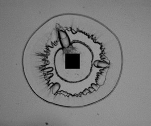
Figure 5 shows the splashing phenomenon of a 4.6 mm diameter droplet. The high-speed camera captures the images at a frame rate of 100 kfps with an exposure time of 300 ns. The black square at the centre of the water droplet is an aluminium film of size  $2.0\ \textrm {mm} \times 2.0\ \textrm {mm}$, which is larger than the focal spot of the laser to absorb all the laser energy. Figures 5(1), 6(1) and 7(1) are captured just after the lasers are triggered. In figure 5(1), the strong flash indicates that the laser focuses on the aluminium film and that the cavitation bubble has been generated. The water droplet grows with the expansion of the bubble, and a ring-shaped jet (first jet) escapes from the main droplet (see figure 5(5)). In addition, a shadow between the surfaces of the droplet and bubble is clearly observed, which indicates that the droplet surface is perturbed. Subsequently, the droplet fragments when the bubble boundary contacts the droplet surface and splashes quickly owing to the inertia of the bubble expansion. The cavitation bubble also breaks apart when contacting ambient air, and these ejections rapidly reach the escaped jet, forming a splashing phenomenon. The interested reader is referred to Appendix B for experimental and numerical investigations of the generation mechanism of the first jet shown in figure 5(5).

Figure 5. Splashing phenomenon of a water droplet with a diameter of 4.6 mm: 0–120  $\mathrm {\mu }$s expansion; 140–180 $\mathrm {\mu }$s fragmentation of the cavitation bubble. Overviews of the droplet shape (a,c), where the surface details in the red rectangle region are shown in (b,d). The resolutions of the images in (a,c) are $384\ \textrm {pixels} \times 272\ \textrm {pixels}$. See supplementary movie 1 available at https://doi.org/10.1017/jfm.2021.401.

Figure 6. Ventilating phenomenon of a water droplet with a diameter of 12 mm: 0–300  $\mathrm {\mu }$s expansion; 400–600 $\mathrm {\mu }$s contraction; and 800–1100 $\mathrm {\mu }$s collapse and rebound of a cavitation bubble. Overviews of the droplet shape (a,c,e), whose surface details in the red rectangle region are shown in (b,d,f). See supplementary movie 2.

Figure 7. Stable state of a water droplet with a diameter of 20 mm: 0–400  $\mathrm {\mu }$s expansion of the cavitation bubble; 600–800 $\mathrm {\mu }$s contraction of the cavitation bubble; 1000–1200 $\mathrm {\mu }$s second pulsation of the cavitation bubble; 1400–1800 $\mathrm {\mu }$s pulsation of broken-up bubbles. Overviews of the droplet shape (a,c), whose surface details in the red rectangle region are shown in (b,d). See supplementary movie 3.
Figure 6 shows the ventilating phenomenon of a 12 mm diameter water droplet. The settings of the high-speed camera are the same as those in figure 5. The size of the aluminium film is  $3.5\ \textrm {mm} \times 3.5\ \textrm {mm}$. In figure 6(1), a bubble cloud with an annular shape is captured around the film, which can be generated by the expansion wave after the shock wave reflects on the droplet surface (Wang et al. Reference Wang, Abe, Koita, Sun, Wang and Huang2018a). In figures 6(2) and 6(3), the water droplet grows with the expansion of the laser-induced bubble. Just before the bubble reaches its maximum size at approximately 330 $\mathrm {\mu }$s, a ring-shaped jet is also observed in this case, and Appendix B shows its generation process. As the cavitation shrinks, perturbation at the droplet surface grows remarkably and penetrates the bubble boundary, forming channels between the bubble interior and ambient air. The ambient air flows toward the interior of the bubble owing to the pressure difference, resulting in a ventilating phenomenon, as shown in figure 6(7). This indicates that interfacial instability occurs during the contraction of the bubble. At approximately 800 $\mathrm {\mu }$s, the cavitation bubble collapses, generating a pressure impulse that reverses the moving direction of the droplet surface.
Figure 7 presents a stable state for a droplet with a diameter of 20 mm. The settings of the high-speed camera are the same as those in figure 5. The size of the aluminium film is  $2.0\ \textrm {mm} \times 2.0\ \textrm {mm}$. In figure 7(1), a bubble cloud around the film is also observed just after the laser is triggered. As the cavitation bubble expands, the droplet grows to its maximum size at approximately 440 $\mathrm {\mu }$s. The ring-shaped jet is observed at the initial contraction stage, and Appendix B shows its generation mechanism. Most of the droplet surface remains smooth except for the large-amplitude distortion marked by the red circle in figure 7(4). This distortion is probably owing to the imperfect initial surface of water droplet and grows with the expansion of the bubble. In figure 7(5), some corrugations are observed at the droplet surface, and they grow until the bubble rebounds at approximately 1000 $\mathrm {\mu }$s. Interfacial instability is not induced since the perturbed surface of the droplet does not touch the bubble boundary and fragmentation is not induced. After the second collapse at approximately 1200 $\mathrm {\mu }$s, the cavitation bubble breaks up into small bubbles. As these small bubbles expand and contract, the droplet surface is slightly perturbed.
3.2. Numerical analysis of interfacial instability
Figure 8 shows comparisons of the ventilating phenomenon obtained experimentally and numerically. When similar maximum sizes and collapse times of the bubbles in the simulation match with the experimental observation, the initial bubble radius, internal pressure and internal temperature are set to 350  $\mathrm {\mu }$m, 16.5 MPa and 1500 K, respectively, referring to the numerical simulations in the study of Zeng et al. (Reference Zeng, Gonzalez-Avila, Voorde and Ohl2018). From the figure, it is found that the numerical results show good agreement with the experimental observation regarding the dynamics of the bubble and droplet. On this basis, a detailed numerical analysis of the evolution of the droplet surface is performed.

Figure 8. Dynamic behaviours of a water droplet with a diameter of 12 mm caused by the oscillation of the cavitation bubble: comparison between the experiment (left) and numerical simulation (right). The experimental results are obtained from figure 6. The simulation includes two slices at the positions of  $z=0.4$ and $z=0.75$ mm indicated by purple and black lines, respectively.
We numerically investigate the evolution of the baroclinicity and vorticity at the droplet surface. In figure 9(a-1), a surface between the bubble and droplet surfaces is induced by the expansion wave according to its propagation velocity. This indicates that the bubble clouds with annular shapes in figures 6 and 7 are induced by the tensile area behind the expansion wave. During the later stage of bubble expansion (at 300 and 400  $\mathrm {\mu }$s), baroclinicity is clearly induced and the droplet surface is perturbed, thereby forming some corrugations owing to the generated vorticity. It is because of this that the density gradient and pressure gradient are not aligned after the droplet surface is slightly perturbed. As the bubble shrinks, the surface perturbation grows rapidly. In figure 9(8) the perturbed droplet surface penetrates the bubble boundary. Upon the collapse of the bubble, a pressure impulse inversely transforms the distribution of the baroclinicity and vorticity, leading to the ejections in figure 6(10–12).

Figure 9. Surface details of a droplet with a diameter of 12 mm during expansion and contraction of the cavitation bubble obtained numerically: (a) baroclinicity and (b) vorticity. In the figure, the white and blue lines represent the slices at the positions of  $z=0.4$ and $z=0.75$ mm, respectively.
3.3. Analytical solution of the instability model
The initial conditions of the cavitation bubble play an important role in affecting the growth of the perturbation. It is difficult, however, to directly measure or observe in the experiments. In this work, the initial conditions of the bubble are estimated while matching the experimental results by the analytical model.
Figure 10(a) shows comparisons of the diameters of the cavitation bubble and the droplet obtained experimentally and analytically (the experimental results are based on figure 6). By counting the number of surface perturbations, the mode number of  $n=42$ is obtained and used in the analytical model. The diamonds and squares with error bars are the diameters of the droplet and cavitation bubble, respectively, which are averaged from 20 positions of the respective surface. Referring to the initial conditions in the simulation, we can estimate the initial condition of the bubble in this case when maximum sizes of bubbles and droplets in the analytical model match with the experimental observation. Here, initial pressure inside the bubble is $P_{in0} = 10$ MPa, the radius is $R_{b0} = 350$ $\mathrm {\mu }$m and the temperature is $T_{b0} = 1500$ K. It then follows that the pressure ratio of $P_{in0}/P_{d0} = 99.0$ and radius ratio of $R_{d0}/R_{b0} = 17.1$ for the experimental observation of figure 6. To investigate the error range of the initial conditions, we substitute the maximum and minimum of error bars into the analytical model. It is found that the maximum and minimum values of $R_{b0}$ are 366 and 336 $\mathrm {\mu }$m while that of $P_{in0}$ are 10.15 and 9.35 MPa, respectively. For the other settings in the analytical model, the thermal conductivity is $\lambda _g = 0.599$ W (m K) $^{-1}$, the heat capacity is $C_v = 4190$ J (kg K) $^{-1}$, the droplet radius is $R_{d0} = 6$ mm, the density is $\rho _{\infty } = 998$ kg m $^{-3}$, the dynamic viscosity is $\mu = 1.307\times 10^{-3}$ Pa s, the surface tension is $\sigma = 72.8 \times 10^{-3}$ N m $^{-1}$, the atmospheric pressure is $P_0 = 1.01\times 10^5$ Pa and $\eta _0 = 2 \times 10^{-7}$ m.

Figure 10. Analytical solutions of dynamic behaviours for a water droplet with a diameter of 12 mm obtained by the instability model at  $n = 42$. In (a), the symbols with error bars are obtained based on experimental observation in figure 6. The green and red curves are analytical solutions of the diameters of cavitation bubbles and water droplets, respectively. In (b), the blue and orange curves are analytical solutions for the acceleration and perturbation of the droplet surface, respectively. (a) Time variations with diameters of cavitation bubble and water droplet and (b) time variations with acceleration of droplet surface and dimensionless perturbation.
As shown in figure 10(a), the bubble shrinks faster in the experiment than that in the analytical model during the contraction of the cavitation bubble. This is because the first jet takes away part of the mass and momentum of the droplet. With the exception of the errors induced by the loss of the mass and momentum, the analytical model describes the dynamics of the cavitation bubble and the droplet well. According to the direction of the surface acceleration, an unstable period of the droplet surface is qualitatively predicted as indicated by red area in figure 10(b). Here, the direction of the bubble expansion is set as positive. It is found that the surface perturbations appear to grow exponentially at the later stage of expansion and the initial stage of contraction of the bubble. Eventually, the amplitude of the dimensionless perturbations reach the first peak,  $\eta ^{\prime }_{max}=\eta _{max}/R_{d0}$, 0.18-fold droplet radius at the collapse of the bubble.
Next, the analytical model is solved to investigate how the mode number  $n$ and initial perturbations $\eta _0$ affect the evolution of the surface perturbation. By using the Wentzel–Kramers–Brillouin approximation, we can obtain a function of the perturbation $\eta$, namely, $\eta (t)\sim \eta _0 \exp (S_n(t))$. Here, $S_n$ is the growth rate of the perturbation and can be expressed as
 \begin{equation} S_n={\pm}\sqrt{ak_wA}, \end{equation}
where  $a$ is the acceleration, $A$ is the Atwood number and $k_w = n/R_{d0}$ is the wavenumber. We can obtain a relation between the peak of dimensionless perturbation $\eta ^{\prime }_{max}$ and mode number $n$, namely,
 \begin{equation} \eta^{\prime}_{max}\sim\frac{\eta_{0}^{}}{R_{d0}}\textrm{e}^{{\pm}\sqrt{n}}. \end{equation}
 Figure 11(a) shows the estimation of the peak of dimensionless perturbation for a 12 mm diameter droplet under different mode numbers. The other initial conditions are the same as those in figure 10. The abscissa is the mode number  $n$ and the ordinate is the peak of the dimensionless perturbation $\eta ^{\prime }_{max}$. The peak of the perturbation increases as an exponential function of $\sqrt {n}$. It is relatively easy for a large mode number to result in interfacial instability of the droplet. A coefficient of 10.82 is obtained by fitting the curve using (3.2), as shown in figure 11(a). Here, the dimensionless initial perturbation is $\eta _{0}^{\prime } = \eta _0/ R_{d0} = 3.33\times 10^{-5}$. As a result, (3.2) can be effectively used to estimate the peak amplitude of the perturbation under different mode numbers.

Figure 11. Estimation of the peak of the dimensionless perturbation for a water droplet with a diameter of 12 mm at  $P_{in0}/P_{d0}=99.0$ and $R_{d0}/R_{b0}=17.1$ for different (a) mode numbers and (b) initial perturbations. In (a), the blue line represents the analytical solution of the model and the orange line is the fitting line of (3.2). In (b), the solid lines represent the analytical solutions of the model and the dashed lines are the estimates of (3.2).
In addition, the estimations of the dimensionless perturbation peak are shown in figure 11(b) under different initial perturbations. The solid lines are the analytical solutions of the instability model when the dimensionless initial perturbation is 0.5, 2, 4, 10 and 20 times,  $\eta _0^{\prime } = 3.33 \times 10^{-5}$. The dashed lines are the estimations obtained with (3.2) when using the coefficient of 10.82. The estimated lines agree well with the analytical solutions. This suggests that the peak of the dimensionless perturbation is proportional to the initial perturbation and that (3.2) accurately describes how the mode number $n$ and initial perturbation $\eta _0$ affect the perturbation growth.
3.4. Phase diagram of interfacial instability
The analytical model is solved with different initial conditions of the bubbles and droplets. Two dimensionless parameters of the surface perturbation are defined to determine the instability and stability regimes of the droplet surface. One parameter is  $\hat {\eta }_{ins}$
 \begin{equation} \hat{\eta}_{ins}=\frac{\dot{R_b}}{\rvert \dot{R_b}\rvert}\frac{\eta_{max}}{{\rm \Delta} R}= \frac{\dot{R_b}}{\rvert \dot{R_b}\rvert}\frac{\eta_{max}}{R_d-R_b}, \end{equation}
where  $\eta _{max}$ is the maximum perturbation of the droplet surface and $R_d$ and $R_b$ are the radii of the droplet and bubble at this moment, respectively. The positive and negative signs of the term $\dot {R_b}/\rvert \dot {R_b}\rvert$ represent the expansion and contraction of the bubble, respectively. This means that interfacial instability occurs when the surface perturbation touches the bubble boundary, i.e. the amplitude of the perturbation is equal to the difference between the bubble radius and droplet radius. Consequently, splashing and ventilating phenomena occur for $\hat {\eta }_{ins}\geq 1$ and $\hat {\eta }_{ins} \leq -1$, respectively.
The other dimensionless parameter is  $\hat {\eta }_{sta}$, which is used to determine the stability regime where the bubble boundary is not penetrated despite small-amplitude perturbations. Referring to the study of Zeng et al. (Reference Zeng, Gonzalez-Avila, Voorde and Ohl2018), $\hat {\eta }_{sta}=|\eta _{max}/R_{d0}| = 0.1$ is applied as a threshold. Consequently, we obtain the phase diagram shown in figure 12(a). The mode number $n$ is 42. The dimensionless pressure $P_{in0}/P_{d0}$ and radius $R_{d0}/R_{b0}$ are used as the ordinate and abscissa, respectively. In the phase diagram, the regimes of splashing, ventilating and a stable state are presented using red, blue and green, respectively. There is a transition zone between the ventilating phenomenon and stable state, which is bounded by the lines of $\hat {\eta }_{ins} = -1$ and $\hat {\eta }_{sta} = 0.1$.

Figure 12. Phase diagram of the interfacial instability of 2-D water droplets at  $n=42$: phase diagram (a) and typical cases (b). In (a), the symbols denote three regimes: splashing ( $\blacklozenge$); ventilating ( $\bullet$); and the stable state ( $\blacktriangle$). The white and black symbols denote the results obtained experimentally and numerically, respectively. In (b), E-1 (figure 5), E-2, E-3 (figure 6) and E-4 (figure 7) are obtained experimentally. S-1, S-2, S-3 and S-4 are obtained numerically. The droplet radius $R_d$ is presented by arc lines, along with the perturbation $\eta$.
Figure 12(b) shows typical examples in the respective regime. The variables E and S represent the results obtained from experiments and simulations, respectively. The splashing phenomenon occurs during bubble expansion in the high-energy and small-droplet regime. We obtain  $|\eta _{max}/R_{d0}| = 0.45$ for E-1 and $|\eta _{max}/R_{d0}| = 0.55$ for S-1. For E-2 and S-2, the perturbations penetrate the bubble boundary during the initial contraction of the bubble, the values of $|\eta _{max}/R_{d0}|$ are 0.22 and 0.14, respectively. For E-3 and S-3, the perturbations grow until the cavitation bubble collapses, the values of $|\eta _{max}/R_{d0}|$ are 0.30 and 0.35, respectively. E-4 and S-4 are cases in the regime of the stable state, where the interfacial instability is not induced despite some corrugations at the droplet surface. The other results obtained experimentally and numerically are plotted in the phase diagram in the same way (see figure 12a). Here, the initial conditions of the cavitation bubble in the experiments are obtained by solving the analytical model, as shown in figure 10. We obtain $P_{in0}/P_{d0} = 99.0$ and $R_{d0}/R_{b0} = 5.7$ for figure 5, $P_{in0}/P_{d0} = 99.0$ and $R_{d0}/R_{b0} = 17.1$ for figure 6 and $P_{in0}/P_{d0} = 99.0$ and $R_{d0}/R_{b0} = 28.6$ for figure 7.
The phase diagram for a 2-D cylindrical droplet shows some similarities and differences compared with that of a spherical droplet (Gonzalez Avila & Ohl Reference Gonzalez Avila and Ohl2016). The splashing and stable state of the droplet are also observed for a spherical geometry. However, the ventilating phenomenon is observed in the experiment for the first time. The perturbed droplet surface in this case can touch or even penetrate the bubble boundary, forming channels between the bubble interior and ambient air. As Zeng et al. (Reference Zeng, Gonzalez-Avila, Voorde and Ohl2018) suggested, the corrugated surface of spherical droplet does not allow a closer look at the cavitation bubble in the experiment. Consequently, it is difficult to observe clearly the ventilating phenomenon in a spherical droplet. In the present study the channels are observed clearly and the perturbations at the surface are measured precisely so that the interfacial instability is accurately determined. From the perspective of energy transfer, interfacial instability occurs when the droplet obtains enough energy from the oscillation of the bubble. Thus, the relationship between the pressure and radius ratios is obtained as
 \begin{equation} \frac{P_{in0}}{P_0}\sim C_n\left(\frac{R_{d0}}{R_{b0}}\right)^2, \end{equation}
where  $C_n$ is the bubble-to-droplet energy conversion factor and depends mainly on the mode number. Considering the effect of the mode number in figure 11, $C_n$ can be expressed as
 \begin{equation} C_n=C_2\ \textrm{e}^{{\pm} \sqrt{n}}+C_3. \end{equation}
 Figure 13 shows boundary curve lines between the stability and instability regimes of the droplet surface at  $n=20$, 25, 30, 40, 45 and 50. The area of the stability regime decreases as the mode number increases. This is because the wavenumber increases with the mode number, thereby increasing the growth rate of the perturbation according to (3.1). Consequently, the perturbations grow faster for a larger mode number. Overall, the estimates show good agreement with the analytical solutions. Therefore, (3.4) can be used to predict the stability and instability regimes for a water droplet.

Figure 13. Boundary lines between the stability and instability regimes for 2-D water droplets caused by internal volume oscillation at  $n=20$, 25, 30, 40, 45 and 50. The solid lines represent the analytical solutions of the instability model. The dashed lines are the estimates of (3.4) when using $C_2=11.17$ and $C_3=0.372$. The left and right regimes of each curve represent instability and stability, respectively.
4. Conclusion
In this paper, we investigate the interfacial instability of a water droplet induced by internal volume oscillation using a combination of experiments, numerical simulations and analytical modelling. In the experiments droplets of various sizes are generated by injecting water into a narrow gap, and a pulsed laser is focused on the interior of the droplet to generate a cavitation bubble. Three distinct characteristics of droplet deformation are observed, namely, (i) splashing, (ii) ventilating and (iii) a stable state.
The ventilating phenomenon is experimentally observed for the first time. As the bubble shrinks, the perturbed droplet surface moves toward its centre and penetrates the bubble boundary so that the bubble interior is connected to ambient air, resulting in the ventilation phenomenon. The phenomena of splashing and a stable state, which were reported for a spherical droplet, were also found in the present study.
To analyse the growth of perturbations at the droplet surface, an analytical model comprising (i) a linear model to describe the evolution of the interfacial instability and (ii) a bubble oscillation model is developed. A phase diagram distinguishing various phenomena of the droplet is obtained by solving the analytical model and is verified by the experimental and numerical results.
Two dimensionless parameters of surface perturbation,  $\hat {\eta }_{ins}$ and $\hat {\eta }_{sta}$, are defined to distinguish the different regimes of the phase diagram. Interfacial instability occurs when the perturbed surface penetrates the bubble boundary, i.e. $\rvert \hat {\eta }_{ins} \rvert \geq 1$. Splashing and ventilating phenomena occur for $\hat {\eta }_{ins}\geq 1$ and $\hat {\eta }_{ins}\leq -1$, respectively. The droplet is considered to be stable as fragmentation does not occur despite small-amplitude perturbations, and the regime of the stable state is $\hat {\eta }_{sta}\leq 0.1$, which is the other dimensionless parameter. There is a transition zone between the regimes of ventilating and stable states, which is bounded by $\hat {\eta }_{ins} = -1$ and $\hat {\eta }_{sta} = 0.1$.
The experimental observations and numerical results show that the location of the first jet escaping from the droplet depends on the initial shape of the water surface from the side view as mentioned in Appendix B. Therefore, it is of great interest to investigate the evolution of the first jet under different initial shapes of the water surface by changing the contact angles of the plates.
Supplementary movies
Supplementary movies are available at https://doi.org/10.1017/jfm.2021.401.
Funding
The authors would like to thank the National Natural Science Foundation of China (11802311, 11772340 and 11672315), the Youth Innovation Promotion Association CAS (Y201906) and the Foundation of National Key Laboratory of Shock Wave and Detonation Physics (JCKYS2018212007).
Declaration of interests
The authors report no conflict of interest.
Appendix A. Grid independence
We analyse the grid independence by developing three types of grids, namely, coarse, medium and fine. Table 2 shows the numbers of cells and simulation times for each grid. Here, the simulation time is the time taken to calculate the first pulsation of the cavitation bubble. For each grid, the resolution near the walls of the narrow gap was high enough to analyse the boundary layer.
Figure 14 shows the temporal evolutions of the bubble radius and the position of the outer edge of the droplet during the first pulsation under different grids. The detailed information is given in table 3. Note that the initial conditions are the same as those in figure 8, namely, the radius is  $R_{b0} = 350\ {\mathrm {\mu }}$m, the temperature is $T_0 = 1500$ K and the pressure is $P_{in0} = 16.5$ MPa. As shown in figure 14, all the results obtained with various grids are consistent regarding the evolution of the bubble radius. As to the outer edge of the droplet, the results of the medium grid are consistent with those of the fine grid, whereas there are some differences in the later stage of the first pulsation for the coarse grid. Consequently, considering computational cost and efficiency, we used the medium grid in all simulations.

Figure 14. Temporal evolutions of the bubble radius and outer edge of the droplet during the first pulsation of the cavitation bubble using different grids.
Table 3. Details of the bubble radius and outer edge of the droplet for coarse, medium and fine grids.

Appendix B. Generation of the ring-shaped jet
To investigate the generation mechanism of the ring-shaped jet, we observed the side view of the narrow gap. The high-speed camera captures the images at a frame rate of 100 kfps with an exposure time of 300 ns. The resolution of the images is  $1280\ \textrm {pixels} \times 192\ \textrm {pixels}$. In figure 15(1), the surface of the droplet in the narrow gap remains curved because of surface tension. As the bubble expands, the curved surface grows gradually, forms a water dome at 200 $\mathrm {\mu }$s and transforms into a jet, as shown in figure 15(5). Compared with the top view in figure 5, we can conclude that the jet created at the middle of the droplet surface is the ring-shaped first jet. The position of the jet is slightly above the centre of the gap, which may be owing to the three-dimensional effect of initial expansion of the cavitation bubble. As the bubble rebounds, two further jets form at both sides of the first jet and are called the second jet. Then, the third pulsation results in the generation of the third jets between the first and second jets.

Figure 15. Side view of behaviours of a water droplet in a narrow gap with a diameter of 8 mm: 0–200  $\mathrm {\mu }$s expansion; 300–500 $\mathrm {\mu }$s contraction; 600–900 $\mathrm {\mu }$s second pulsation; and 1000 $\mathrm {\mu }$s third pulsation of cavitation bubble. See supplementary movie 4.
The first jet is similar to a highly focused supersonic microjet in other studies (Tagawa et al. Reference Tagawa, Oudalov, Visser, Peters, Meer, Sun, Prosperetti and Lohse2012; Peters et al. Reference Peters, Tagawa, Oudalov, Sun, Prosperetti, Lohse and Meer2013). Tagawa et al. (Reference Tagawa, Oudalov, Visser, Peters, Meer, Sun, Prosperetti and Lohse2012) argued that the supersonic microjet is induced by ‘kinematic focusing’ of the liquid. This is because the impulsive acceleration or pressure converges toward the centre of curvature of the droplet surface. A shock wave is the dominant factor in the kinematic focusing of the liquid when it is reflected at the surface in their study. However, in the present study, when the generated shock wave reaches the droplet surface, the pressure behind it is of the order of dozens of MPa, even several MPa according to the study of Wang et al. (Reference Wang, Abe, Nishio, Wang and Huang2018b). Furthermore, the droplet surface can achieve great acceleration owing to the initial expansion of cavitation bubble, as shown in figure 10(b). Consequently, the bubble expansion may be one of the most important factors in generating the first jet in the present study.
Figure 16(a) shows the velocity field of a droplet with a diameter of 12 mm during the first pulsation of the cavitation bubble obtained with numerical simulation. As shown in figure 16(a-2), we observe the focusing of the flow at the droplet as marked by the red ellipse, which can be induced by the shock wave according to its propagation velocity. This indicates that the initial perturbation is stimulated by the shock wave. As the bubble expands, the droplet surface grows gradually, forming the first jet. Given the velocity curve of the jet in figure 16(b), the droplet surface is accelerated during two periods. From the perspective of the time scale, it is found that Period 1 is mainly caused by the propagation of shock wave, while Period 2 is dominated by the expansion of the bubble. Subsequently, Period 3 shows that the droplet surface decelerates owing to the surface tension until a small droplet is generated at the tip of the first jet at approximately 600  $\mathrm {\mu }$s. As a result, the generation and acceleration of the jet is caused by the combination of the shock wave and expansion of the cavitation bubble.

Figure 16. Evolution of the ring-shaped jet for a droplet with a diameter of 12 mm obtained numerically: (a) velocity field; (b) velocity at the surface centre. In (a), the cross section is at  $z=0.4$ mm, and the focusing of the flow at the droplet surface is induced by the propagation of the shock wave, as indicated by the red ellipse. In (b), the velocity at the centre of the droplet surface is that of the ring-shaped jet.


 Open access