


1. Introduction
A porous medium refers to a material consisting of a solid matrix with interconnected voids. Flows in porous media are often laminar due to the low Reynolds number. However, at certain conditions, the Reynolds number based on the pore scale might exceed its critical value for laminar–turbulence transition and thus the flow becomes turbulent.
Turbulence in porous media can be often found in canopy flows. The examples include the flows in porous canopies made of trees, vegetation or buildings (Meroney Reference Meroney2007). These canopies usually have large porosities (typically >90%, see Ghisalberti & Nepf (Reference Ghisalberti and Nepf2009)) and high permeability ( ${10^{ - 4}}\text{--}{10^{ - 1}}\;{\textrm{m}^2}$, see Rubol, Ling & Battiato (Reference Rubol, Ling and Battiato2018)). Whether macroscopic turbulence can survive or not in porous media is a significant question for these applications. It might enhance pollutant removal in wetland (Serra, Fernando & Rodriguez Reference Serra, Fernando and Rodriguez2004), benefit vegetation by augmenting nutrient uptake and/or gas exchange (Nepf Reference Nepf2012), influence biological and ecological mechanisms (de Langre Reference de Langre2008) and help to blow air pollutants in a city away efficiently. One type of macroscopic turbulence is generated due to Kelvin–Helmholtz stability which occurs at the canopy interface. Many studies about this type of macroscopic turbulence can be found, see Breugem, Boersma & Uittenbogaard (Reference Breugem, Boersma and Uittenbogaard2006), Suga (Reference Suga2016), Kim et al. (Reference Kim, Blois, Best and Christensen2020) as examples. Nepf (Reference Nepf2012) indicated that the lower canopy, which is far below the interface, is associated with pore-scale turbulence. However, when the lower canopy has more than one length scale, the large-scale turbulence stimulated by the large porous elements (e.g. tree trunks in a forest canopy) can be also treated as macroscopic turbulence. This macroscopic turbulence might survive if it cannot be suppressed by the small porous elements (e.g. tree leaves, stems or grasses).
Possibility for survival of macroscopic turbulence in porous media has been intensively studied in past years. There are two distinct views on this question. According to the first view, macroscopic turbulence in porous media is believed to be possible, see Lee & Howell (Reference Lee and Howell1991) and Antohe & Lage (Reference Antohe and Lage1997). Transport of turbulence kinetic energy should be accounted for when there is macroscopic turbulence. The examples include the models by Prescott & Incropera (Reference Prescott and Incropera1995), Antohe & Lage (Reference Antohe and Lage1997), Getachew, Minkowycy & Lage (Reference Getachew, Minkowycy and Lage2000) and de Lemos (Reference de Lemos2012). Macroscopic turbulence models have also been used to simulate flow in a porous matrix represented by a periodic array of square cylinders (Kazerooni & Hannani Reference Kazerooni and Hannani2009; Kundu, Kumar & Mishra Reference Kundu, Kumar and Mishra2014). Belcher, Harman & Finnigan (Reference Belcher, Harman and Finnigan2012) suggested that canopy flows are characterized by the drag length scale rather than the depth of the canopy. However, it is not clear if the drag length scale is related to macroscopic turbulence.
In the second view, macroscopic turbulence is impossible because of the limitation on the size of turbulent eddies imposed by the pore scale, see Nield (Reference Nield1991, Reference Nield2001), Nakayama & Kuwahara (Reference Nakayama and Kuwahara1999) and Kuwahara et al. (Reference Kuwahara, Kameyama, Yamashita and Nakayama1998) as examples. Using an experimental method, Tanino & Nepf (Reference Tanino and Nepf2008) suggested that the integral length scale of turbulence is determined by the minimum value of the surface-to-surface distance between cylinders and the cylinder diameter, both of which belong to pore scales. They further proposed that only turbulent eddies with mixing length scales greater than the cylinder diameter contribute significantly to dispersion, which is the transport of solute due to both time fluctuations and spatial deviations of microscopic velocity and species concentration. Through a direct numerical simulation (DNS) study of turbulent flows in a porous medium made of square cylinders, Jin et al. (Reference Jin, Uth, Kuznetsov and Herwig2015) concluded the turbulent eddies are generally restricted by the pore size, leading to the pore-scale prevalence hypothesis (PSPH). Uth et al. (Reference Uth, Jin, Kuznetsov and Herwig2016) and Jin & Kuznetsov (Reference Jin and Kuznetsov2017) confirmed the PSPH with the DNS results for different geometries of the porous matrix. Rao, Kuznetsov & Jin (Reference Rao, Kuznetsov and Jin2020) developed a macroscopic model based on the PSPH, in which microscopic turbulence is modelled.
However, the PSPH has a boundary of validity. If the porosity approaches unity, the effect of the porous matrix on the flow will disappear. Macroscopic turbulence will survive under such a condition. In Uth et al. (Reference Uth, Jin, Kuznetsov and Herwig2016), a second (large) element is imposed in the porous matrix; it can stimulate strong large-scale turbulence. The DNS results show that, when the porosity for the porous matrix made of small length scales is large enough, the macroscopic turbulence seems to survive. Chu, Weigand & Vaikuntanathan (Reference Chu, Weigand and Vaikuntanathan2018) and Srikanth et al. (Reference Srikanth, Huang, Su and Kuznetsov2018) also confirmed the existence of large turbulent structures for flows with large porosities. Therefore, the PSPH should have a boundary of validity, out of which macroscopic turbulence might survive.
The purpose of this study is to find out in what conditions the large turbulent structures might survive. To achieve this goal, the turbulent flows in a porous matrix with two length scales will be calculated by using both DNS and macroscopic simulation methods. Strong large-scale turbulence can be stimulated by the large porous matrix. The spacing between small porous elements is varied to obtain different porosity values. The PSPH macroscopic model proposed by Rao et al. (Reference Rao, Kuznetsov and Jin2020) will be used in the macroscopic simulation. While the microscopic turbulence is modelled in the PSPH model, it is possible to resolve the macroscopic turbulence directly when it can survive. The DNS and macroscopic simulation results will verify and complement each other in the study.
2. Geometry of the porous matrix
The porous matrix in this study is made of two-dimensional staggered arrays of bars with the element size  ${d_l}$ and spacing ${s_l}$ and three-dimensional aligned arrays of spheres or cubes with the element size ${d_s}$ and spacing ${s_s}$, see figure 1(a,b). The computational domain is a representative elementary volume (REV) for the large porous element. The ratio between the large pore size ${s_l}$ and the bar size ${d_l}$ has a fixed value $({s_l}/{d_l} = 2)$. The same domain size $(2{s_l} \times 2{s_l} \times {s_l})$ is used for all test cases.

Figure 1. Porous matrices used in the study. (a) A porous matrix with two length scales (made of cubes and spheres); (b) a REV for the small porous element; (c) a porous matrix with only small pore scale (made of spheres); (d) a porous matrix with only large pore scale (made of bars).
The porous matrices are made of the same large porous elements (staggered bars) but different numbers of REVs have been studied in Jin et al. (Reference Jin, Uth, Kuznetsov and Herwig2015). The numerical results show that the computational domain in this study is large enough to calculate the length scale of turbulence at the centre of a REV accurately.
The flow is in  ${x_1}$ direction. The Reynolds numbers for the large and small elements are defined as
 \begin{equation}R{e_s} = \frac{{{u_m}{d_s}}}{\nu },\quad R{e_l} = \frac{{{u_m}{d_l}}}{\nu },\end{equation}
where  ${u_m}$ is the mean seepage velocity.
The Reynolds number  $R{e_K}$ for a generic porous matrix (GPM) made of small porous elements can be defined as
 \begin{equation}R{e_K} = \frac{{{u_m}\sqrt K }}{\nu },\end{equation}
where K is the permeability. The Darcy number  $Da$ for the GPM is defined as
 \begin{equation}Da = K/d_l^2,\end{equation} ${\phi _s}$ denotes the porosity for the porous matrix made of small porous elements. For the porous matrix made of spheres, ${\phi _s}$ is calculated as
 \begin{equation}{\phi _s} = 1 - \frac{{\rm \pi} }{6}{\left( {\frac{{{d_s}}}{{{s_s}}}} \right)^3}.\end{equation}
For the porous matrix made of cubes,  ${\phi _s}$ is calculated as
 \begin{equation}{\phi _s} = 1 - {\left( {\frac{{{d_s}}}{{{s_s}}}} \right)^3}.\end{equation}
In order to make the comparison, we have also calculated the flows in porous matrices with only one length scale. They are made of either only large porous elements (figure 1c) or only small porous elements (figure 1d).
3. Governing equations and numerical methods
3.1. DNS
In DNS, the transient Navier–Stokes equations accounting for all scales of turbulent motions are solved directly without using any turbulence model. For flows in porous media, the detailed pore-scale geometry is also resolved. The governing equations for an incompressible flow read
 \begin{gather}\frac{{\partial {u_i}}}{{\partial {x_i}}} = 0,\end{gather}
 \begin{gather}\frac{{\partial {u_i}}}{{\partial t}} + \frac{{\partial {u_i}{u_j}}}{{\partial {x_j}}} ={-} \frac{{\partial p}}{{\partial {x_i}}} + \nu \frac{{{\partial ^2}{u_i}}}{{\partial x_j^2}} + {g_i},\end{gather}
where  ${g_i}$ is the applied pressure gradient in the momentum equation which maintains a constant flow rate. A set of general units (L for length and T for time) are used in the study so that the numerical results can be applied in any system of units.
The governing equations (3.1)–(3.2) are solved by using a lattice-Boltzmann method (LBM). The basic equation for the present LBM is a discretized version of the Boltzmann equation (Aidun & Clausen Reference Aidun and Clausen2009). The collision operator is modelled by the Bhatnagar–-Gross–Krook (BGK) model (Bhatnagar, Gross & Krook Reference Bhatnagar, Gross and Krook1954),
 \begin{equation}{f_i}(\boldsymbol{x} + {\boldsymbol{\xi }_{\boldsymbol{i}}}\mathrm{\Delta }t,t + \mathrm{\Delta }t) - {f_i}(\boldsymbol{x},t) ={-} \frac{1}{\tau }(\,f_{i}(\boldsymbol{x},t) - f_i^{eq}(\boldsymbol{x},t)),\end{equation}
where  ${\boldsymbol{\xi }_{\boldsymbol{i}}}$ is a discrete particle velocity, ${f_i}(\boldsymbol{x},t)$ is the number distribution of molecules at a position $\boldsymbol{x}$ at a time t along with direction i, $f_i^{eq}(\boldsymbol{x},t)$ is the equilibrium form of ${f_i}(\boldsymbol{x},t)$ and $\tau $ is the relaxation time which determines the kinematic viscosity (see Chen & Doolen Reference Chen and Doolen1998).
With the help of the Chapman–Enskog expansion (see Chen & Doolen Reference Chen and Doolen1998), (3.3) solves the incompressible Navier–Stokes equations (3.1)–(3.2) by streaming and collision processes. The left-hand side term represents the streaming process while the right-hand side term represents the collision process. Equation (3.3) is a linear partial differential equation and the meshes are uniformly distributed in all directions, which leads the LBM to run efficiently on massively parallel architectures. The bounce-back model with numerical approximation of second order is applied to the wall surfaces of the porous elements. More details can be found in Mohamad (Reference Mohamad2011).
3.2. Macroscopic simulation
Direct numerical simulation is the most accurate method for studying turbulent flows in porous media, however, it is extremely expensive, particular for porous media with high porosities and low Darcy numbers. So, some cases are calculated by using macroscopic simulation. Some DNS cases are calculated again using the macroscopic simulation solver for validation.
The large porous elements (bars) are still fully resolved in macroscopic simulation while the small porous elements are modelled. Volume averaging (3.1)–(3.2) in each REV and using the theorem of local volumetric average (Slattery Reference Slattery1967; Whitaker Reference Whitaker1969, Reference Whitaker1999; Gray & Lee Reference Gray and Lee1977), the macroscopic equations for flows in a porous medium can be obtained, expressed as
 \begin{gather}\frac{{\partial {u_{Di}}}}{{\partial {x_i}}} = 0,\end{gather}
 \begin{gather}\frac{{\partial {u_{Di}}}}{{\partial t}} + \frac{{\partial ({u_{Di}}{u_{Di}}/\phi )}}{{\partial {x_j}}} ={-} \frac{{\partial (\phi {{\langle p\rangle }^i})}}{{\partial {x_i}}} + \phi {g_i} - \phi {R_i} + \nu \frac{{{\partial ^2}{u_{Di}}}}{{\partial x_j^2}} - \frac{{\partial (\phi {{\langle {}^i{u_i}{}^i{u_j}\rangle }^i})}}{{\partial {x_j}}}.\end{gather}
 The operator  ${\langle \cdot \rangle ^i}$ denotes volume averaging over the fluid region of an REV. Here ${u_{Di}} = \phi {\langle {u_i}\rangle ^i}$ is the superficial velocity and ${R_i}$ denotes the total drag caused by the effect of the porous matrix. The spatial deviation ${}^i{u_i}$ is the difference between the value at a point and its intrinsic average, calculated as ${}^i{u_i} = {u_i} - {\langle {u_i}\rangle ^i}$.
Rao et al. (Reference Rao, Kuznetsov and Jin2020) assumed in the PSPH model that macroscopic turbulence does not exist when the porosity is not very large, so only microscopic turbulence is accounted for in this model. However, it is still possible to capture the macroscopic turbulence directly using this model if it survives. Now  ${R_i}$ is decomposed into a drag term $R_i^\ast $ which is determined by ${u_{Di}}$ and the residual drag term ${R_i} - R_i^\ast $ related to the gradient of ${u_{Di}}$. Making a Taylor extension for $R_i^\ast $ with respect to a local Reynolds number $R{e_K} = \sqrt K |{{\boldsymbol{u}_D}} |/\nu $ and taking the first two leading-order terms, we have
 \begin{equation}R_i^\ast = \frac{\nu }{K}{u_{Di}}(1 + {c_{F1}}R{e_K}).\end{equation}
Equation (3.6) is identical to the Forchheimer extension of the Darcy term (Lage & Antohe Reference Lage and Antohe2000). For the small porous elements under consideration (aligned spheres or cubes), the Forchheimer coefficient  ${c_{F1}}$ is set to 0.1, see Nield & Bejan (Reference Nield and Bejan2017) and Rao et al. (Reference Rao, Kuznetsov and Jin2020).
The sum of the momentum dispersion  $\phi {\langle {}^i{u_i}{}^i{u_j}\rangle ^i}$, molecular diffusion $2\nu {s_{Dij}}$ and drag due to the velocity gradient ${R_i} - R_i^\ast $ is modelled using a Laplacian term ${L_i}$, expressed as
 \begin{equation}{L_i} = \phi ({R_i} - R_i^\ast ) + \nu \frac{{{\partial ^2}{u_{Di}}}}{{\partial x_j^2}} - \frac{{\partial (\phi {{\langle {}^i{u_i}{}^i{u_j}\rangle }^i})}}{{\partial {x_j}}} = \frac{\partial }{{\partial x_j}}(2\tilde{\nu }{s_{Dij}})\; ,\end{equation}
where  $\tilde{\nu }$ is an effective viscosity. Rao et al. (Reference Rao, Kuznetsov and Jin2020) introduced another local Reynolds number to model the effective viscosity $\tilde{\nu }$, defined as
 \begin{equation}R{e_d} = \frac{{K|{{\boldsymbol{s}_D}} |}}{\nu },\end{equation}
where  ${\boldsymbol{s}_D}$ is the strain rate tensor of the superficial velocity ${\boldsymbol{u}_D}$. Making a Taylor expansion with respect to $R{e_d}$ for $\tilde{\nu }/\nu $ and taking the first two leading-order terms, we have
 \begin{equation}\tilde{\nu }/\nu = {c_{B1}} + {c_{B2}}R{e_d}.\end{equation}
The model coefficients K,  ${c_{F1}}$, ${c_{B1}}$ and ${c_{B2}}$ are all geometric parameters which are independent of the flow condition. They are determined empirically in this study. The permeability K can be approximated by the Carman–Kozeny equation (Kozeny Reference Kozeny1927; Carman Reference Carman1956), expressed as
 \begin{equation}K = \frac{{D_{P2}^2{\phi ^3}}}{{{c_K}{{(1 - \phi )}^2}\textrm{\; \; }}},\end{equation}
where  $D_{P2}$ is an effective average particle or fibre diameter. The model coefficient ${c_K}$ has the value 180, and ${c_{B1}}$ and ${c_{B2}}$ are calculated using the correlations in Rao et al. (Reference Rao, Kuznetsov and Jin2020), they are
 \begin{gather}{c_{B1}} = 49.63\textrm{\; } \times \frac{{{{(1 - \phi )}^2}}}{{{\phi ^{0.5}}}} + 1,\end{gather}
 \begin{gather}{c_{B2}} = 0.79 \times \frac{{{{(1 - \phi )}^2}}}{{{\phi ^3}}}.\end{gather}
Substituting (3.6) and (3.7) into (3.5), normalizing with the mean velocity  ${u_m}$ and the large element size ${d_l}$, the following dimensionless macroscopic equations can be obtained:
 \begin{gather}\frac{{\partial {{\mathord{\buildrel{\lower3pt\hbox{$\scriptscriptstyle\smile$}} \over u} }_{Di}}}}{{\partial {{\mathord{\buildrel{\lower3pt\hbox{$\scriptscriptstyle\smile$}} \over x} }_i}}} = 0,\end{gather}
 \begin{gather}\frac{{\partial {{\mathord{\buildrel{\lower3pt\hbox{$\scriptscriptstyle\smile$}} \over u} }_{Di}}}}{{\partial \mathord{\buildrel{\lower3pt\hbox{$\scriptscriptstyle\smile$}} \over t} }} + \frac{{\partial ({{\mathord{\buildrel{\lower3pt\hbox{$\scriptscriptstyle\smile$}} \over u} }_{Di}}{{\mathord{\buildrel{\lower3pt\hbox{$\scriptscriptstyle\smile$}} \over u} }_{Di}}/\phi )}}{{\partial {{\mathord{\buildrel{\lower3pt\hbox{$\scriptscriptstyle\smile$}} \over x} }_j}}} ={-} \frac{{\partial (\phi {{\langle \mathord{\buildrel{\lower3pt\hbox{$\scriptscriptstyle\smile$}} \over p} \rangle }^i})}}{{\partial {{\mathord{\buildrel{\lower3pt\hbox{$\scriptscriptstyle\smile$}} \over x} }_i}}} + \phi {\mathord{\buildrel{\lower3pt\hbox{$\scriptscriptstyle\smile$}} \over g} _i} - {\mathord{\buildrel{\lower3pt\hbox{$\scriptscriptstyle\smile$}} \over R} _i} + {\mathord{\buildrel{\lower3pt\hbox{$\scriptscriptstyle\smile$}} \over L} _i},\end{gather}
where  $\smallsmile$ denotes a dimensionless variable. The dimensionless drag and Laplacian terms are calculated as
 \begin{gather}{\mathord{\buildrel{\lower3pt\hbox{$\scriptscriptstyle\smile$}} \over R} _i} = \frac{\phi }{{DaR{e_l}}}{\mathord{\buildrel{\lower3pt\hbox{$\scriptscriptstyle\smile$}} \over u} _{Di}} + \frac{{\phi {c_{F1}}}}{{Da^{1/2}}}\left|{{{\boldsymbol{\mathord{\buildrel{\lower3pt\hbox{$\scriptscriptstyle\smile$}} \over u} }}_D}} \right|{\mathord{\buildrel{\lower3pt\hbox{$\scriptscriptstyle\smile$}} \over u} _{Di}},\end{gather}
 \begin{gather}{\mathord{\buildrel{\lower3pt\hbox{$\scriptscriptstyle\smile$}} \over L} _i} = 2\frac{\partial }{{\partial x_j}}\left[ {\left( {\frac{{{c_{B1}}}}{{R{e_l}}} + {c_{B2}}Da\left|{{{\boldsymbol{\mathord{\buildrel{\lower3pt\hbox{$\scriptscriptstyle\smile$}} \over s} }}_D}} \right|} \right){{\hat{s}}_{Dij}}} \right].\end{gather}
 When  $R{e_l}$ is high enough $(R{e_l} \to \infty )$, (3.15) and (3.16) can be simplified as
 \begin{gather}{\mathord{\buildrel{\lower3pt\hbox{$\scriptscriptstyle\smile$}} \over R} _i} = \frac{{\phi {c_{F1}}}}{{Da^{1/2}}}\left|{{{\boldsymbol{\mathord{\buildrel{\lower3pt\hbox{$\scriptscriptstyle\smile$}} \over u} }}_D}} \right|{\mathord{\buildrel{\lower3pt\hbox{$\scriptscriptstyle\smile$}} \over u} _{Di}},\end{gather}
 \begin{gather}{\mathord{\buildrel{\lower3pt\hbox{$\scriptscriptstyle\smile$}} \over L} _i} = \frac{\partial }{{\partial x_j}}(2{c_{B2}}Da\left|{{{\boldsymbol{\mathord{\buildrel{\lower3pt\hbox{$\scriptscriptstyle\smile$}} \over s} }}_D}} \right|{\mathord{\buildrel{\lower3pt\hbox{$\scriptscriptstyle\smile$}} \over s} _{Dij}}).\end{gather}
Equation (3.17) is consistent with the momentum equation for canopy flows (Nepf Reference Nepf2012) in which the viscous resistance is neglected. It can be seen that the momentum transport is affected by the geometric parameters  $\phi $, ${c_{F1}}$, ${c_{B2}}$ and $Da$ when $R{e_l}$ is high enough. If the correlations and model coefficients for calculating ${c_{B2}}$ and the Forchheimer term are generic for all porous matrices, (3.13)–(3.14) are determined only by $Da$ and $\phi $. So, for a given value of $Da$, there is a critical value of porosity ${\phi _c}$ above which the macroscopic turbulence might occur.
A finite volume method (FVM) is used to solve the governing equations. The computational fluid dynamics (CFD) solver is developed based on the open source CFD program OpenFoam 18.06. The solutions are advanced in time, with the second-order implicit backward method. To compute the derivatives of the velocity, the variables at the interfaces of the grid cells are obtained using linear interpolation. The linear interpolation of the interfacial values leads to a second-order central difference scheme for spatial discretization. The pressure at the new time level is determined by the Poisson equation. The velocity is corrected with the pressure implicit with splitting of operators pressure velocity coupling scheme.
4. Results and discussion
4.1. Description of the test cases
The main parameters for DNS cases and macroscopic simulation cases are shown in tables 1 and 2, respectively. The length scale ratio  ${s_s}/{d_s}$ is varied in the DNS cases to obtain the porosity values from 0.61 to 0.98. For ${\phi _s} = 0.7$, the pore-size ratio ${s_l}/{s_s}$ varies between 4 and 12. Relatively large Reynolds numbers are studied ( $R{e_s} > 350$ and $R{e_l} > 500$) to ensure the flows are in the fully turbulent regime; the laminar–turbulent transition is not in the scope of this study. The grid points are uniformly distributed in the DNS cases. Body fitted meshes are used in the cases of macroscopic simulation. A higher resolution mesh is used for flows with a higher Reynolds number, see table 1 for the highest and lowest mesh resolutions for each geometry.
Table 1. Main parameters for the DNS cases, LBM. The lowest and highest mesh resolutions for each porous matrix are shown.

Table 2. Main parameters for the cases of macroscopic simulation, FVM. The lowest and highest mesh resolutions for each porous matrix are shown.

The effect of small porous elements is approximated using a continuous model in the macroscopic simulation. The geometric parameters are determined empirically, see details in § 3.2. The solid matrix geometry in the first group of test cases is assumed to be the same as ‘bars+spheres’ in DNS. The values of  ${s_l}/{s_s}$ are set to 4 and 8 so the macroscopic simulation results can be compared with the DNS results. In another group of cases, we have carried out the macroscopic simulation for $R{e_l} \to \infty $ to exclude the effect of the Reynolds number. The small porous elements are not specified in these cases and the Darcy number is given directly, so this porous matrix is called ‘bars+GPM’. Equations (3.13) and (3.14) with the drag terms expressed by (3.17) and (3.18) are solved for the calculation of this group of cases.
Typical DNS and macroscopic simulation cases are calculated using two mesh resolutions to perform the mesh-convergence study. In addition, typical macroscopic simulation results are compared with the DNS results for validation. Details about verification and validation are presented in the Appendix.
4.2. DNS results
The  $Q$-method (Hunt, Wary & Moin Reference Hunt, Wary and Moin1988) is used to identify the turbulent structures in porous media qualitatively. The quantity $Q ={-} {\textstyle{1 \over 2}}(\partial {u_i}/\partial {x_j})(\partial {u_j}/\partial {x_i})$ is the second invariant of the instantaneous velocity gradient tensor. According to the $Q$-method, vortices can be identified by connected fluid regions with positive Q values. Figure 2 shows the turbulent structures identified by the isosurfaces of Q in different porous matrices. When the porous matrix has only large elements (staggered arrays of square cylinders), it can be seen in figure 2(a) that the size of vortices is close to the large pore size ${s_l}$.

Figure 2. Instantaneous turbulence structures, colour coding showing the instantaneous value of the vertical velocity  ${u_2}$, $Q/{Q_M} = 2 \times {10^{ - 2}}$, where ${Q_M}$ is the maximum value of Q. Possible large-scale structures are indicated by circles. (a) Bars, ${\phi _s} = 1.0$, $R{e_l} = 641$, ${Q_M}d_l^2/u_m^2 = 4.8 \times {10^3}$; (b) spheres, ${\phi _s} = 0.70$, $R{e_s}\; = 545$, $R{e_l}\; = 1308$, ${Q_M}d_l^2/u_m^2 = 2.0 \times {10^4}$; (c) bars and spheres, ${\phi _s} = 0.70$, $R{e_s} = 536$, $R{e_l} = 1286$, ${Q_M}d_l^2/u_m^2 = 1.4 \times {10^4}$; (d) bars and spheres, ${\phi _s} = 0.98$, $R{e_s} = 564$, $R{e_l} = 3384$, ${Q_M}d_l^2/u_m^2 = 2.0 \times {10^5}$.
For the porous matrix with only small porous elements, fully developed turbulence can be found when  $R{e_s}$ is approximately 500. The size of vortices is close to the small pore size ${s_s}$, which is much smaller than ${s_l}$, see figure 2(b).
If we combine the two porous elements together, we may investigate whether (or in what conditions) the vortices with the large length scale  ${s_l}$ may survive. The values of $R{e_s}$ for the cases in figures 2(c) and 2(d) are still above 500. The size of turbulent structures is generally close to the small pore size ${s_s}$ when the porosity has a medium value $({\phi _s} = 0.7)$, see figure 2(c). The vortical tubes are more densely populated in the passage between the two large porous elements. However, we have not observed any vortices which are evidently larger than ${s_s}$. All large vortices are damped by the porous medium made of small porous elements and vanish. This is in accordance with the PSPH. However, when the porosity is increased to ${\phi _s} = 0.98$, some vortical bulks which are much larger than ${s_s}$ (close to the large element size ${d_l}$) can be found; their locations are indicated by the circles in figure 2(d). We can also see the long wakes downstream of the large vortical bulks. The vortical structures show qualitatively that the large-scale turbulence survives when ${\phi _s} = 0.98$.
However, the  $Q$-method should be combined with other statistical results to perform quantitative analysis. In order to detect the length scale of turbulence quantitatively, the two-point correlation due to turbulence ${\hat{R}_{ij}}(\boldsymbol{r},{\boldsymbol{x}_0})$ is calculated. The correlation point ${x_0}$ is at the centre of the cross-plane $({s_l},{s_l},{x_3})$. When the velocity components ${u^{\prime}_i}({\boldsymbol{x}_0},t)$ and ${u^{\prime}_j}({\boldsymbol{x}_0} + \boldsymbol{r},t)$ are correlated, the overall two-point correlation ${R_{ij}}(\boldsymbol{r},{\boldsymbol{x}_0})$ can be directly calculated from the DNS results, it is defined as
 \begin{equation}{R_{ij}}(\boldsymbol{r},{\boldsymbol{x}_0}) = {\langle {u^{\prime}_i}({\boldsymbol{x}_0},t){u^{\prime}_j}({\boldsymbol{x}_0} + \boldsymbol{r},t)\rangle _t},\end{equation}
where the operator  ${\langle \cdot \rangle _t}$ denotes the time averaging. To extract the correlation due to non-turbulent fluctuation from ${R_{ij}}\langle \boldsymbol{r},{\boldsymbol{x}_0}\rangle $ and calculate the correlation due to true turbulence ${\hat{R}_{ij}}(\boldsymbol{r},{\boldsymbol{x}_0})$, a lateral correlation is calculated as
 \begin{equation}{\tilde{R}_{ij}}(\boldsymbol{r},{r_3},{\boldsymbol{x}_0}) = {\langle {u^{\prime}_i}({\boldsymbol{x}_0},t){u^{\prime}_j}({\boldsymbol{x}_0} + \boldsymbol{r} + {r_3}{\boldsymbol{e}_3},t)\rangle _t},\end{equation}
where  ${\boldsymbol{e}_3}$ is the unit vector in the spanwise direction and ${r_3}$ is the value of distance. Due to the periodicity of the flow in the ${x_3}$ direction, we expect the non-turbulent correlation ${\tilde{R}_{ij}}(\boldsymbol{r},{\boldsymbol{x}_0})$ can be approximated by ${\tilde{R}_{ij}}\langle \boldsymbol{r},{r_3},{\boldsymbol{x}_0}\rangle $ if ${r_3}$ is large enough. Thus, the turbulent two-point correlation can be calculated as
 \begin{equation}{\hat{R}_{ij}}(\boldsymbol{r},{\boldsymbol{x}_0}) = {R_{ij}}(\boldsymbol{r},{\boldsymbol{x}_0}) - {\tilde{R}_{ij}}(\boldsymbol{r},{r_3},{\boldsymbol{x}_0}).\end{equation}
 The distributions of  ${\hat{R}_{11}}\langle \boldsymbol{r},{\boldsymbol{x}_0}\rangle $ for turbulent flows in porous matrices with two length scales (‘bars+spheres’) or only one length scale (‘bars’ or ‘spheres’) are shown in figure 3. It can be seen that, if the porous matrix has only large porous elements (‘bars’), ${\hat{R}_{11}}$ is non-zero as the distance from the centre point ${x_1} - {x_{10}}$ is in the range $[ - {s_l},{s_l}]$, while ${\hat{R}_{22}}$ is non-zero as ${x_2} - {x_{20}}$ is in the range $[ - {s_l},{s_l}]$, indicating that the turbulence close to the domain centre has the length scale ${s_l}$, see the dash–dotted lines in figure 3. If the porous matrix has also small porous elements (‘spheres’) with a medium porosity $({\phi _s} = 0.7)$, no matter the large porous elements (‘bars’) exist or not, the non-zero ranges of ${\hat{R}_{11}}$ and ${\hat{R}_{22}}$ are reduced to $[ - {\textstyle{1 \over 4}}{s_l},{\textstyle{1 \over 4}}{s_l}]$, see the solid and dashed lines in figure 3. The turbulence has the length scale ${\textstyle{1 \over 4}}{s_l}$ which is identical to the small pore size ${s_s} = \textrm{\; }{\textstyle{1 \over 4}}{s_l}$. The DNS results confirm the PSPH, which states that, for a porous matrix with medium to low porosity, the turbulence length scale is generally determined by the pore size and there is no macroscopic turbulence.

Figure 3. Turbulent two-point correlations in the streamwise ( ${x_1}$) direction (a) and transverse ( ${x_2}$) direction (b).
As the value of  ${\phi _s}$ is increased to 0.98 while the Reynolds number is kept high enough to ensure the flow to be fully turbulent, the non-zero ranges of ${\hat{R}_{11}}$ and ${\hat{R}_{22}}$ for ‘bars+spheres’ become wider than $[ - {\textstyle{1 \over 4}}{s_l},{\textstyle{1 \over 4}}{s_l}]$, see figure 4. They are also larger than the non-zero ranges for ‘spheres’. The DNS results indicate that macroscopic turbulence survives in this condition.

Figure 4. Turbulent two-point correlations in the streamwise ( ${x_1}$) direction (a) and transverse ( ${x_2}$) direction (b).
The integral length scales can be calculated from the turbulent two-point correlations to quantify the length scale of turbulence. Similar to the definitions in Pope (Reference Pope2000), the longitudinal integral length scales in the parallel ( ${x_1}$) and transverse ( ${x_2}$) directions ${L_x}$ and ${L_y}$ are, respectively, calculated as
 \begin{gather}{L_x} = \int_{ - {s_l}}^{{s_l}} {{{\hat{R}}_{11}}({r_1}{\boldsymbol{e}_1},{\boldsymbol{x}_0})/\hat{u}^{\prime2}_1({\boldsymbol{x}_0})\,\textrm{d}{r_1}}, \end{gather}
 \begin{gather}{L_y} = \int_{ - {s_l}}^{{s_l}} {{{\hat{R}}_{22}}({r_2}{\boldsymbol{e}_2},{\boldsymbol{x}_0})/\hat{u}^{\prime2}_2({\boldsymbol{x}_0})\,\textrm{d}{r_2}} ,\end{gather}
where  ${L_x}$ and ${L_y}$ for ‘bars+spheres’ with different Reynolds numbers $R{e_s}$ are shown in figure 5. They are compared with the integral length scales in the porous matrices with only large length scale (‘bars’) or small length scale (‘spheres’). Here ${L_x}$ and ${L_y}$ are averaged in a certain range of Reynolds numbers ( $R{e_s} \in [400,600]$ for ‘spheres’ and $R{e_l} \in [528,653]$ for ‘bars’) for further analysis. The averaged integral length scales $\langle {L_x}\rangle /{s_l}$ and $\langle {L_y}\rangle /{s_l}$ for ‘spheres’ are 0.15 and 0.07, respectively. They are much lower than the averaged integral length scales for ‘bars’, which are 0.46 and 0.56, respectively. It can be seen in figures 5(a) and 5(b) that the ${L_x}/{s_l}$ and ${L_y}/{s_l}$ values for ‘bars+spheres’ change only marginally with the Reynolds number $R{e_s}$ or $R{e_l}$. They are close to the values for ‘spheres’; this implies that the macroscopic turbulence cannot be stimulated by increasing the Reynolds number. By contrast, ${L_x}/{s_l}$ and ${L_y}/{s_l}$ become closer to the values for ‘bars’ as the porosity ${\phi _s}$ is increased to 0.98, suggesting that the macroscopic turbulence occurs in this condition, see figures 5(c) and 5(d).

Figure 5 Effects of the Reynolds number on the integral length scales: (a)  ${L_x}/{s_l}$, ${\phi _s} = 0.70$; (b) ${L_y}/{s_l}$, ${\phi _s} = 0.70$; (c) ${L_x}/{s_l}$, ${\phi _s} = 0.98$; (d) ${L_y}/{s_l}$, ${\phi _s} = 0.98$.
Figure 6 shows the averaged integral length scales  $\langle {L_x}\rangle /{s_l}$ and $\langle {L_x}\rangle /{s_l}$ for ${\phi _s} = 0.7$ and the pore-scale ratio ${s_l}/{s_s}$ in the range 4–12. The difference between the length scale of macroscopic turbulence and the pore-scale turbulence becomes more evident as the scale ratio ${s_l}/{s_s}$ becomes larger. As ${s_l}/{s_s}$ is increased from 4 to 12, $\langle {L_x}\rangle /{s_l}$ is decreased from 0.14 to 0.05, while $\langle {L_y}\rangle /{s_l}$ is decreased from 0.07 to 0.02. They are almost identical to the integral length values when the porous matrix has only small porous elements (spheres). The DNS results confirm that there is no macroscopic turbulence for this porosity value.

Figure 6. Effects of  ${s_l}/{s_s}$ on the averaged integral length scales, ${\phi _s} = 0.70$. The length scales are averaged in the range $R{e_s} \in [436,649]$ with (a) $\langle {L_x}\rangle /{s_l}$; (b) $\langle {L_y}\rangle /{s_l}$.
Figure 7 shows the relationship between the integral length scales and the porosity  ${\phi _s}$ when the flow is fully turbulent. The DNS results for ‘bars+spheres’ are compared with those for ‘bars’ and ‘spheres’. Here $\langle {L_x}\rangle /{s_l}$ and $\langle {L_x}\rangle /{s_l}$ change only marginally as ${\phi _s}$ is increased from 0.61 to 0.93, while an abrupt jump can be found for ${\phi _s} = 0.98$, which indicates the onset of macroscopic turbulence. So, we expect that the critical porosity ${\phi _c}$ for the survival of macroscopic turbulence lies between 0.93 and 0.98. It should be noted that, up to now, this critical porosity value is only validated for the scale ratio ${s_l}/{s_s} = 4$.

Figure 7. Effects of the porosity  ${\phi _s}$ on the averaged integral length scales with (a) $\langle {L_x}\rangle /{s_l}$; (b) $\langle {L_y}\rangle /{s_l}$.
Another porous matrix has been studied to understand the effects of pore-scale geometry on the critical porosity  ${\phi _c}$. The small porous elements for this porous matrix are made of cubes. Figure 8 shows the averaged integral length scales for different porous matrices. It can be seen that the values of $\langle {L_x}\rangle /{s_l}$ and $\langle {L_y}\rangle /{s_l}$ for ‘bars+cubes’ are close to the values for ‘cubes’ as ${\phi _s}$ is increased from 0.86 to 0.96. They jump abruptly and become close to the values for ‘bars’ as ${\phi _s}$ is increased to 0.98. The DNS results suggest that the critical value for the onset of macroscopic turbulence lies between 0.96 and 0.98. Again, this critical porosity is only validated for the scale ratio ${s_l}/{s_s} = 4$.

Figure 8. The averaged integral length scales for ‘bars+cubes’ with (a)  $\langle {L_x}\rangle /{s_l}$; (b) $\langle {L_y}\rangle /{s_l}$.
The one-dimensional energy spectra at the domain centre can be calculated using the DNS results for two-point correlations. According to the definition by Kolmogorov (Reference Kolmogorov1941) for locally homogeneous and isotropic turbulence, it is calculated as
 \begin{equation}{\hat{E}_{ii}}({\boldsymbol{x}_0},{k_1}) = \frac{1}{{\rm \pi} }\int_{ - \infty }^\infty {{{\hat{R}}_{ii}}({x_1}{\boldsymbol{e}_1},{\boldsymbol{x}_0})\,\textrm{exp}( - \textrm{i}{k_1}{x_1})\,\textrm{d}\kern0.06em {x_1}} ,\end{equation}
where  ${k_1}$ denotes the wavenumber in the ${x_1}$ direction. Jin et al. (Reference Jin, Uth, Kuznetsov and Herwig2015) and Gomes-Fernandes, Ganapathisubramani & Vassilicos (Reference Gomes-Fernandes, Ganapathisubramani and Vassilicos2015) argued that this equation can be also used to calculate the local energy spectra for inhomogeneous and anisotropic flows.
Figure 9 shows the premultiplied energy spectra  ${k_1}{\hat{E}_{ii}}({\boldsymbol{x}_0},{k_1})$, which can be used to identify the $k_1^{ - 1}$ range (Jimenez Reference Jimenez1998). The Reynolds numbers are high enough to ensure the flow is fully turbulent. The maximum of wavelength $\varLambda = 2{\rm \pi}/{k_1}$ which corresponds to the peak values of ${k_1}{\hat{E}_{ii}}({\boldsymbol{x}_0},{k_1})$ represents the largest length scale of turbulent structures (Guala, Hommema & Adrian Reference Guala, Hommema and Adrian2006; Balakumar & Adrian Reference Balakumar and Adrian2007). When the porous matrix has only large porous elements (bars), the maximum value of $\varLambda $ is approximately $5.3{s_s}$, which is between ${s_l} = 4{s_s}$ and $2{s_l} = 8{s_s}$, while it is much larger than the small pore scale ${s_s}$. When the porosity for the small porous elements has a medium value $({\phi _s} = 0.7)$, no matter the porous matrix has one (‘spheres’) or two (‘bars+spheres’) length scales, the maximum value of $\varLambda $ is approximately $1.6{s_s}$, which is close to the small pore scale ${s_s}$. By contrast, when the porous matrix has two length scales (‘bars+spheres’) and the porosity is large $({\phi _s} = 0.98)$, the second peak of ${k_1}{\hat{E}_{ii}}({\boldsymbol{x}_0},{k_1})$ can be observed. The corresponding value of $\varLambda $ is approximately $4{s_s}$, which is close to the maximum $\varLambda $ for ‘bars’. The premultiplied energy spectra also confirm the occurrence of macroscopic turbulence at ${\phi _s} = 0.98$.

Figure 9. Premultiplied energy spectra for ‘bars+spheres’, ‘bars’ and ‘spheres’,  ${s_l}/{s_s} = 4$. The peaks with the lowest wave-numbers are indicated with solid circles. The values of $R{e_s}$ are 536 for ‘bars+spheres’ with ${\phi _s} = 0.7$, 564 for ‘bars+spheres’ with ${\phi _s} = 0.98$ and 545 for ‘spheres’, respectively. The value of $R{e_l}$ for ‘bars’ is 641.
4.3. Macroscopic simulation results
The DNS results show that, when the Reynolds number is high enough to ensure the flow become fully turbulent, the porosity has a critical value  ${\phi _c}$ for the occurrence of macroscopic turbulence. Now ${\phi _c}$ is generally independent of the Reynolds number and the shape of porous elements. However, it might be affected by the Darcy number which is determined by the scale ratio ${s_l}/{s_s}$. To further investigate the generality of ${\phi _c}$, we have calculated the turbulent flows in the same porous matrices using macroscopic simulation.
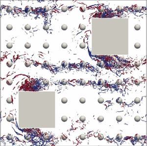
The instantaneous velocity magnitude in a cross-section for different values of porosity  ${\phi _s}$ is shown in figure 10. The Reynolds number $R{e_l}$ is 5060 for ${\phi _s} = 0.93$, which is much higher than the critical value of $R{e_l}$ for the onset of macroscopic turbulence when the porous matrix has only large porous elements. The value of $R{e_K}$ is 1302, suggesting that the flow is in the Forchheimer regime. However, no macroscopic turbulence is found in this case, see figure 10(a), while the microscopic turbulence is modelled. The macroscopic turbulence survives as the porosity ${\phi _s}$ is increased to 0.98 (figure 10b). Similarly, macroscopic turbulence is also found as ${\phi _s}$ is further increased, see figure 10(c) for ${\phi _s} = 0.99$ and figure 10(d) for ${\phi _s} = 1$. The macroscopic simulation results are consistent with the DNS results.

Figure 10. Instantaneous velocity magnitude, ‘bars+spheres’ with (a)  ${\phi _s} = 0.93$, $Da = 0.07$, $R{e_K} = 1302$, $R{e_l} = 5060$; (b) ${\phi _s} = 0.98$, $Da = 0.39$, $R{e_K} = 1225$, $R{e_l} = 1969$; (c) ${\phi _s} = 0.99$, $\; Da = 1.26$, $R{e_K} = 1135$, $R{e_l} = 1009$; (d) ${\phi _s} = 1.0$, $R{e_l} = 630$.
Figure 11 shows the turbulent two-point correlation  ${\hat{R}_{11}}(\boldsymbol{r},{\boldsymbol{x}_0})$ calculated from the macroscopic simulation. The test cases have similar values of $R{e_K}$. Now ${\hat{R}_{11}}(\boldsymbol{r},{\boldsymbol{x}_0})$ is equal to zero when ${\phi _s} = 0.93$ but has a non-zero range when ${\phi _s} \ge 0.98$. This non-zero range of ${\hat{R}_{11}}(\boldsymbol{r},{\boldsymbol{x}_0})$ exceeds $[ - {\textstyle{1 \over 4}}{s_l},{\textstyle{1 \over 4}}{s_l}]$, which corresponds to the microscopic length scale, and becomes wider as ${\phi _s}$ is increased from 0.98 to 1.

Figure 11. Turbulent two-point correlations in the streamwise ( ${x_1}$) direction (a) and transverse ( ${x_2}$) direction (b), ‘bars+spheres’.
Figure 12 shows the relationship between the Reynolds number  $R{e_K}$ and the normalized macroscopic turbulence kinetic energy $2\langle k\rangle /u_m^2$ for ${\phi _s} = 0.98$ and different $Da$ values. The onset of macroscopic turbulence occurs at $R{e_K} = 133$ for $Da = 0.39$ or $R{e_K} = 120$ for $Da = 0.10$. The results are consistent with the statement by Nield & Bejan (Reference Nield and Bejan2017) that the transition from a Darcy flow to a Darcy–Forchheimer flow occurs when $R{e_K}$ is of order ${10^2}$. In addition, we have found that the values of $2\langle k\rangle /u_m^2$ change only marginally when the $R{e_K}$ is above $1000$.

Figure 12. Normalized macroscopic turbulence kinetic energy  $2\langle k\rangle /u_m^2$ versus Reynolds number $R{e_K}$, ${\phi _s} = 0.98$, ‘bars+spheres’.
The longitudinal integral length scales  ${L_x}$ and ${L_y}$ for $R{e_K} > 1000$ are shown in figure 13. The macroscopic results are compared with the DNS results for ‘bars’. Both macroscopic simulation and DNS results show that ${L_x}$ and ${L_y}$ change only marginally when the value of $R{e_K}$ is increased. The values of ${L_x}$ and ${L_y}$ increase with the increase of ${\phi _s}$ and approach the values for ${\phi _s} = 1$. The macroscopic simulation results of $\langle {L_x}\rangle $ and $\langle {L_y}\rangle $ for ${\phi _s} = 1$ are 0.45 and 0.54, respectively, which are close to DNS results for ‘bars’.

Figure 13. Turbulent two-point correlations in the streamwise ( ${x_1}$) direction and transverse ( ${x_2}$) direction, ‘bars+spheres’ with (a) $\; {L_x}$; (b) ${L_y}$.
Figure 14 shows the premultiplied energy spectra of macroscopic simulation results. A plateau of  ${k_1}{\hat{E}_{11}}/u^{\prime2}_1 \approx 0.35$ can be found for porosity ${\phi _s} = 1$, which indicates the range of large-scale turbulent motion. The peak of ${k_1}{\hat{E}_{11}}$ for ${\phi _s} = 1$ corresponds to the wavelength ${\varLambda} = 1.33{s_l}$, which is identical to the value of $\varLambda $ for ${\phi _s} = 0.99$. When the porosity ${\phi _s}$ is decreased to 0.98, the value of $\varLambda $ declines to ${s_l}$ which is identical to the large pore size.

Figure 14. Premultiplied energy spectra for ‘bars+spheres’. The peaks with the lowest wavenumbers are indicated with solid circles.
The macroscopic simulation results discussed above are for a GPM made of spherical porous elements with the scale ratio  ${s_l}/{s_s} = 4$ or 8. The permeability K is calculated using the Carman–Kozeny equation (3.10). However, the values of K and the Darcy numbers calculated from this equation might have uncertainties due to the variation of the pore-scale geometries. To better understand the dependence of the critical porosity ${\phi _c}$ on the Darcy number, we have solved (3.13) and (3.14) with the drag terms expressed by (3.17) and (3.18) for different Darcy numbers. The solutions are independent of the Reynolds numbers. Figure 15 shows the relationship between ${\phi _s}$ and $2\langle k\rangle /u_m^2$. The macroscopic simulation results indicate that the critical porosity ${\phi _c}$ for the survival of macroscopic turbulence is between 0.95 and 0.97, which is similar to the DNS results. Now ${\phi _c}$ is not sensitive to the Darcy number when it is in the range 0.3–1.2. When ${\phi _s}$ is smaller than ${\phi _c}$, macroscopic turbulence cannot be stimulated even if $R{e_l} \to \infty $.

Figure 15. Normalized macroscopic turbulence kinetic energy  $2\langle k\rangle /u_m^2$ versus porosity. Here $R{e_l} \to \infty $, $Da \in [0.3,1.2]$, ‘bars+GPM’.
5. Conclusions
In order to understand whether macroscopic turbulence might survive in certain conditions and thus know the valid domain of the PSPH, we have studied the turbulent flows in porous matrices which have one or two length scales using DNS and macroscopic simulation. The large porous elements are made of two-dimensional bars with the element size  ${d_l}$ and spacing ${s_l}$, while the small porous elements are made of spheres or cubes with the element size ${d_s}$ and spacing ${s_s}$.
Instantaneous Q isosurfaces, turbulent two-point correlations, integral length scales and premultiplied energy spectra which are obtained from both DNS and macroscopic simulation are used to detect the possible macroscopic turbulence. The DNS results show that the critical porosity  ${\phi _c}$ for the survival of macroscopic turbulence is between 0.93 and 0.98 when the scale ratio ${s_l}/{s_s}$ is set to 4. When the porosity is lower than ${\phi _c}$, the integral length scales for porous matrices with two length scales (‘bars+spheres’ or ‘bars+cubes’) are almost identical to those for porous matrices with only small porous elements (‘spheres’ or ‘cubes’). When the flow is fully turbulent, the value of ${\phi _c}$ does not change markedly as the Reynolds number ( $R{e_s}$ or $R{e_l}$) is increased or the pore-scale elements are changed from ‘spheres’ to ‘cubes’.
The generality of the value of  ${\phi _c}$ is further studied using macroscopic simulation. The porous matrix made of spherical elements is modelled as a continuous porous medium whose geometric parameters are determined empirically. The macroscopic simulation results for ‘bars+spheres’ show that ${\phi _c}$ is in the range 0.95–0.97, which is close to the DNS results. Then, the macroscopic simulations for $R{e_l} \to \infty $ and the Darcy number values in the range 0.3–1.2 are performed. The numerical results show that ${\phi _c}$ is still in the range 0.95–0.97. It should be noted that that ${c_{B2}}$ for our macroscopic simulation is calculated using (3.12) and the coefficient of the Forchheimer term is set to ${c_{F1}} = 0.1$. The current critical porosity value ${\phi _c}$ is calculated based on the coefficient ${c_{B2}}$ and ${c_{F1}}$ values. When the Darcy number approaches zero, the macroscopic turbulence might survive only with larger critical porosity since the drag term becomes infinity in (3.17). The effect of pore-scale geometries on these coefficients has not been taken into account in our study. In addition, the DNS is for only two pore-scale geometries (‘spheres’ and ‘cubes’). The dependence of the critical porosity on the pore-scale geometry still needs to be further investigated.
The comparison between the DNS and macroscopic simulation results also confirms the accuracy of the PSPH model proposed by Rao et al. (Reference Rao, Kuznetsov and Jin2020), as well as the capability of using this model to directly resolve the macroscopic turbulence in porous media.
Acknowledgements
The authors gratefully acknowledged the support of this study by China Scholarship Council (CSC). Acknowledgment is also given to Professor M. Avila for the illuminating discussion with him. All parallel computations are performed using the cluster of the Center of Applied Space Technology and Microgravity (ZARM), University of Bremen.
Declaration of interests
The authors report no conflict of interest.
Appendix A. Verification and validation
The accuracy of the DNS solution can be examined by an accuracy measure, which we define as
 \begin{equation}\varDelta = \frac{{{g_1} - {g_s}}}{{{g_1}}},\end{equation}
where  ${g_1}$ and ${g_s}$ are the pressure gradient in the streamwise direction and the volume-averaged dissipation rate in the computational domain. Jin et al. (Reference Jin, Uth, Kuznetsov and Herwig2015) suggested that a solution with $\varDelta $ values below 10% for this type of flows is accurate enough for the analysis. Table 3 shows the values of $\varDelta $ for typical DNS cases.
Table 3. Main parameters for the typical DNS cases, LBM.

The FVM and LBM methods have been intensively applied and verified in our previous studies, see Jin et al. (Reference Jin, Uth, Kuznetsov and Herwig2015), Uth et al. (Reference Uth, Jin, Kuznetsov and Herwig2016), Jin & Kuznetsov (Reference Jin and Kuznetsov2017) and Rao et al. (Reference Rao, Kuznetsov and Jin2020). Here we make further verification using the cases in this study. Figure 16 shows the relationship between  $R{e_l}$ and the drag coefficient ${f_D} = {d_l}{g_1}/u_m^2$ calculated from different mesh resolutions and solvers (the FVM and the LBM). The porous matrix is made of staggered arrays of bars. It can be seen that calculated $R{e_l}$ is only marginally changed as the number of mesh cells is increased. The LBM results for the applied pressure gradient are approximately 6% higher than the FVM results. The reason is that the bounced back model used in the LBM leads to slightly larger solid region; this is an acknowledged error. Figures 17 and 18 show the LBM and FVM results for the two-point correlations and the premultiplied energy spectra; the marginal difference does not affect our analysis.

Figure 16. Applied pressure gradient  ${g_1}$ versus Reynolds number $R{e_l}$, DNS results. The porous matrix is made of staggered arrays of bars. Here FVM and LBM results with different mesh resolutions are compared.

Figure 17. Turbulent two-point correlations in the streamwise ( ${x_1}$) direction (a) and transverse ( ${x_2}$) direction (b). The porous matrix is made of staggered arrays of bars. Here FVM and LBM results are compared.

Figure 18. Premultiplied energy spectra. The porous matrix is made of staggered arrays of bars. Here FVM and LBM results are compared.
The cases ‘bars+spheres’ with  ${\phi _s} = 0.70$ are calculated using both DNS and macroscopic simulation methods. Figure 19 shows the time-, REV- and spanwise ( ${x_3}$) averaged velocity components ${\langle {\bar{u}_1}\rangle ^{v,{x_3}}}$ and ${\langle {\bar{u}_2}\rangle ^{v,{x_3}}}$ along the streamwise ( ${x_1}$) lines. It can be seen that the macroscopic simulation results are in reasonable accordance with the DNS results; the macroscopic simulation model is well validated.

Figure 19. Distribution of  ${\langle {\bar{u}_1}\rangle ^{v,{x_3}}}$ and ${\langle {\bar{u}_2}\rangle ^{v,{x_3}}}$ along the streamwise ( ${x_1}$) lines at ${x_2}/{s_s} = 0.5$ (squares), 2.5 (circles), 4.5 (up-pointing triangles) and 6.5 (down-pointing triangles). Solid symbols indicate DNS results and hollowed symbols indicate macroscopic simulation results. The porous matrix is ‘bars+spheres’ with ${\phi _s} = \; 0.70$. The Reynolds number $R{e_s}$ is 436 (a,b) or 620 (c,d).


 Open access