


1. Introduction
Viscoplastic materials are a branch of non-Newtonian fluids showing a threshold for the applied stress, called the yield stress. For applied stresses larger than the yield stress, the material deforms as a viscous fluid; when the applied stresses are smaller than the yield stress, the material behaves as a rigid solid (Bonn et al. Reference Bonn, Denn, Berthier, Divoux and Manneville2017). In this context, the term ‘viscoplastic materials’ refers typically to those that exhibit only viscous and plastic properties. On the other hand, as discussed in detail by Thompson, Sica & de Souza Mendes (Reference Thompson, Sica and de Souza Mendes2018), the term ‘yield stress materials’ may refer to those that show additional properties beside the yield stress threshold, such as elasticity, thixotropy and so on. There are many fluids with proven yield stress behaviour, including waxy crude oils, foamed cement and cement slurries, many food products (e.g. chocolate cream and jam), cosmetic products (e.g. moisturizing cream) and so on (Balmforth, Frigaard & Ovarlez Reference Balmforth, Frigaard and Ovarlez2014). Biological materials (e.g. mucus and mammalian blood) also exhibit the yield stress rheology, suggesting new problems in physiological sciences, biomedical applications and microfluidic technologies (Balmforth et al. Reference Balmforth, Frigaard and Ovarlez2014; Burinaru et al. Reference Burinaru, Avram, Avram, Marculescu, Tincu, Tucureanu, Matei and Militaru2018; Horner, Wagner & Beris Reference Horner, Wagner and Beris2021).
Superhydrophobic (SH) surfaces are created via adding micro- and nano-scale protrusions onto hydrophobic surfaces, in order to decrease the surface wettability and, hence, improve the slippery motion (Koch & Barthlott Reference Koch and Barthlott2009). Groovy structures are among most well-known protrusions, experimentally created on hydrophobic surfaces (Lee, Choi & Kim Reference Lee, Choi and Kim2016), allowing us to trap gas (usually air), causing a fluid slippage on these surfaces (Rothstein Reference Rothstein2010; Lee et al. Reference Lee, Choi and Kim2016). Considering an SH wall, the condition at which air is trapped between the liquid and the groovy wall is called the Cassie state. However, in some conditions, the trapped air escapes and the liquid penetrates into the groove, fills the cavity and forms the Wenzel state (Lee et al. Reference Lee, Choi and Kim2016; Hardt & McHale Reference Hardt and McHale2022). In this context, there are several possible scenarios for the liquid/air interface, summarized as follows: (i) the liquid/air interface is nearly flat and pinned at the edges of the groove (ideal Cassie state) (Hodes et al. Reference Hodes, Kirk, Karamanis and MacLachlan2017; Arenas et al. Reference Arenas, García, Fu, Orlandi, Hultmark and Leonardi2019; Tomlinson & Papageorgiou Reference Tomlinson and Papageorgiou2022); (ii) the interface is deformed towards the groove or towards the main flow while it is pinned at the groove edges (Crowdy Reference Crowdy2017b; Game, Hodes & Papageorgiou Reference Game, Hodes and Papageorgiou2019); (iii) the liquid partially fills the groove and the liquid/air interface is in contact with the side and bottom walls of the groove (and the interface is not anymore pinned to the groove edges) (Giacomello et al. Reference Giacomello, Chinappi, Meloni and Casciola2012; Papadopoulos et al. Reference Papadopoulos, Mammen, Deng, Vollmer and Butt2013; He et al. Reference He, Zhang, Wang, Wang, Yang, Wang and Lee2021). The occurrence of these situations is mostly dependent on the flow parameters and the surface properties, including the system pressure, surface tension and the fluid's rheology (Tsai et al. Reference Tsai, Peters, Pirat, Wessling, Lammertink and Lohse2009; Papadopoulos et al. Reference Papadopoulos, Mammen, Deng, Vollmer and Butt2013; Annavarapu et al. Reference Annavarapu, Kim, Wang, Hart and Sojoudi2019; Rofman et al. Reference Rofman, Dehe, Frumkin, Hardt and Bercovici2020; He et al. Reference He, Zhang, Wang, Wang, Yang, Wang and Lee2021).
Several experimental studies (Manukyan et al. Reference Manukyan, Oh, Van Den Ende, Lammertink and Mugele2011; Papadopoulos et al. Reference Papadopoulos, Mammen, Deng, Vollmer and Butt2013) have found large deformations and deflections of the liquid/air interface at the SH wall. However, in several other experiments, small values for the deflection of the liquid/air interface have been reported (Ou, Perot & Rothstein Reference Ou, Perot and Rothstein2004; Ou & Rothstein Reference Ou and Rothstein2005; Kirk, Hodes & Papageorgiou Reference Kirk, Hodes and Papageorgiou2017). In a series of experiments conducted by Ou et al. (Reference Ou, Perot and Rothstein2004), the pressure drop and flow rate have been measured for a pressure-driven flow through a microchannel with one SH wall decorated with cubic micro-posts ( $30$
$30$  $\mathrm {\mu }$m tall, $30$
$30$  $\mathrm {\mu }$m thick and spaced at $30$
$30$  $\mathrm {\mu }$m), with the channel height varying between 76 and 257 $\mathrm {\mu }$m. They have found the maximum deflection to be ${\sim }3$ $\mathrm {\mu }$m for the liquid/air interface, i.e. relatively small compared with the period of the micro-posts (which is $60$
$60$  $\mathrm {\mu }$m). Presenting a universal law, Annavarapu et al. (Reference Annavarapu, Kim, Wang, Hart and Sojoudi2019) have demonstrated that the shape and geometry of the SH microstructures can affect the deflection of the liquid/air interface. They have shown that the deflection of the liquid/air interface is proportional to the second power of the microstructure edge to the edge length. They have also proven that the critical Laplace pressure at which the wetting transition occurs changes with the microstructure geometry and shape (Annavarapu et al. Reference Annavarapu, Kim, Wang, Hart and Sojoudi2019). In particular, the Cassie state can be stabilized with having larger microstructure depths and smaller widths of the liquid/air interface (smaller slip area fractions) (He, Patankar & Lee Reference He, Patankar and Lee2003; Zhao & Yuan Reference Zhao and Yuan2015; Annavarapu et al. Reference Annavarapu, Kim, Wang, Hart and Sojoudi2019). In another series of studies, the channel height has been carefully adjusted to maintain a flat liquid/air interface in molecular dynamics simulations (Bao, Priezjev & Hu Reference Bao, Priezjev and Hu2020; Ren et al. Reference Ren, Hu, Bao, Zhang, Wen and Xie2021). Using certain microtrench SH surfaces, the Cassie state has been stabilized for turbulent flows (Xu et al. Reference Xu, Grabowski, Yu, Kerezyte, Lee, Pfeifer and Kim2020, Reference Xu, Yu, Kim and Kim2021). In addition, Choi et al. (Reference Choi, Kang, Park, Jeong and Lee2021) have proposed flexible overhangs of re-entrant structures to stabilize the Cassie state. Also, Zhang et al. (Reference Zhang, Klittich, Gao and Dhinojwala2017) have tuned the roughness of a carbon nanotube surface, producing a new surface showing SH properties with a stable Cassie state. It has also been demonstrated that SH surfaces with low intrinsic wettability show high resistance to the undesired Wenzel state; this is due to a weak attractive force between the fluid molecules and the substrate atoms (Verplanck et al. Reference Verplanck, Galopin, Camart, Thomy, Coffinier and Boukherroub2007; Zhang, Wang & Wang Reference Zhang, Wang and Wang2019). These recent studies have demonstrated the important role of the shape and geometry of the microstructures, the surface intrinsic wettability and the channel height for confined flows in controlling the deflection of the liquid/air interface and maintaining a stable Cassie state.
Considering numerous applications of SH surfaces in microfluidic technology (Belyaev & Vinogradova Reference Belyaev and Vinogradova2010; Tsai Reference Tsai2013; Lee et al. Reference Lee, Choi and Kim2016; Qi et al. Reference Qi, Niu, Ruck and Zhao2019), in some scenarios, the rheology of fluids flowing in microfluidic devices exhibits yield stress characteristics (Burinaru et al. Reference Burinaru, Avram, Avram, Marculescu, Tincu, Tucureanu, Matei and Militaru2018; Gao et al. Reference Gao2020). For example, human blood is a prevalent fluid synthesized in microfluidic devices, e.g. for disease diagnosis (Choi et al. Reference Choi, Ng, Fobel and Wheeler2012; Burinaru et al. Reference Burinaru, Avram, Avram, Marculescu, Tincu, Tucureanu, Matei and Militaru2018). Human blood's yield stress originates from complex interactions between red blood cells, leading to the formation of a three-dimensional network of rouleaux at low shear rates. Rouleaux formation and break up is also responsible for blood's thixotropy (Giannokostas et al. Reference Giannokostas, Moschopoulos, Varchanis, Dimakopoulos and Tsamopoulos2020, Reference Giannokostas, Dimakopoulos, Anayiotos and Tsamopoulos2021; Beris et al. Reference Beris, Horner, Jariwala, Armstrong and Wagner2021; Horner et al. Reference Horner, Wagner and Beris2021). New rheometers have been designed by the use of microfluidic technologies, e.g. to analyse the rheology of concentrated solutions of microgel particles in microchannels involving a yield stress (Nghe et al. Reference Nghe, Terriac, Schneider, Li, Cloitre, Abecassis and Tabeling2011).
Let us briefly mention some of the existing studies on viscoplastic fluid flows with homogeneous slip boundary conditions, which can occur on a hydrophobic or hydrophilic surface, assuming that the viscoplastic fluid slides on the solid wall. The flow of Herschel–Bulkley fluids in channels with wall slip has been analytically studied for symmetric (Ferrás, Nóbrega & Pinho Reference Ferrás, Nóbrega and Pinho2012) and asymmetric (Panaseti & Georgiou Reference Panaseti and Georgiou2017; Panaseti et al. Reference Panaseti, Vayssade, Georgiou and Cloitre2017) slip configurations. These works have analysed the viscoplastic fluid velocity profile using different slip models, including the linear and nonlinear Navier, empirical asymptotic and Hatzikiriakos slip models. The axial flow of a Bingham fluid through concentric annulus with wall slip has been analytically addressed by Kalyon & Malik (Reference Kalyon and Malik2012). Taghavi (Reference Taghavi2018) has studied multilayer flows of viscoplastic fluids in a narrow channel with symmetric and asymmetric wall slip conditions, evaluating the role of the different slip configurations on the overall flow picture. The stability of plane Poiseuille flow of Bingham fluids with wall slip has been recently studied, revealing stabilizing and destabilizing effects of the streamwise and spanwise slip conditions, respectively (Rahmani & Taghavi Reference Rahmani and Taghavi2020).
Regardless of the boundary conditions (e.g. slip or no slip), viscoplastic fluid flows are numerically studied using two main approaches i.e. the regularization and augmented Lagrangian methods, both of which are typically implemented in finite element/volume discretizations (Saramito & Wachs Reference Saramito and Wachs2017). Knowing the fact that, for an ideal viscoplastic fluid, the effective viscosity becomes infinite at the yield surface and within the plug, in the regularization approach the infinite viscosity is replaced by a very high value, following a viscosity function (Frigaard Reference Frigaard2019; Wachs Reference Wachs2019), e.g. as implemented in the well-known Papanastasiou regularization model (Putz, Frigaard & Martinez Reference Putz, Frigaard and Martinez2009). In the augmented Lagrangian method, on the other hand, the motion equations are formulated based on variational calculus and the flow solution is determined via an optimization algorithm (Saramito & Roquet Reference Saramito and Roquet2001). The augmented Lagrangian method has been enhanced in recent years to provide a faster solution convergence (Saramito Reference Saramito2016; Treskatis, Moyers-González & Price Reference Treskatis, Moyers-González and Price2016; Dimakopoulos et al. Reference Dimakopoulos, Makrigiorgos, Georgiou and Tsamopoulos2018). For instance, a fast converging and efficient algorithm based on a monolithic Newton solver for the augmented Lagrangian is proposed by Dimakopoulos et al. (Reference Dimakopoulos, Makrigiorgos, Georgiou and Tsamopoulos2018) and tested via solving for five benchmark problems. Recently proposed accelerated augmented Lagrangian methods have been evaluated by Treskatis et al. (Reference Treskatis, Roustaei, Frigaard and Wachs2018) and practical guides for efficient simulation of viscoplastic fluid flows have been presented.
While the augmented Lagrangian method is more accurate in capturing yield surfaces (Putz et al. Reference Putz, Frigaard and Martinez2009; Balmforth et al. Reference Balmforth, Frigaard and Ovarlez2014), the regularization method is generally faster (Muravleva et al. Reference Muravleva, Muravleva, Georgiou and Mitsoulis2010; Dimakopoulos, Pavlidis & Tsamopoulos Reference Dimakopoulos, Pavlidis and Tsamopoulos2013; Saramito & Wachs Reference Saramito and Wachs2017), making it suitable to deal with a large number of simulations. The Papanastasiou regularization model has been successfully used in numerous studies, e.g. to address the Poiseuille flow of viscoplastic fluids in ducts with wall slip (Damianou et al. Reference Damianou, Philippou, Kaoullas and Georgiou2014; Damianou & Georgiou Reference Damianou and Georgiou2014; Damianou, Kaoullas & Georgiou Reference Damianou, Kaoullas and Georgiou2016); in these works, the yield surfaces appearing at the centre and corners of the duct have been accurately captured.
The slip modelling for Newtonian fluid flows over SH groovy surfaces has been typically studied for two special cases, i.e. longitudinal and transverse groove configurations. In the former case, the flow direction is the same as that of the grooves and the effective slip length is given typically by  ${\hat {b}_{{eff}}^\parallel }$. However, in the transverse groove configuration, the flow direction is perpendicular to that of the grooves and the effective slip length is usually symbolized by ${\hat {b}_{{eff}}^\bot }$. For an ideal slippery condition on a liquid/gas interface (the Cassie state with no meniscus curvature), the pressure-driven flow has been studied by several researchers (Philip Reference Philip1972; Lauga & Stone Reference Lauga and Stone2003; Cottin-Bizonne et al. Reference Cottin-Bizonne, Barentin, Charlaix, Bocquet and Barrat2004) and the effective slip length has been formulated as $\hat {b}_{{eff}}^ \bot = ({\hat {L}}/{{2{\rm \pi} }})\ln [\sec({\rm \pi} \varphi/2)]$ (Belyaev & Vinogradova Reference Belyaev and Vinogradova2010), where ${\hat {L}}$ is the periodicity length of the grooves and ${{\varphi }}$ is the fraction of the liquid/gas interface. A more realistic model called the gas cushion model has been originally presented by Vinogradova (Reference Vinogradova1995) to predict the local slip at the slipping area (i.e. the liquid/gas interface), in the form of $\hat {b} = \hat {e}( {{\hat {\mu } }/{{{\hat {\mu } _a}}} - 1} ) \approx \hat {e}({\hat {\mu }}/{{{\hat {\mu }_a}}})$, where ${\hat {e}}$ is the gas layer thickness, and ${\hat {\mu }}$ and ${\hat {\mu }_a}$ represent the liquid and gas viscosities, respectively. An effective slip length model for the pressure-driven flow of Newtonian fluids over rectangular stripes has been presented by Belyaev & Vinogradova (Reference Belyaev and Vinogradova2010), solving the Poisson and Laplace equations for the slip-induced perturbations of the streamfunction and vorticity, respectively, leading to formulas for the longitudinal and transverse slip lengths. The limits of thick and thin channels have been considered in the modelling of flows over groovy surfaces, albeit mainly for Newtonian fluids. For thick channels, Asmolov et al. (Reference Asmolov, Zhou, Schmid and Vinogradova2013b) have developed an effective slip length model for a Newtonian shear-driven flow over weakly slipping rectangular stripes. Assuming the local slip length to be small in comparison with the scale of the heterogeneities, they have perturbed the Stokes equation, considered a linear Navier slip model, and developed a Fourier series solution for the perturbation velocity, eventually allowing them to calculate the slip velocity and lengths using a stick–slip boundary condition. Schmieschek et al. (Reference Schmieschek, Belyaev, Harting and Vinogradova2012) have generalized a tensorial effective slip theory, initially developed for thick channels, to any channel thickness. They have considered an asymmetric flow (i.e. no slip at the upper wall and groovy structures at the lower wall), along with the perturbed Stokes equation and the Navier slip law, as the governing equations; this has led to a Fourier series solution yielding trigonometric dual series (with exact solutions at the limit of thin and thick channels), describing the complete physics of the slip. Several other analytical efforts have been made to address the flow of Newtonian fluids over SH surfaces, to which an interested reader can refer (Asmolov & Vinogradova Reference Asmolov and Vinogradova2012; Asmolov et al. Reference Asmolov, Schmieschek, Harting and Vinogradova2013a; Schönecker, Baier & Hardt Reference Schönecker, Baier and Hardt2014; Asmolov, Nizkaya & Vinogradova Reference Asmolov, Nizkaya and Vinogradova2020).
Using computational fluid dynamics tools (e.g. in-house codes, Fluent, COMSOL Multiphysics, OpenFOAM, etc.), there are several numerical studies addressing the flow of Newtonian fluids over SH textures. For instance, Cheng, Teo & Khoo (Reference Cheng, Teo and Khoo2009) have addressed a pressure-driven flow through channels with SH surfaces (patterned with square posts), using a combined finite volume–finite difference method. Davies et al. (Reference Davies, Maynes, Webb and Woolford2006) have performed numerical simulations of the flow through microchannels with SH walls having transverse ribs, reporting a significant decrease in the frictional pressure drop and an increase in the slip velocity compared with the classical Poiseuille flow with smooth walls. Ou & Rothstein (Reference Ou and Rothstein2005) have analysed similar flows over SH surfaces, finding good agreement between the results of their numerical simulations and those of micro-particle image velocimetry experiments. Priezjev, Darhuber & Troian (Reference Priezjev, Darhuber and Troian2005) have simulated Newtonian Couette flow with an SH patterned stationary wall, using both the finite element method (for solving the Navier–Stokes equations) and the molecular dynamics method (to quantify the effective slip length). They have reported a reasonable agreement between the results of these simulation methods when the ratio of the slip region width to the molecular diameter is large. A few studies have also considered shear-thinning flows over SH surfaces. For instance, using the Carreau–Yasuda model, Patlazhan & Vagner (Reference Patlazhan and Vagner2017) have numerically studied the apparent slip of shear-thinning fluids in microchannels with SH groovy walls. They have simplified the flow into three regions, i.e. the core region as well as the stick and slip thin regions, each with a different viscosity, resulting in an estimation of the effective slip length. Haase et al. (Reference Haase, Wood, Sprakel and Lammertink2017) have performed numerical simulations of a pressure-driven flow of a shear-thinning fluid over a bubble mattress, representing an SH surface on which no-slip walls and no-shear gas bubbles are transversely positioned. They have found a general increase in the effective slip length for their shear-thinning fluid in comparison with a Newtonian fluid. In addition to the aforementioned numerical studies, there are several other works attempting to numerically model the slip phenomenon over SH surfaces using molecular dynamics simulations (Cottin-Bizonne et al. Reference Cottin-Bizonne, Barentin, Charlaix, Bocquet and Barrat2004), dissipative particle dynamics methods (Asmolov et al. Reference Asmolov, Zhou, Schmid and Vinogradova2013b) and lattice Boltzmann simulations (Schmieschek et al. Reference Schmieschek, Belyaev, Harting and Vinogradova2012).
Our brief review of the relevant studies so far has revealed that the literature of fluid flows over SH surfaces is well developed for Newtonian fluids, covering various flow scenarios and SH surface configurations, using analytical, numerical and experimental approaches. However, in spite of numerous applications of non-Newtonian fluids over SH surfaces (Crowdy Reference Crowdy2017a; Haase et al. Reference Haase, Wood, Sprakel and Lammertink2017; Kim et al. Reference Kim, Lee, Kim and Kwak2021), the relevant literature is limited only to a few shear-thinning fluid studies. In fact, to the best of our knowledge, the flow of viscoplastic materials over SH surfaces, as an important category of non-Newtonian fluids, has not yet been fundamentally studied, despite its existing and potential applications (Burinaru et al. Reference Burinaru, Avram, Avram, Marculescu, Tincu, Tucureanu, Matei and Militaru2018; Gao et al. Reference Gao2020; Ijaola, Farayibi & Asmatulu Reference Ijaola, Farayibi and Asmatulu2020; Li et al. Reference Li, Tian, Gao, Qin, Pi, Li and Yang2021). Via analysing plane Poiseuille flow of a Bingham fluid in a channel with an SH groovy lower wall, in the current work, we attempt to address this problem for the first time. In particular, assuming a flat liquid/air interface (i.e. the Cassie state), we develop a semi-analytical model based on considering infinitesimal wall-induced perturbations in the flow system and, then, solving the resulting equations using the Fourier series expansion method. We also use complementary OpenFOAM direct numerical simulations (DNSs), to validate our semi-analytical model results and elucidate the flow details and physics. Our analysis, including a combination of semi-analytical and DNS solutions, is fairly comprehensive, as it considers a range of thicknesses for thick channels and both creeping and inertial flow regimes, while providing regime classifications. In our analysis, the channel thickness is defined using the ratio between the dimensional values of the groove period ( $\hat L$) and the half-channel height ( $\hat H$, see figure 1); when $\hat H \gg \hat L$ the channel is assumed to be thick, while for $\hat H \ll \hat L$ the channel is thin.

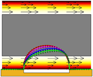
Figure 1. Schematic of the flow configuration. In this figure, dimensional geometrical parameters are shown. Here, and throughout the text, the dimensional parameters and variables are marked with ‘ $\hat {\ }$’ and the dimensionless ones without.
The outline of the present work is as follows. Section 2 introduces the governing equations of our flow system. In § 3, the semi-analytical model is first developed for the perturbation fields of the creeping and inertial flow regimes, for the thick channel limit. The total flow profile is then calculated at the end of this section. Section 4 presents the method for the complementary DNSs, including the numerical schemes and set-up (the computational mesh is presented in § 3 of online supplementary material available at https://doi.org/10.1017/jfm.2022.700). The results of our analysis are presented in § 5, for the thick channel limit (via the semi-analytical and DNS solutions). Afterwards, a criterion for the unyielded plug zone formation at the SH wall, followed by a regime classification, are presented. Finally, § 6 presents the summary and concluding remarks of the paper.
2. Governing equations
This section presents the governing equations for our plane Poiseuille flow of a Bingham fluid, in a two-dimensional (2-D) channel with an SH lower wall. This asymmetric flow configuration (with the lower boundary as an SH groovy wall and the upper wall with the no-slip condition) is studied due to practical considerations: in practice, a channel with two symmetrically aligned groovy walls (typically micro-nano sized grooves) is difficult to construct (Schmieschek et al. Reference Schmieschek, Belyaev, Harting and Vinogradova2012). At the SH wall, the transverse groovy structure is considered, while the main flow direction is normal to the groove direction. The schematic of the flow under study is presented in figure 1. Based on this figure,  $\hat L$ is the periodicity length of the grooves, $\hat \delta$ represents the width of the liquid/air interface, $\hat h$ and $\hat h^u$ are the SH wall distances from the lower and upper yield surfaces (i.e. the boundaries between the yielded zones and the unyielded centre plug zone), respectively, and $\hat H$ is the half-channel height. The coordinate origin is placed at the centre of the liquid/air interface on the SH wall.
The dimensionless continuity and momentum balance equations in two dimensions are presented as
 \begin{gather} \boldsymbol{\nabla} \boldsymbol{\cdot} {\boldsymbol{U}} = 0, \end{gather}
 \begin{gather}Re\left[ {\frac{{\partial {\boldsymbol{U}}}}{{\partial t}} + ( {{\boldsymbol{U}}\boldsymbol{\cdot} \boldsymbol{\nabla} } ) {\boldsymbol{U}}} \right] ={-} \boldsymbol{\nabla} P + \boldsymbol{\nabla} \boldsymbol{\cdot} {\boldsymbol{\tau }}, \end{gather}
where  $t$ is the time and ${\boldsymbol {U} = U {\boldsymbol {e}_x} + V {\boldsymbol {e}_y}}$ is the dimensionless velocity vector for which $U$ and $V$ are the velocity components in the $\boldsymbol {e}_x$ and $\boldsymbol {e}_y$ directions, respectively. In addition, the other variables are the pressure ( $P$) and the deviatoric stress tensor ( ${\boldsymbol {\tau }}$). To obtain the dimensionless form of the equations of motion, the half-channel height ( $\hat H$) has been considered as the characteristic length and the average velocity ( $\hat U_{ave}$) as the characteristic velocity; the pressure and stress fields have been made dimensionless using the characteristic viscous stress, i.e. $\hat \tau _{ch}=\hat \mu _p ({\hat U_{ave}}/{\hat H})$, where $\hat \mu _p$ is the plastic viscosity. Subsequently, the Reynolds number is defined as
 \begin{equation} {Re = \frac{{\hat \rho{{\hat U}_{ave}}\hat H}}{{{{\hat \mu }_p}}}}, \end{equation}
where  $\hat \rho$ is the fluid density.
To model the viscoplastic fluid rheology, the Bingham constitutive equation is used. The dimensionless form of the Bingham model is presented as
 \begin{equation}
\left. \begin{array}{c@{}} {\boldsymbol{\tau }} = \left( {1 +
\dfrac{Bi}{{\dot \gamma }}} \right) {\dot{\boldsymbol \gamma
}},\quad \tau > Bi,\\
\dot \gamma = 0, \quad \tau \le Bi,
\end{array} \right\}
\end{equation}
\begin{equation}
\left. \begin{array}{c@{}} {\boldsymbol{\tau }} = \left( {1 +
\dfrac{Bi}{{\dot \gamma }}} \right) {\dot{\boldsymbol \gamma
}},\quad \tau > Bi,\\
\dot \gamma = 0, \quad \tau \le Bi,
\end{array} \right\}
\end{equation}
where  ${\dot {\boldsymbol \gamma } = \boldsymbol {\nabla } \boldsymbol {u} + {( {\boldsymbol {\nabla } \boldsymbol {u}} )^T}}$ is the strain-rate tensor, and ${\tau = \sqrt {{{{\tau _{ij}}{\tau _{ij}}} /2}}}$ and ${\dot \gamma = \sqrt {{{{{\dot \gamma }_{ij}}{{\dot \gamma }_{ij}}}/2}}}$ are the magnitudes of the stress and strain-rate tensors, respectively. The Bingham number, representing the ratio of the yield stress ( ${{{\hat \tau _0}}}$) to the characteristic viscous stress ( $\hat \tau _{ch}$), is defined as
 \begin{equation} Bi = \frac{{{\hat \tau _0}\hat H}}{{{{\hat \mu }_p}{{\hat U}_{ave}}}}. \end{equation}
2.1. No-slip Poiseuille–Bingham flow profile
For a laminar 2-D channel Poiseuille flow with no-slip conditions at both walls, the flow pressure ( $P_0$) and velocity ( $U_0$) can be analytically obtained, by solving the dimensionless equations (2.1) and (2.2). Due to the symmetry with respect to the channel axis in the no-slip condition case, it suffices to derive the solution for the lower half of the channel
 \begin{gather} P_0 ={-} {\tau _w}x + \text{const.}, \end{gather}
 \begin{gather}{U_0}(y)=
\left\{ \begin{array}{@{}ll} {C_1}y + {C_2}{y^2}, & 0 \le y
\le {h}, \\ {C_3}, & {h} \le y \le 1, \end{array} \right.
\end{gather}
\begin{gather}{U_0}(y)=
\left\{ \begin{array}{@{}ll} {C_1}y + {C_2}{y^2}, & 0 \le y
\le {h}, \\ {C_3}, & {h} \le y \le 1, \end{array} \right.
\end{gather}
where  $C_1=\tau _w - Bi$, $C_2=-{\tau _w}/{2}$ and $C_3={(\tau _w - Bi)^2}/{2\tau _w}$. Here, $h$ is the location of the lower yield surface with respect to the lower wall. The wall shear stress, $\tau _w$ (at $y=0$), is the largest positive root of the following equation (refer to Frigaard & Ryan (Reference Frigaard and Ryan2004) for a similar equation):
 \begin{equation} 2\tau _w^3 - (3Bi + 6)\tau _w^2 + {Bi^3} = 0.\end{equation}
 After finding the wall shear stress ( $\tau _w$), the location of the lower yield surface ( $h$), representing the boundary between the lower yielded zone and the unyielded centre plug zone, can be calculated by
 \begin{equation} {{h} = 1 - \frac{Bi}{{{\tau _w}}}}.\end{equation}
2.2. Slip modelling
2.2.1. Slip origin
In our flow configuration, a layer of air trapped inside the wall grooves causes the bulk flow slippage on the liquid/air interface. On the other hand, the no-slip condition is considered for the liquid/solid contact at the SH wall and the upper wall. Shear stress at the flat liquid/air interface (i.e. the Cassie state assumption) is obtained as
 \begin{equation} {{\hat \tau _{la} = \hat \mu _a}\frac{{{{\hat u}_s}}}{{\hat \varepsilon }}},\end{equation}
where  $\hat \tau _{la}$ and ${{\hat u}_s}$ are the shear stress and the slip velocity at the liquid/air interface, respectively. Also, $\hat \mu _a$ is the dynamic viscosity of air and ${\hat \varepsilon }$ represents an average characteristic length for the air layer through which the air velocity reaches zero. Based on (2.10), the linear Navier slip law at the liquid/air interface is retrieved
 \begin{equation} {\hat u_s} = \hat b{\hat \tau _{la}},\quad {\rm{where}}\ \hat b = \frac{{\hat \varepsilon }}{{{{\hat \mu }_a}}}.\end{equation}
 In our study,  $\hat b$ is called the dimensional slip number and, as a parameter, it is generally dependent on the air flow dynamics inside the grooves. In particular, the slip number is strongly dependent on the value of $\hat \varepsilon$, while this value is under the influence of the Poiseuille flow dynamics inside the channel. To be more specific, the shear stress at the liquid/air interface affects the air flow dynamics inside the grooves; thus, it changes the values of $\hat \varepsilon$ and, eventually, the slip number. Considering a groove as a cavity inside which air flows, $\hat \varepsilon$ can be affected by the groove dimensions as well. Throughout our study, we simply work with the slip number and use a wide range of values for it, to be able to cover any possible scenario regarding the values/ranges of $\hat \varepsilon$.
2.2.2. Slip model
Considering the continuity of the shear stress at the liquid/air interface, we rewrite equation (2.11) based on the shear stress of the Bingham fluid at the liquid/air interface, i.e.  ${\hat \tau _{la}} = {\hat \mu _{la}}{\hat {\dot {\gamma }}_{xy}}$, to find the following equation:
 \begin{equation} \hat u_{s} = {\hat b}{\hat \mu_{la}}{\hat{\dot{\gamma}}_{xy}}, \end{equation}
where  ${\hat {\dot {\gamma }}_{xy}}$ is the flow shear strain rate at the liquid/air interface for the Bingham fluid. In addition, ${\hat \mu _{la}}$ is the general viscosity of the Bingham fluid at the liquid/air interface, defined as
 \begin{equation} {\hat \mu _{la}} = \left( {{{\hat \mu }_p} + \frac{{{{\hat \tau }_0}}}{{{{\hat{\dot{\gamma}}}_{la}}}}} \right), \end{equation}
where  ${\hat {\dot {\gamma }}_{la}}$ is the magnitude of the flow strain rate at the liquid/air interface (for the Bingham fluid). Substituting equation (2.13) into (2.12), the following relation is obtained:
 \begin{equation} {\hat u_s} = \hat b\left( {{{\hat \mu }_p} + \frac{{{{\hat \tau }_0}}}{{{{\hat{\dot{\gamma}} }_{la}}}}} \right){\hat{\dot{\gamma}} _{xy}}.\end{equation}
Making the above equation dimensionless, one can obtain
 \begin{equation} {u_s} = b\left( {1 + \frac{Bi}{{{{\dot \gamma }_{la}}}}} \right){\dot \gamma _{xy}},\end{equation}
where the dimensionless slip number,  $b$, is defined as:
 \begin{equation} b = {\frac{\hat b {\hat \mu }_p}{\hat H}}.\end{equation}
3. Semi-analytical model
In this section, our semi-analytical model is developed, at the steady-state condition, for plane Poiseuille flow of a Bingham fluid, considering an SH groovy lower wall. The model is developed for the flow in the thick channel limit, where the lower yield surface is assumed to be flat. The solution is obtained based on perturbing the lower yielded zone, via infinitesimal perturbations. Consequently, the perturbed governing equations for the lower yielded zone are solved. To be comprehensive and systematic, a semi-analytical model is first developed for the creeping flow regime (§ 3.1), where the inertial terms are negligible in the momentum balance equation. Then, the semi-analytical model is extended to include the inertial flow regime (§ 3.2), where a simplified version of the momentum balance equation is assumed to govern the flow physics. After presenting the perturbation fields in both creeping and inertial regimes, the total velocity profile is presented (§ 3.3). For the simplicity of the analysis, throughout our semi-analytical derivation, the Bingham fluid is assumed to have only a single unyielded region, i.e. the plug formed around the channel centreline. Therefore, the solutions derived in §§ 3.1 and 3.2 concern the yielded region only, while § 3.3 gives the total velocity for both yielded and unyielded regions.
3.1. Creeping flow
At small Reynolds numbers ( $Re \ll 1$), the momentum balance equation governs a creeping flow motion. The SH groovy wall induces infinitesimal perturbations in the flow, which eventually vanish at the lower yield surface (which is assumed to be flat for the thick channel limit). The flow field can be perturbed based on the no-slip Poiseuille flow, i.e. $\boldsymbol {U}=\boldsymbol {U}_0+\epsilon \boldsymbol {u}$ and $P=P_0 +\epsilon p$, where $\boldsymbol {u}$ and $p$ are the perturbation velocity and pressure, respectively, and $\boldsymbol {U}$ and $P$ are the total velocity and pressure, respectively. The perturbation velocity vector, i.e. $\boldsymbol {u}=u {\boldsymbol {e}_x}+v {\boldsymbol {e}_y}$, has two components in the $x$ and $y$ directions, i.e. $u$ and $v$, respectively. For the thick channel limit, the perturbation parameter can be defined as $\epsilon = \kappa ^{-1}$, where $\kappa$ is the wavenumber of the groovy SH wall ( $\kappa =2{\rm \pi} /\ell$ and $\ell =\hat L/\hat H$).
Considering infinitesimal wall-induced perturbations, an anisotropic perturbation stress tensor for the Bingham fluid can be derived, for which the components are shown at the leading order as (Frigaard, Howison & Sobey Reference Frigaard, Howison and Sobey1994; Nouar et al. Reference Nouar, Kabouya, Dusek and Mamou2007)
 \begin{gather} {\tau '_{ij}} = \mu ( \boldsymbol{U}_0 ){\dot \gamma _{ij}}( {\boldsymbol{u}} ) = \left( {1 + \frac{Bi}{{| {{{{{\rm d}{U_0}} /{{\rm d} y}}}} |}}} \right){\dot \gamma _{ij}} ( {\boldsymbol{u}} )\quad {\rm{if}}\ ij \ne xy,yx, \end{gather}
 \begin{gather}{\tau '_{ij}} = {\dot \gamma _{ij}}( {\boldsymbol{u}} )\quad {\rm{if}}\ ij = xy,yx, \end{gather}
where  $d$ is the ordinary derivative operator and $i,j$ refer to the components of the coordinate system.
Imposing infinitesimal wall-induced perturbations in the momentum balance equation and having the perturbation stress components for the Bingham fluid (shown in (3.1) and (3.2)), we can derive the perturbation equations in the  $x$ and $y$ directions. We should recall that the perturbation parameter is dropped in the obtained perturbation equations; thus, we do not consider it in the following formulations and calculations. Taking the curl of the perturbed equations and using the definition of the streamfunction for the perturbation field ( $u = {{\partial \psi }}/{{\partial y}}$ and $v = - {{\partial \psi }}/{{\partial x}}$), we obtain a fourth-order partial differential equation for the perturbation streamfunction
 \begin{equation} \frac{{{\partial^4}\psi }}{{\partial {x^4}}} + \frac{{{\partial^4}\psi }}{{\partial {y^4}}} + \left( {2 + \frac{{4Bi}}{{| {{{{\rm d}{U_0}} /{{\rm d} y}}} |}}} \right) \frac{{{\partial^4}\psi }}{{\partial {x^2}\partial {y^2}}} - 4Bi\frac{{{{{{\rm d}^2}{U_0}}/{{\rm d}{y^2}}}}}{{{{( {{{{\rm d}{U_0}} /{{\rm d} y}}} )}^2}}}\frac{{{\partial^3}\psi }}{{\partial {x^2} \partial y}} = 0.\end{equation}
 It is assumed that the perturbation field is periodic in the  $x$ direction, with the period of the SH wall, i.e. $\ell ={\hat L}/{\hat H}$; thus, the solution for the perturbation streamfunction can be written in a Fourier series form for the $x$ component
 \begin{equation} \psi (x,y) = \sum_{n ={-} \infty }^\infty {A_n}{\hat \psi } (n,y)\,{{\rm e}^{{\rm i}n\kappa x}}, \end{equation}
where  $\kappa ={2{\rm \pi} }/{\ell }$, representing the wavenumber for the SH groovy wall and $A_n$ are the unknown coefficients.
Before proceeding, note that in our analysis we have assumed that the period of the perturbed flow is the same as the period of the SH surface. This assumption follows several previous studies through the literature regarding the flow of Newtonian fluids over SH surfaces with periodic microstructures (Lauga & Stone Reference Lauga and Stone2003; Belyaev & Vinogradova Reference Belyaev and Vinogradova2010; Asmolov & Vinogradova Reference Asmolov and Vinogradova2012; Schmieschek et al. Reference Schmieschek, Belyaev, Harting and Vinogradova2012; Schnitzer & Yariv Reference Schnitzer and Yariv2017). However, we should also mention that this assumption may not be always valid. In other words, considering the flow period to be the same as the period of geometry is an assumption that requires further examination, e.g. through the Floquet–Bloch theory (Pettas et al. Reference Pettas, Karapetsas, Dimakopoulos and Tsamopoulos2019; Marousis et al. Reference Marousis, Pettas, Karapetsas, Dimakopoulos and Tsamopoulos2021; Rohan, Nguyen & Naili Reference Rohan, Nguyen and Naili2021).
Substituting equation (3.4) into (3.3), while substituting for  ${{{\textrm {d}{U_0}}/{\textrm {d}y}}}$ and ${{{{\textrm {d}^2}{U_0}}/{\textrm {d}{y^2}}}}$ from (2.7), we obtain a fourth-order ordinary differential equation for ${\hat \psi }$
 \begin{equation} \frac{{{{\rm d}^4}\hat \psi }}{{{\rm d}{y^4}}} - \left( {2 + \frac{{4Bi}}{{{C_1} + 2{C_2}y}}} \right){n^2}{\kappa^2} \frac{{{{\rm d}^2}\hat \psi }}{{{\rm d}{y^2}}} + 8Bi{n^2}{\kappa ^2}\frac{{{C_2}}}{{{{( {{C_1} + 2{C_2}y} )}^2}}} \frac{{{\rm d}\hat \psi }}{{{\rm d} y}} + {n^4}{\kappa ^4} \hat \psi = 0.\end{equation}
To close the boundary value problem, the following boundary conditions are considered ( $n \ne 0$):
 \begin{equation} \hat \psi (n,0) = 0,\quad \hat \psi (n,h) = 0,\quad \frac{{{\rm d}\hat \psi }}{{{\rm d} y}}(n,h) = 0,\quad \frac{{{{\rm d}^2}\hat \psi }}{{{\rm d} {y^2}}}(n,h) = 0. \end{equation}
 Let us clarify the boundary conditions introduced above in (3.6a–d), which are derived for non-zero modes of the Fourier expansion, i.e.  $n \ne 0$. Generally, the boundary conditions for our problem originate from the following: (i) the no-penetration condition at the SH wall (i.e. $v=0$ at $y=0$); (ii) the zero perturbation velocity at the lower yield surface, i.e. $u=0$ and $v=0$ at $y=h$ (Frigaard et al. Reference Frigaard, Howison and Sobey1994; Nouar et al. Reference Nouar, Kabouya, Dusek and Mamou2007); (iii) the slip–stick condition at the SH wall. For $n=0$, (3.5) reduces to ${{{\textrm {d}^4}\hat \psi }}/{{\textrm {d} {y^4}}}=0$, which has a quadratic function solution, the general form of which can be obtained using the no-penetration condition at $y=0$ and the zero perturbation velocities at ${y=h}$, as boundary conditions. The first condition in (3.6a–d) satisfies the no-penetration requirement at the SH wall for the non-zero Fourier terms. Since the zero-term solution of $\psi$ is only a function of $y$, the zero-term solution of $v$ is always zero. Therefore, the first condition that is applied to the non-zero Fourier modes is sufficient to satisfy the no-penetration requirement at the SH wall. In a same way, the second boundary condition ensures having $v=0$ at the lower yield surface. The third boundary condition also ensures a zero streamwise perturbation velocity ( $u=0$) at the lower yield surface. Finally, the fourth boundary condition implies that the perturbation field rapidly decays away from the SH wall in the $y$ direction for the flow in the thick channel limit, consistent with the assumption of a flat lower yield surface. In other words, assuming a flat lower yield surface and a zero strain-rate magnitude at the yield surface for the Bingham fluids (see (2.4)) implies that each single non-zero Fourier mode of the perturbation shear gradient at the lower yield surface must vanish (as the yield surface is flat and its location is independent of $x$).
$x$).
Equation (3.5) with the boundary conditions (3.6a–d) can be solved numerically for thick channels. For the numerical scheme, a system of nonlinear equations is set up and solved using a Runge–Kutta collocation method combined with a Newton method, which is a fourth-order integration scheme to solve boundary value problems. The bvp4c routine in MATLAB R2020a is used to implement the method and discretize our system of nonlinear equations. Note that, as explained further below, in our flow configuration,  $h$ is generally unknown and it is found based on an iterative method, using an initial value based on the no-slip Poiseuille–Bingham channel flow.
Considering  $\hat \psi _n (y) = f_n(y)$ (for $n > 0$) and combining the zero and non-zero Fourier mode solutions, we write the simplified closed form solution of the perturbation streamfunction and velocities as
 \begin{gather} \psi (x,y) = {A_0}\left( {y - \frac{{{y^2}}}{{2h}}} \right) + \sum_{n = 1}^\infty {{A_n}} {f_n}(y)\cos ( {n\kappa x} ), \end{gather}
 \begin{gather}u(x,y) = {A_0}\left( {1 - \frac{y}{h}} \right) + \sum_{n = 1}^\infty {{A_n}} {{f'_n}}(y)\cos ( {n\kappa x} ), \end{gather}
 \begin{gather}v(x,y) = \sum_{n = 1}^\infty {{A_n}n\kappa } {f_n}(y)\sin ( {n\kappa x} ), \end{gather}
where  $'$ denotes the first derivative with respect to $y$; also, $A_n (n=0,1,2,\ldots$) are unknown coefficients, which are obtained based on the slip–stick boundary condition.
The linear Navier slip law with a local slip number ( $b$) is considered for the liquid/air interface at the groovy wall, while the no-slip condition is assumed for the liquid/solid interface. Consequently, the following boundary conditions are obtained at the groovy wall:
 \begin{gather} {u}(x,0) - b{\left( {Bi + \frac{{{\rm d} {U_0}}}{{{\rm d} y}} + \frac{{\partial u}}{{\partial y}}} \right)_{y = 0}} = 0, \quad 0 \leq x \leq \frac{\varphi \ell}{2}, \end{gather}
 \begin{gather}{u}(x,0) = 0,\quad \frac{\varphi \ell}{2} \leq x \leq \frac{\ell}{2}, \end{gather}
where  $\varphi = {\hat \delta }/{\hat L}$ represents the fraction of one groove that is exposed to slip (also called the slip area fraction). Substituting equations (2.7) and (3.8) into (3.10) and (3.11), we have
 \begin{gather}
{A_0}\left( {1 + \frac{b}{h}} \right) + \sum_{n = 1}^\infty
{{A_n}} [ {{{f'_n}}(0) - b{{f''_n}}(0)} ]\cos ( {n\kappa x}
) = b( {Bi + {C_1}} ), \quad 0 \leq x \leq \frac{\varphi
\ell}{2}, \end{gather}
\begin{gather}
{A_0}\left( {1 + \frac{b}{h}} \right) + \sum_{n = 1}^\infty
{{A_n}} [ {{{f'_n}}(0) - b{{f''_n}}(0)} ]\cos ( {n\kappa x}
) = b( {Bi + {C_1}} ), \quad 0 \leq x \leq \frac{\varphi
\ell}{2}, \end{gather} \begin{gather}{A_0} +
\sum_{n = 1}^\infty {{A_n}} {{f'_n}}(0)\cos ( {n\kappa x} )
= 0, \quad \frac{\varphi \ell}{2} \leq x \leq
\frac{\ell}{2},
\end{gather}
\begin{gather}{A_0} +
\sum_{n = 1}^\infty {{A_n}} {{f'_n}}(0)\cos ( {n\kappa x} )
= 0, \quad \frac{\varphi \ell}{2} \leq x \leq
\frac{\ell}{2},
\end{gather}
where  $''$ refers to the second derivative with respect to $y$.
$y$.
Equations (3.12) and (3.13) represent a dual series problem and, in contrast to their corresponding dual series for Newtonian fluids in the thick and thin channel limits, they have no closed form solution in their present form (see Sneddon Reference Sneddon1966; Belyaev & Vinogradova Reference Belyaev and Vinogradova2010). However, (3.12) and (3.13) can be solved using a similar technique to that used in Schmieschek et al. (Reference Schmieschek, Belyaev, Harting and Vinogradova2012):
(i) Equation (3.12) is integrated in $[0\ x]$ and then multiplied by ${\sin }(m\kappa x)$, where $m$ is a positive integer. Afterwards, the obtained equation is integrated in $[0\ {\varphi \ell }/{2}]$.
(ii) Equation (3.13) is multiplied by
${\cos }(m\kappa x)$ and then integrated in $[{\varphi \ell }/{2}\ {\ell }/{2}]$.


Subsequently, a system of linear equations is obtained
 \begin{equation} \sum_{n = 0}^N {{P_{mn}}{A_n}} = {M_m},\end{equation}
in which  $A_n (n=0,\ldots,N$) are the unknown coefficients. The coefficient and constant matrices for (3.14) are obtained as follows:
 \begin{gather} {P_{m0}} = \left( {1 + \frac{b}{h}} \right)\int_0^{{\varphi \ell}/{2}} {x\sin (m\kappa x)\,{{\rm d}\,x} }+ \int_{{\varphi\ell}/{2}}^{{\ell}/{2}}{\cos (m\kappa x)\,{{\rm d}\,x}}, \end{gather}
 \begin{gather}{P_{mn}}
= \frac{1}{{n\kappa }}[ {{{f'_n}}(0) - b{{f''_n}}(0)} ]
\int_0^{{{\varphi \ell}}/{2}} \sin ( {n\kappa x} ) \sin
(m\kappa x)\,{{\rm d}\,x}\nonumber\\
\quad + {{f'_n}}(0)\int_{{{\varphi
\ell}}/{2}}^{{\ell}/{2}} {\cos ( {n\kappa x} )\cos (m\kappa
x)\,{{\rm d}\,x}},
\end{gather}
\begin{gather}{P_{mn}}
= \frac{1}{{n\kappa }}[ {{{f'_n}}(0) - b{{f''_n}}(0)} ]
\int_0^{{{\varphi \ell}}/{2}} \sin ( {n\kappa x} ) \sin
(m\kappa x)\,{{\rm d}\,x}\nonumber\\
\quad + {{f'_n}}(0)\int_{{{\varphi
\ell}}/{2}}^{{\ell}/{2}} {\cos ( {n\kappa x} )\cos (m\kappa
x)\,{{\rm d}\,x}},
\end{gather} \begin{gather}{M_m} = b( {Bi + {C_1}} )\int_0^{{\varphi \ell}/{2}} {x\sin (m\kappa x)\,{{\rm d}\,x}}. \end{gather}
 Solving the system of linear equations (3.14), we can calculate the unknown coefficients of the solution, i.e.  $A_n$. However, for our viscoplastic flow configuration, we need an extra iterative approach in order to calculate the location of the lower yield surface ( $h$), which is affected by the slip condition at the SH wall; as we increase the slip number, we may expect the yield surface to move towards the SH wall.
Considering the total flow obtained for the lower yielded zone, the magnitude of the strain rate is now calculated as
 \begin{equation} \dot \gamma = \sqrt {{{\left( {\frac{{\partial U}}{{\partial y}} + \frac{{\partial V}}{{\partial x}}} \right)}^2} + 4{{\left( {\frac{{\partial U}}{{\partial x}}}\right)}^2}},\end{equation}
where  $U=U_0+u$ and $V=v$.
According to the Bingham model, at the yield surface,  $\dot \gamma$ must vanish. Having zero perturbation velocities at the lower yield surface implies that ${{\partial U}/{\partial x}}$ and ${{\partial V}/{\partial x}}$ are always zero at $y=h$. Therefore, the only requirement at the yield surface is to have ${{\partial U}/{\partial y}}=0$. To obtain this, in every iteration we start the solution process from (3.5) and, after solving the followed system of linear equations (3.14), we then check for the new location of the yield surface (new $h$) at which ${{\partial U}/{\partial y}}=0$; we subsequently update the value of $h$. This iterative approach continues until reaching a converged value for $h$ such that $\left|{{h_{new}} - {h_{old}}}\right|<eps$. We realize that for $eps=10^{-6}$, only five to six iterations and for $eps=10^{-4}$ only two to three iterations are required in most cases to obtain the converged solution.
Before we proceed, let us note that certain flow assumptions may allow us to develop an approximate solution for the thick channel flows, presented in § 1 of the online supplementary material, for the sake of completeness of the current study.
3.2. Inertial flow
In this section, we extend the semi-analytical model to account for inertial flows in the thick channel limit. To do so, we take advantage of the same method developed for the creeping flow regime (§ 3.1) to calculate the perturbation field. Therefore, we again consider the solution to be a superposition of the no-slip profile and the infinitesimal perturbation field induced by the SH groovy wall. Perturbing equations (2.1) and (2.2) with infinitesimal wall-induced perturbations and solving for the leading-order terms (i.e. by ignoring the nonlinear perturbed advection terms), we end up with the following equation for the perturbation streamfunction in the ( $x,y$) coordinate:
 \begin{align} &Re\left( {{U_0}\left( {\frac{{{\partial^3}\psi }}{{\partial x\partial {y^2}}} + \frac{{{\partial^3}\psi }}{{\partial {x^3}}}} \right) - \frac{{{{\rm d}^2}{U_0}}}{{{\rm d} {y^2}}} \frac{{\partial \psi }}{{\partial x}}} \right) = \frac{{{\partial^4}\psi }}{{\partial {x^4}}} + \frac{{{\partial^4}\psi }}{{\partial {y^4}}}\nonumber\\ &\quad + \left( {2 + \frac{{4Bi}}{{| {{{{\rm d}{U_0}}/{{\rm d} y}}} |}}} \right)\frac{{{\partial^4}\psi }}{{\partial {x^2}\partial {y^2}}}- 4Bi\frac{{{{{{\rm d}^2}{U_0}}/{{\rm d} {y^2}}}}}{{{{({{{{\rm d}{U_0}} /{{\rm d} y}}})}^2}}}\frac{{{\partial^3}\psi }}{{\partial{x^2} \partial y}}. \end{align}
Assuming a periodic flow in the  $x$ direction (with the same period as that of the SH wall), we rely on a Fourier series solution in the form of (3.4). Therefore, (3.19) is converted to an ordinary differential equation
 \begin{align} &\frac{{{{\rm d}^4}\hat \psi }}{{{\rm d} {y^4}}} - \left[ {\left( {2 + \frac{{4Bi}}{{{C_1} + 2{C_2}y}}} \right){n^2}{\kappa ^2} + {\rm i}n\kappa Re ( {{C_1}y + {C_2}{y^2}} )} \right]\frac{{{{\rm d}^2}\hat \psi }}{{{\rm d} {y^2}}} \nonumber\\ &\quad + 8Bi{n^2}{\kappa ^2}\frac{{{C_2}}}{{{{( {{C_1} + 2{C_2}y} )}^2}}}\frac{{{\rm d} \hat \psi }}{{{\rm d} y}} + [{{n^4}{\kappa ^4} + i{n^3}{\kappa ^3}Re( {{C_1}y + {C_2}{y^2}} ) + i2n\kappa {C_2}Re} ]\hat \psi = 0. \end{align}
 Equation (3.20) together with the boundary conditions of (3.6a–d) is solved using the same algorithm explained earlier (see § 3.1). For  $n=0$, we have the same quadratic solution for $\hat \psi$ as in the previous section. For $n>0$, we assume that the solution of (3.20) can be written as $\hat \psi _n (y) = f_n(y) + i g_n(y)$; therefore, we obtain the function $\psi$
 \begin{align} \psi
(x,y) &= {A_0}\left( {y - \frac{{{y^2}}}{{2h}}} \right) +
\sum_{n = 1}^\infty {{A_n}( {{f_n}(y) + i{g_n}(y)} )}\,
{{\rm e}^{{\rm i} n\kappa x}}\nonumber\\
&\quad + \sum_{n = 1}^\infty {A_n^*[
{{f_n}(y) - i{g_n}(y)} ]} \,{{\rm e}^{ - {\rm i}n\kappa
x}}.\end{align}
\begin{align} \psi
(x,y) &= {A_0}\left( {y - \frac{{{y^2}}}{{2h}}} \right) +
\sum_{n = 1}^\infty {{A_n}( {{f_n}(y) + i{g_n}(y)} )}\,
{{\rm e}^{{\rm i} n\kappa x}}\nonumber\\
&\quad + \sum_{n = 1}^\infty {A_n^*[
{{f_n}(y) - i{g_n}(y)} ]} \,{{\rm e}^{ - {\rm i}n\kappa
x}}.\end{align}
The rightmost term in the right-hand side of (3.21) represents the negative modes of the Fourier series solution (see (3.4)), written for simplicity based on the positive values of  $n$. Based on this simplification, one can easily show that $A_n^*$ must be the complex conjugate of $A_n$. Therefore, the following solution can be derived for $\psi$:
 \begin{align} \psi (x,y) &= {A_0}\left( {y - \frac{{{y^2}}}{{2h}}} \right) + \sum_{n = 1}^\infty {A_n^r[ {{f_n}(y)\sin ( {n\kappa x} ) + {g_n}(y)\cos ( {n\kappa x} )} ]} \nonumber\\ & \quad + \sum_{n = 1}^\infty {A_n^i[ {{g_n}(y)\sin ( {n\kappa x} ) - {f_n}(y)\cos ( {n\kappa x} )} ]}, \end{align}
where  $A_0$, $A_n^r$ and $A_n^i$ are unknown coefficients. Therefore, the perturbation velocities ( $u,v$) are obtained as
 \begin{align} u(x,y)
&= {A_0}\left( {1 - \frac{y}{h}} \right) + \sum_{n =
1}^\infty {A_n^r[ {{{f'_n}}(y)\sin ( {n\kappa x} ) +
{{g'_n}}(y)\cos ( {n\kappa x} )} ]} \nonumber\\
&\quad + \sum_{n = 1}^\infty {A_n^i[ {{{g'_n}}(y)\sin ( {n\kappa x}
) - {{f'_n}}(y)\cos ( {n\kappa x} )} ]}.
\end{align}
\begin{align} u(x,y)
&= {A_0}\left( {1 - \frac{y}{h}} \right) + \sum_{n =
1}^\infty {A_n^r[ {{{f'_n}}(y)\sin ( {n\kappa x} ) +
{{g'_n}}(y)\cos ( {n\kappa x} )} ]} \nonumber\\
&\quad + \sum_{n = 1}^\infty {A_n^i[ {{{g'_n}}(y)\sin ( {n\kappa x}
) - {{f'_n}}(y)\cos ( {n\kappa x} )} ]}.
\end{align} \begin{align}
v(x,y) &= \sum_{n = 1}^\infty {A_n^rn\kappa [ {{g_n}(y)\sin (
{n\kappa x} ) - {f_n}(y)\cos ( {n\kappa x} )} ]}
\nonumber\\
& \quad - \sum_{n = 1}^\infty {A_n^in\kappa [{{g_n}(y)\cos (
{n\kappa x} ) + {f_n}(y)\sin ( {n\kappa x})}]}.
\end{align}
\begin{align}
v(x,y) &= \sum_{n = 1}^\infty {A_n^rn\kappa [ {{g_n}(y)\sin (
{n\kappa x} ) - {f_n}(y)\cos ( {n\kappa x} )} ]}
\nonumber\\
& \quad - \sum_{n = 1}^\infty {A_n^in\kappa [{{g_n}(y)\cos (
{n\kappa x} ) + {f_n}(y)\sin ( {n\kappa x})}]}.
\end{align} By comparing the streamwise perturbation velocity ( $u$) for the inertial flow regime, shown in (3.23), with the corresponding solution for the creeping flow regime, shown in (3.8), we can realize that the inertial effects (amplified by increasing $Re$) are responsible for an asymmetry of the velocity profile in $x \in [-{\ell }/{2} \ {\ell }/{2}]$; i.e. $u(x,y_0) \ne u(-x,y_0)$, where $y_0$ represents a fixed value of $y$. Consequently, we can separate the flow profiles into even and odd functions, in $x \in [-{\ell }/{2} \ {\ell }/{2}]$, which for the streamwise perturbation velocity leads to
 \begin{gather} {u_e}(x,y) = {A_0}\left( {1 - \frac{y}{h}} \right) + \sum_{n = 1}^\infty {[ {A_n^r{{g'_n}}(y) - A_n^i{{f'_n}}(y)} ]} \cos ( {n\kappa x} ), \end{gather}
 \begin{gather}{u_o}(x,y) = \sum_{n = 1}^\infty {[ {A_n^r{{f'_n}}(y) + A_n^i{{g'_n}}(y)} ]} \sin ( {n\kappa x} ), \end{gather}
where the subscripts  $e$ and $o$ refer to even and odd functions, respectively. Since the no-slip shear stress ( ${Bi + {{\textrm {d} {U_0}}}/{{\textrm {d} y}}}$) is always an even function in $x \in [-{\ell }/{2} \ {\ell }/{2}]$, we can write the Navier slip law separately for the even and odd contributions of the velocity profile as
 \begin{gather} {{u}_{e}}(x,0) - b{\left( {Bi + \frac{{{\rm d} {U_0}}}{{{\rm d} y}} + \frac{{\partial {{u}_{e}}}}{{\partial y}}} \right)_{y = 0}} = 0, \quad 0 \le x \le \frac{\varphi \ell}{2}, \end{gather}
 \begin{gather}{{u}_{e}}(x,0) = 0,\quad \frac{\varphi \ell}{2} \le x \le \frac{\ell}{2}. \end{gather}
 \begin{gather}{{u}_{o}}(x,0) - b{\left({\frac{{\partial {{u}_{o}}}}{{\partial y}}} \right)_{y = 0}} = 0,\quad 0 \le x \le \frac{\varphi \ell}{2}, \end{gather}
 \begin{gather}{{u}_{o}}(x,0)
= 0,\quad \frac{\varphi \ell}{2} \le x \le \frac{\ell}{2}.
\end{gather}
\begin{gather}{{u}_{o}}(x,0)
= 0,\quad \frac{\varphi \ell}{2} \le x \le \frac{\ell}{2}.
\end{gather}Substituting equations (3.25) and (3.26) in (3.27) to (3.30), we find
 \begin{gather}
{A_0}\left( {1 + \frac{b}{h}} \right) + \sum_{n = 1}^N {[ {A_n^r( {{{g'_n}}(0) - b{{g''_n}}(0)} ) -
A_n^i ( {{{f'_n}}(0) - b{{f''_n}}(0)})}]} \cos ({n\kappa x} )\nonumber\\
= b( {Bi + {C_1}} ),\quad 0 \le x \le \frac{{\varphi \ell}}{2},
\end{gather}
\begin{gather}
{A_0}\left( {1 + \frac{b}{h}} \right) + \sum_{n = 1}^N {[ {A_n^r( {{{g'_n}}(0) - b{{g''_n}}(0)} ) -
A_n^i ( {{{f'_n}}(0) - b{{f''_n}}(0)})}]} \cos ({n\kappa x} )\nonumber\\
= b( {Bi + {C_1}} ),\quad 0 \le x \le \frac{{\varphi \ell}}{2},
\end{gather} \begin{gather}0 = {{A_0} + \sum_{n = 1}^N {( {A_n^r{{g'_n}}(0) - A_n^i{{f'_n}}(0)} )} \cos ( {n\kappa x} ), \quad \frac{\varphi \ell}{2} \le x \le \frac{\ell}{2}}, \end{gather}
and
 \begin{gather} \sum_{n = 1}^N {[ {A_n^r( {{{f'_n}}(0) - b{{f''_n}}(0)} ) + A_n^i( {{{g'_n}}(0) - b{{g''_n}}(0)} )} ]} \sin ( {n\kappa x} ) = 0,\quad 0 \le x \le \frac{{\varphi \ell}}{2}, \end{gather}
 \begin{gather}\sum_{n = 1}^N {( {A_n^r{{f'_n}}(0) + A_n^i{{g'_n}}(0)} ) } \sin ( {n\kappa x} ) = 0, \quad \frac{\varphi \ell}{2} \le x \le \frac{\ell}{2}, \end{gather}
where the series are truncated to the  $N$th terms.
Based on (3.33) and (3.34), a relation between the coefficients  $A_n^r$ and $A_n^i$ is calculable. To do so, the same method as used in § 3.1 is employed: (3.33) is integrated with respect to $x$ in $[0 \; x]$ and, then, the resulting equation is multiplied with $\cos (m\kappa x)$ (where $m$ is a positive integer) and again integrated in $x \in [0 \ {\varphi \ell }/{2}]$. Equation (3.34) is multiplied by $\sin (m\kappa x)$ and, then, it is integrated in $x \in [{\varphi \ell }/{2} \ {\ell }/{2}]$. The combination of the resulting equations and some algebra leads to the following relation between the unknown coefficients:
 \begin{equation} A_m^i = \sum_{n = 1}^N {{{[ {{{( {{P^i}} )}^{ - 1}}{P^r}} ]}_{m,n}}A_n^r}, \end{equation}
where the matrices  $\boldsymbol{\mathsf{P}}^r$ and $\boldsymbol{\mathsf{P}}^i$ are obtained as:
 \begin{align} P_{mn}^r
&= \frac{{{1}}}{n\kappa}( {{{f'_n}}(0) - b{{f''_n}}(0)} )
\left[ {\int_0^{{\varphi \ell}/{2}} {\cos (m\kappa
x)}\,{{\rm d}\,x} - \int_0^{{\varphi \ell}/{2}} {\cos (
{n\kappa x} )\cos (m\kappa x)}\, {{\rm d}\,x}} \right]
\nonumber\\ &\quad + {{f'_n}}(0)\int_{{\varphi
\ell}/{2}}^{{\ell}/{2}} {\sin ( {n\kappa x} )\sin (m\kappa
x)}\, {{\rm d}\,x},
\end{align}
\begin{align} P_{mn}^r
&= \frac{{{1}}}{n\kappa}( {{{f'_n}}(0) - b{{f''_n}}(0)} )
\left[ {\int_0^{{\varphi \ell}/{2}} {\cos (m\kappa
x)}\,{{\rm d}\,x} - \int_0^{{\varphi \ell}/{2}} {\cos (
{n\kappa x} )\cos (m\kappa x)}\, {{\rm d}\,x}} \right]
\nonumber\\ &\quad + {{f'_n}}(0)\int_{{\varphi
\ell}/{2}}^{{\ell}/{2}} {\sin ( {n\kappa x} )\sin (m\kappa
x)}\, {{\rm d}\,x},
\end{align} \begin{align}P_{mn}^i &={-}
\frac{{{1}}}{n\kappa}( {{{g'_n}}(0) - b{{g''_n}}(0)} )
\left[ {\int_0^{{\varphi \ell}/{2}} {\cos (m\kappa x)} \,
{{\rm d}\,x} - \int_0^{{\varphi \ell}/{2}} {\cos ( {n\kappa
x} ) \cos (m\kappa x)}\,{{\rm d}\,x}} \right] \nonumber\\ & \quad - {{g'_n}}(0)\int_{{\varphi \ell}/{2}}^{{\ell}/{2}} {\sin (
{n\kappa x} )\sin (m\kappa x)} \,{{\rm d}\,x}.
\end{align}
\begin{align}P_{mn}^i &={-}
\frac{{{1}}}{n\kappa}( {{{g'_n}}(0) - b{{g''_n}}(0)} )
\left[ {\int_0^{{\varphi \ell}/{2}} {\cos (m\kappa x)} \,
{{\rm d}\,x} - \int_0^{{\varphi \ell}/{2}} {\cos ( {n\kappa
x} ) \cos (m\kappa x)}\,{{\rm d}\,x}} \right] \nonumber\\ & \quad - {{g'_n}}(0)\int_{{\varphi \ell}/{2}}^{{\ell}/{2}} {\sin (
{n\kappa x} )\sin (m\kappa x)} \,{{\rm d}\,x}.
\end{align} Having the relation between the coefficients  $A_n^r$ and $A_m^i$, we can solve the dual series problem in (3.31) and (3.32), with the same method used to find the unknown coefficients of (3.12) and (3.13). Eventually, after completing the iterative procedure on the solution to find the converged value for $h$, we can have the final solution for the inertial flow regime.
Before we proceed, let us note that in the present analysis the Reynolds number is defined using a characteristic viscous stress in the form  $\hat \mu _p \hat U_{ave}/\hat H$. However, in some other studies (Güzel et al. Reference Güzel, Burghelea, Frigaard and Martinez2009; Rosti et al. Reference Rosti, Izbassarov, Tammisola, Hormozi and Brandt2018), a characteristic total stress in the form $\hat \mu _g \hat U_{ave}/\hat H$, where $\hat \mu _g$ represents the general viscosity, is used instead. The choice of the characteristic stress in defining the Reynolds number is still an open discussion in the community (Rosti et al. Reference Rosti, Izbassarov, Tammisola, Hormozi and Brandt2018). For instance, a modified Reynolds number ( $Re^*$) based on the characteristic total stress ( $\hat \mu _g \hat U_{ave}/\hat H$) can be defined using our current Reynolds and Bingham numbers as $Re^*=Re/(1+Bi)$. Employing $Re^*$ may help the reader in the evaluation of inertial effects on the flow, since the yield stress contribution is also taken into account (refer to Thompson & Soares (Reference Thompson and Soares2016) for a detailed discussion).
Before moving further, note that, for the sake of completeness of our analysis, the order of the inertial terms (including the neglected nonlinear terms) in (3.19) is evaluated in § 2 of the online supplementary material. Also note that the analysis and treatment of the inertial terms in our work are consistent with those in previous studies (Moradi & Floryan Reference Moradi and Floryan2016, Reference Moradi and Floryan2019; Jiao & Floryan Reference Jiao and Floryan2021), which have solved their problem for the base flow at large Reynolds numbers and, similar to our work, they have obtained converged results.
3.3. Total flow profile
After solving for the perturbation field in the lower yielded zone and finding the location of the lower yield surface iteratively, it becomes possible to calculate the total velocity field for the thick channel limit. The total velocity field at the lower yielded zone equals the summation of the base flow and the perturbation velocities. The upper yielded zone has a quadratic velocity profile satisfying the no-slip condition at the upper wall. The velocity of the unyielded centre plug zone is equal to that of the lower yield surface, which is known. Therefore, the total velocity profile for  $-\ell /2 \le x \le \ell /2$ can be written as
 \begin{gather} U(x,y) = \left\{ \begin{array}{@{}ll} {C_1}y + {C_2}{y^2} + u(x,y), & 0 \le y \le h,\\ {C_1}h + {C_2}{h^2}, & h \le y \le {h^u},\\ {C_5}(2 - y) + {C_6}{(2 - y)^2}, & {h^u} \le y \le 2, \end{array} \right. \end{gather}
 \begin{gather}V(x,y) = \left\{ \begin{array}{@{}ll} v(x,y), & 0 \le y \le h,\\ 0, & h \le y \le {h^u},\\ 0, & {h^u} \le y \le 2, \end{array} \right. \end{gather}
where  $u$ and $v$ are obtained earlier based on (3.23) and (3.24). Here, $h^u$ (the location of the upper yield surface) and the coefficients $C_5$ and $C_6$ are the unknowns. Therefore, there are three unknowns in the above equations, requiring three conditions to solve. The first condition comes from the uniformity of the velocity of the unyielded plug zone. Therefore, the velocity of the upper yield surface can be obtained from the relations of the unyielded centre plug zone and the upper yielded zone
 \begin{equation} {C_5}(2 - {h^u}) + {C_6}{(2 - {h^u})^2} = {C_1}h + {C_2}{h^2}. \end{equation}
The zero velocity gradient (zero strain-rate magnitude) at the upper yield surface leads to the following condition:
 \begin{equation} {C_5} + 2{C_6}(2 - {h^u}) = 0. \end{equation}
Finally, choosing the average velocity as the characteristic velocity dictates having a fixed flow rate. The boundary conditions  $\hat \psi (0) = 0$ and $\hat \psi (h) = 0$ in (3.6a–d) ensure the continuity of the flow rate in the lower yielded zone
 \begin{equation} \int_{0}^h {u(x,y)\,{{\rm d} y} = } \int_{0}^h {\frac{{\partial \psi (x,y)}}{{\partial y}}{{\rm d} y} = } \psi (x,h) - \psi (x,0) = \frac{{{A_0}h}}{2}. \end{equation}
Eventually, the last condition, which dictates the fixed flow rate, is obtained
 \begin{align} &\int_{0}^h {( {{C_1}y + {C_2}{y^2}} )\,{{\rm d} y}} + \int_{{h^u}}^2 {( {{C_5}(2 - y) + {C_6}{{(2 - y)}^2}} ) \,{{\rm d} y}} \nonumber\\ &\quad + ( {{C_1}h + {C_2}{h^2}} )( {{h^u} - h} ) = 2 - \frac{{{A_0}h}}{2}. \end{align}
Solving the above equations, the unknowns are obtained as
 \begin{gather} {C_5} = \frac{{4{h^2}{{({C_2}h + {C_1})}^2}}}{{ - 4{C_2}{h^3} - 3{C_1}{h^2} + 12{C_2}{h^2} + 3{A_0}h + 12{C_1}h - 12}}, \end{gather}
 \begin{gather}{C_6} = \frac{{ - 4{h^3}{{({C_2}h + {C_1})}^3}}}{{{{( - 4{C_2}{h^3} - 3{C_1}{h^2} + 12{C_2}{h^2} + 3{A_0}h + 12{C_1}h - 12)}^2}}}, \end{gather}
 \begin{gather}{h^u} = \frac{{ - ( - 4{C_2}{h^3} - 3{C_1}{h^2} + 8{C_2}{h^2} + 3{A_0}h + 8{C_1}h - 12)}}{{2h({C_2}h + {C_1})}}. \end{gather}
 Note that the asymmetry (with respect to the axis  $y=1$) observed in the total velocity field and the location of yield surfaces is due to the asymmetric wall slip condition. Herein, the lower wall is the only SH wall and the upper wall has the no-slip condition. A similar situation has been considered in a study by Panaseti & Georgiou (Reference Panaseti and Georgiou2017), analysing a Poiseuille channel flow of viscoplastic fluids with a homogeneous slip condition only at one wall.
4. Direct numerical simulations
4.1. Numerical schemes and set-up
To validate the developed semi-analytical model and also provide a further understanding about the flow, the OpenFOAM computational fluid dynamics package is used to obtain our DNS results for the Bingham flow in a 2-D channel, with the SH groovy lower wall condition. We employed the simpleFoam solver, where the coupling between the velocity and pressure fields is obtained through the semi-implicit method for pressure linked equations (SIMPLE) algorithm. The computational mesh details are provided in § 3 of the online supplementary material. Transient simulations are conducted based on the pressure-implicit with splitting of operators (PISO) algorithm and using the backward temporal scheme. In these simulations, the maximum Courant number ( $\max Co$) is fixed at three values of $0.2$, $0.5$ and $0.7$, to evaluate the role of the time step in the numerical results (Komen et al. Reference Komen, Shams, Camilo and Koren2014, Reference Komen, Camilo, Shams, Geurts and Koren2017; Montecchia et al. Reference Montecchia, Brethouwer, Wallin, Johansson and Knacke2019). It is found that the transient simulations with different Courant numbers ( $\max Co=0.2,0.5,0.7$) are numerically stable and eventually converge to the steady-state solutions. In addition, an excellent agreement is found between the transient (based on the PISO algorithm) and steady-state (based on the SIMPLE algorithm) simulations, when the former reaches the steady condition; therefore, only the steady-state results are presented in this study.
In our DNS approach, the Papanastasiou regularization method is used to model the Bingham fluid, in which the general viscosity is defined as
 \begin{equation} {\hat \mu_g} = {\hat \mu _p} + \frac{{{{\hat \tau }_0} ( {1 - {\exp}( { - \hat m\hat{\dot{\gamma}} } )} )}}{{\hat{\dot{\gamma}}}}, \end{equation}
where  $\hat m$ is the regularization parameter. The choice of the value of $\hat m$ is important in viscoplastic flow simulations based on the regularization approach (Putz et al. Reference Putz, Frigaard and Martinez2009; Damianou et al. Reference Damianou, Philippou, Kaoullas and Georgiou2014; Franci & Zhang Reference Franci and Zhang2018). The regularization parameter $\hat m$ must be carefully chosen to obtain accurate DNS results, while maintaining the computational costs as reasonable. Prior to performing the simulations, the effects of the regularization parameter on the velocity profile are evaluated (see figure S3 in § 4 of the online supplementary material) and, finally, the value of $\hat m=1000$ ( $s$) is chosen. This provides us with reasonably accurate velocity field calculations and it is also compatible with the previous studies in the literature (Damianou et al. Reference Damianou, Philippou, Kaoullas and Georgiou2014; Mitsoulis & Tsamopoulos Reference Mitsoulis and Tsamopoulos2017; Franci & Zhang Reference Franci and Zhang2018). In some cases, however, larger values of $\hat m$ are used, as mentioned and explained for the corresponding results.
5. Results
In this section, we present the results for plane Poiseuille flow of a Bingham fluid in a channel with a SH groovy lower wall. To do so, we present the creeping and inertial flow results for the thick channel limit (using the semi-analytical and DNS solutions) in § 5.1. In § 5.2, we focus on classifying different regimes for the creeping and inertial flows.
In § 5 of the online supplementary material, we discuss the possible ranges of the dimensional and dimensionless parameters of our flow, from an experimental perspective. To clarify the scope of the analysis presented in our study, table 1 is produced, showing the ranges of the dimensionless parameters studied and the main variables of interest. In this section, the effects of the key parameters, i.e.,  $Re$,
$Re$,  $Bi$,
$Bi$,  $b$,
$b$,  $\ell$ and $\varphi$, on the variables are evaluated comprehensively. The total, perturbation and slip velocity fields are among the typical variables presented, along with the effective slip length and the magnitude of the strain rate.
Table 1. Dimensionless parameters, their range and the main variables of interest studied in the present work.

5.1. Thick channel results
In this section, using the semi-analytical and DNS solutions, we analyse the effects of the Bingham number ( $Bi$, representing the yield stress), the Reynolds number ( $Re$, representing the inertial effects), the slip area fraction ( $\varphi$) and the slip number ( $b$) on the flow physics. In most cases, we fix $\ell =0.2$, which can be considered as a thick channel.
In figure 2, the total streamwise velocity ( $U$), which is obtained from (3.38), is shown for two creeping cases and one inertial flow case, at the middle of the slip region ( $x=0$). First of all, this figure reveals excellent agreement between the semi-analytical model and DNS results for different scenarios. Also, as shown in this figure, an increase in the slip number leads to larger wall slip velocities, even approaching a zero-shear condition at larger $b$. In this thick channel limit ( $\ell =0.2$), the velocity variation mostly occurs near the groovy wall and, for the other regions away from the groovy wall, the velocity profiles almost mimic their no-slip velocity counterparts. In addition, despite having large slip numbers in some cases, resulting in zero-shear conditions at the wall, the yield surface location at $y=h$ seems to be almost unaffected by the change in the slip number. Figure 2 also shows that, for the inertial cases, the slip velocities are smaller compared with those of the creeping flow cases at equal slip numbers (e.g. compare figures 2a and 2c). Moreover, for the large slip number of $b=0.04$ at $Bi=1$ and $Re=3600$, a slight deviation between the semi-analytical model and DNS results near the SH wall is observable, which may be attributed to the effects of the ignored nonlinear advection terms in the semi-analytical model. Taken as a whole, figure 2 implies that the semi-analytical model is reasonably accurate for the creeping and inertial flow regimes in their validity ranges, i.e. before the unyielded plug zone formation at the SH wall, the onset of which may be the zero-shear condition at the SH wall.

Figure 2. Semi-analytical model and DNS results. Total streamwise velocity profiles at  $x=0$ and $0\le y \le 2$, for ${\ell = 0.2}$ and ${\varphi = 0.5}$. Coloured lines represent the semi-analytical solution while the corresponding DNS results are shown by dots. The insets are zoomed at the middle of the slip region, i.e. $x=0$.
The wall slip velocity distributions for different Reynolds and slip numbers, at a fixed Bingham number, are plotted in figure 3(a–d). Four different Reynolds numbers, from  $Re=0.01$ to $Re=3600$, are studied in order to cover a wide range of inertial flows. The Bingham number is fixed to be $Bi=1$, while three slip numbers are used. For the sake of comparison, the total streamwise velocity profiles for the creeping ( $Re=0.01$) and inertial ( $Re=3600$) cases, with $b=0.01$, are shown in figure 2. The first observation in figure 3 is that the semi-analytical solution is capable of predicting both creeping and inertial flow regime profiles. Even for the largest Reynolds number, i.e. $Re=3600$, good agreement between the semi-analytical model and DNS results is obtained. Therefore, at least for the selected slip numbers (which are relatively large), the contributions of the ignored nonlinear advection terms in the semi-analytical results are indeed negligible. Based on figure 3, an interesting effect of inertia (as $Re$ increases) is in making the slip velocity profile asymmetric, with respect to the $y$ axis, such that the location of the maximum slip velocity progressively shifts towards positive values of $x$ (i.e. the streamwise direction). Furthermore, an increase in $Re$ causes a general decrease in the slip velocity, as the viscous effects become less significant.

Figure 3. Semi-analytical model and DNS results. Slip velocity profiles at one period of the wall grooves, for  ${\ell = 0.2}$, ${\varphi = 0.5}$ (a–d) and $Bi=1$. Slip velocity profiles at $Re=0.01$, $Bi=1$ and $b=0.01$ for $\ell =0.2$ (e) and $\varphi =0.5$ ( f). The solid lines represent the semi-analytical profiles, while the dots mark the corresponding DNS results.
Figure 3 also shows the effects of the slip area fraction ( $\varphi$) and the channel thickness ( $\ell$), at the thick channel limit (smaller $\ell$) on the slip velocity profiles (see figures 3e and 3f). As expected, decreasing the slip area fraction leads to a decrease in the slip velocity profile. In addition, an increase in the channel height, which is equivalent to a decrease in $\ell$, causes a decrease in the slip velocity.
Figure 4 further highlights the effects of  $Re$ on the slip velocity profile, for two large slip numbers, at $Bi=1$ ( $b=0.04$) and $Bi=10$ ( $b=0.007$), and four Reynolds numbers, i.e. $Re=0.01,400,1600,3600$. The selected slip numbers are slightly smaller than their corresponding values for which the zero-shear conditions and, thus, the unyielded plug zones start to form at the SH wall. In this slip number range, the semi-analytical model still accurately predicts the creeping flow slip profile; however, as $Re$ increase, the discrepancy between the semi-analytical model and DNS results becomes more significant. This observation implies that, for the range of large slip numbers approaching the zero-shear conditions, the nonlinear advection terms neglected in the semi-analytical model become important and effective. In addition, figure 4 clearly illustrates the effects of $Re$ (inertia) in inducing asymmetric profiles while decreasing the slip velocity.

Figure 4. Semi-analytical model and DNS results. Variation of the slip velocity profiles with respect to an increase in the Reynolds number for large slip numbers, for  $\ell =0.2$ and $\varphi =0.5$. The circles with the colours matching the lines represent the corresponding DNS results.
Regarding the analysis presented above about the effects of inertia, similar results and discussions based on the dimensionless variables for Newtonian fluids are available in the literature (Davies et al. Reference Davies, Maynes, Webb and Woolford2006; Cheng et al. Reference Cheng, Teo and Khoo2009; Teo & Khoo Reference Teo and Khoo2014; Ren et al. Reference Ren, Chen, Mu, Khoo, Zhang and Xu2018). For example, in a study of Poiseuille flow through microchannels with SH walls, Teo & Khoo (Reference Teo and Khoo2014) have demonstrated a decrease in the normalized slip velocity with an increase in the Reynolds number from  $Re=0.1$ to $Re=1000$. Similar results have been obtained by Davies et al. (Reference Davies, Maynes, Webb and Woolford2006) when increasing the Reynolds number from $Re=0.4$ to $Re=1000$. In a recent study, Ren et al. (Reference Ren, Chen, Mu, Khoo, Zhang and Xu2018) have conducted numerical simulations to analyse the heat transfer and drag reduction for a Newtonian fluid flow through microchannels with groovy SH walls. Their results have shown that the dimensionless slip velocity decreases with an increase in the Reynolds number (from $Re=1$ to $Re=1000$). Cheng et al. (Reference Cheng, Teo and Khoo2009) have conducted numerical simulations for Newtonian fluid flows in channels with SH walls, showing that, for the transverse grooves, the dimensionless effective slip length decreases with an increase in the Reynolds number (i.e. similar to our results).
Before proceeding, let us emphasize that the presented analysis and the comparison between the creeping and inertial flows are based on the dimensionless parameters and variables, following the relevant studies in the literature (Davies et al. Reference Davies, Maynes, Webb and Woolford2006; Cheng et al. Reference Cheng, Teo and Khoo2009; Teo & Khoo Reference Teo and Khoo2014; Ren et al. Reference Ren, Chen, Mu, Khoo, Zhang and Xu2018). Of course, the dimensional quantities (e.g. the bulk and slip velocities) can be different for the creeping (e.g.  $Re=0.01$) and inertial (e.g. $Re=3600$) flows. However, such a difference is related to how the Reynolds number increases. For example, to increase $Re$, one can assume a fixed flow geometry (fixed $\hat H$) and increase the average velocity ( $\hat U_{ave}$); thus, clearly the flow with a larger $Re$ ends up with a larger dimensional velocity. On the other hand, assuming that the flow average velocity ( $\hat U_{ave}$) is fixed, one can also use a channel with larger height (larger $\hat H$) to increase $Re$. In this case, the dimensional velocities would follow the same trend as that presented for the dimensionless velocities and they would have smaller values for larger Reynolds numbers. Therefore, the analysis of the inertial effects on the dimensional quantities should be performed with caution.
The change in the location of the yield surface ( $h$) vs the slip number ( $b$) is depicted in figure 5. In the selected slip number range, the flow at the SH groovy wall is yielded (i.e. there is no unyielded plug zone formation). As discussed earlier, the increase in $b$ causes the yield surface to slightly move towards the groovy wall, thus decreasing the values of $h$. This decrease in $h$ is slightly more significant as the slip area fraction ( $\varphi$) increases. In the inertial flow ( $Re=1000$), the decrease in $h$ is slightly less than that in the creeping flow ( $Re=0.01$), implying smaller values of the slip velocity at the groovy wall for the inertial flow. This implication originates from the fact that, for the flow with a larger slip velocity, the yield surface comes closer towards the slippery wall (Panaseti & Georgiou Reference Panaseti and Georgiou2017). Although figure 5 shows that the change in $h$ is generally very small compared with its corresponding no-slip condition value, it must be noted that the iterative approach in finding the exact location of $h$ is still vital for the model robustness, to ensure maintenance of the zero value for the strain-rate magnitude at the yield surface.

Figure 5. Semi-analytical model results. Location of the lower yield surface ( $h$) vs the slip number $b$, for $\ell =0.2$ and $Bi=1$.
To evaluate the role of the yield stress in the perturbation field, the perturbation velocity contours for the creeping flow are plotted, for different values of  $Bi$, in figure 6(a–f). The increase in $Bi$ intensifies the growth of the wall-induced perturbations, towards the lower yield surface located at $y=h$. This observation is attributed to the increase in the wall shear stress as $Bi$ increases, leading to larger slip velocities. Another fact to be considered is that the increase in $Bi$ causes a decrease in the height of the yielded area $(y \in [0\ h])$. The effects of $Re$ on the perturbation field are also illustrated in figure 6(g–l). As already discussed, the increase in $Re$ results in a flow asymmetry, with respect to the $y$ axis ( $x=0$), and simultaneously hinders wall-induced perturbations. The combination of these effects finally leads to a tendency of the flow away from the SH wall to form a new symmetric shape, as the wall-induced perturbations become damped by inertia. However, for the near SH wall regions, the inertia-induced flow asymmetry is still profound because the perturbation field is large (due to the importance of viscous effects near the wall). The combination of inertial and viscous effects near the wall causes a rightward (streamwise) orientation of the perturbation field.

Figure 6. Semi-analytical model results. (a–f) Effects of the Bingham number (yield stress) on the wall-induced perturbation velocity field, for  $\ell =0.2$, $\varphi =0.5$, $Re=0.01$ and $b=0.007$: (a,b) $Bi=0.01$; (c,d) $Bi=1$; (e, f) $Bi=10$. (g–l) Effects of the Reynolds number on the wall-induced perturbation velocity field, for $\ell =0.2$, $\varphi =0.5$, $Bi=1$ and $b=0.01$: (g,h) $Re=0.01$; (i,j) $Re=400$; (k,l) $Re=3600$. The iso-lines of the corresponding streamfunction are depicted with the black solid lines in the $v/v_{max}$ contours.
Before proceeding, let us clarify the damping effect of inertia in the thick channel limit, as observed and discussed above. Here, the damping effect of inertia can be interpreted through the fact that, for a larger Reynolds number, a stronger convection is expected. This strong convection, which is larger than the momentum diffusion, causes the confinement of the perturbation field near the SH wall and the decrease in the perturbation velocity. Therefore, as discussed, increasing  $Re$ shows a damping effect on the perturbations, the only source of which in our flow configuration is the SH wall. However, if there were other independent sources of perturbations in our flow, e.g. some inflow perturbations, inertial effects could potentially cause an augmentation of such perturbations. Furthermore, damping effects of inertia similar to those presented in our study have been previously reported in the literature (Davies et al. Reference Davies, Maynes, Webb and Woolford2006; Teo & Khoo Reference Teo and Khoo2014; Ren et al. Reference Ren, Chen, Mu, Khoo, Zhang and Xu2018; Jiao & Floryan Reference Jiao and Floryan2021). For instance, based on a numerical simulation study, Ren et al. (Reference Ren, Chen, Mu, Khoo, Zhang and Xu2018) have demonstrated that, when $Re$ increases, the perturbation field is hindered in a channel with SH walls and the flow becomes nearly parallel in the channel centre. In addition, Jiao & Floryan (Reference Jiao and Floryan2021) have shown that wall-induced secondary flows in a channel with transpiration patterns are hindered by the act of inertia when the Reynolds number increases from $Re=10$ to $Re=1000$. They have also reported that, at larger Reynolds number, a nearly parallel flow is observed in the channel centre.
Figure 7(a–c) presents the perturbation vorticity fields and the superimposed perturbation velocity vectors (i.e. the superimposed vectors) for different values of  $Re$. The perturbation vorticity fields have positive values at the SH wall slip regions, while they present negative values at the SH wall no-slip regions. Generally, at the thick channel limit, the wall-induced perturbation vorticity fields are pronounced near the wall and they decrease as $Re$ increases, while forming asymmetric shapes. At $Re=0.01$, the vorticity magnitude is largest near the groove edges ( $x=\pm \ell /4$, singular points) where the flow undergoes sharp gradients. By increasing $Re$, the largest value of the perturbation vorticity field remains near the groove edge at $x=\ell /4$, while decreasing near the other edge at $x=-\ell /4$. As figure 7 reveals, the perturbation velocity vectors are large near the wall slip region, while they become smaller outward of the slip region and reach a nearly parallel flow configuration. Near the SH wall, the perturbation velocity vectors deviate downward (towards the slip region) when moving from the no-slip to slip zones; however, they deviate upward when moving from the slip to no-slip zones. This is due to the periodic change in the perturbation pressure field, especially near the SH wall (let us emphasize that this effect is caused by the perturbation pressure since the primary (no-slip) pressure gradient is in the flow ( $x$) direction and, thus, cannot cause a redirection of the flow).

Figure 7. Semi-analytical model results. (a–c) Perturbation vorticity fields and (d–f) contours of the magnitude of the total strain rate, for  $\ell =0.2$, $\varphi =0.5$, $Bi=1$ and $b=0.01$: (a,d) $Re=0.01$; (b,e) $Re=1600$; (c, f) $Re=3600$. In the upper row, the perturbation velocity vectors are also shown by the arrows.
Regarding the velocity vector deviations near the SH wall discussed above, similar results have been also found in the studies with deformed liquid/air interfaces (Li et al. Reference Li, Zhang, Xue and Ye2016; Alinovi & Bottaro Reference Alinovi and Bottaro2018; Ge et al. Reference Ge, Holmgren, Kronbichler, Brandt and Kreiss2018). For instance, Ge et al. (Reference Ge, Holmgren, Kronbichler, Brandt and Kreiss2018) have conducted numerical simulations of Newtonian fluids over an SH surface with a deformed and depinned liquid/air interface (i.e. depinned from the groove edges). In their numerical simulations, they have also demonstrated a deviated flow streamline near the SH surface. As another example, Alinovi & Bottaro (Reference Alinovi and Bottaro2018) have modelled Newtonian fluid flows over SH and lubricant-impregnated surfaces, using boundary element and DNS methods. In the case of a deformed liquid/(gas, lubricant) interface, they have also observed that the flow streamlines become deviated near the interface. Finally, our specific DNS simulation assuming a deflected liquid/air interface for the same parameters as those of figure 7(a) also reveals that the perturbation pressure fluctuations near the SH wall cause velocity vector deviations (results omitted for brevity).
The effect of  $Re$ (inertia) on the magnitude of the total strain rate is also investigated in the lower row of figure 7(d–f). As expected, the strain rate approaches zero towards the yield surface ( $y=h$). In addition, the strain rate possesses smaller values at the slip region compared with the no-slip region, due to the smaller shear gradients at the slip region. An interesting finding may be that increasing $Re$ leads to smaller values for the magnitude of the total strain rate at the slip region. This means that, at fixed Bingham and slip numbers, the increase in inertia accelerates the formation of an unyielded plug zone at the slip region on the SH wall. In other words, at larger $Re$, the unyielded plug zone at the SH wall appears at a lower $b$ compared with that at smaller $Re$. In figure 8, the streamwise perturbation velocity ( $u$), its gradient ( $\partial u/\partial y$) and the corresponding total velocity shear gradient ( $\partial U/\partial y$) are plotted, for two different Bingham and Reynolds numbers. Based on figure 8(a), an increase in $Re$ more quickly hinders the perturbation field away from the SH wall, while the perturbation field at the SH wall (the slip velocity) is still strong, due to the dominant viscous effects near the wall. This implies that the inertia induces larger magnitudes of the perturbation velocity shear gradient at the slip region of the SH wall (larger $|{{\partial u}/{\partial y}}|$), as shown in figure 8(b). Since the perturbation velocity shear gradient has negative values at the slip region of the SH wall, i.e. ${{\partial u}/{\partial y}}<0$ at $y = 0$ and $0 \le x < {{\varphi \ell }/2}$, the total velocity shear gradient, i.e. ${{\partial U}/{\partial y}} ={{\textrm {d}{U_0}}/{\textrm {d} y}} + {{\partial u}/{\partial y}}$, becomes smaller for the inertial flow compared with the creeping flow, as shown in figure 8(c). Consequently, based on (3.18), the total strain-rate magnitude at the slip region of the SH wall becomes smaller for the inertial flow compared with the creeping flow.

Figure 8. Semi-analytical model results. (a) Streamwise perturbation velocity ( $u$); (b) gradient of streamwise perturbation velocity ( ${\partial u}/{\partial y}$) and (c) gradient of streamwise total velocity ( ${\partial U}/{\partial y}$), for regions close to the SH wall, for ${\ell = 0.2}$ and ${\varphi = 0.5}$. The curves are plotted at the streamwise locations on the SH wall ( $y=0$) where the maximum of slip velocity occurs; i.e. where $\partial u_s / \partial x = 0$ for $0 \le x < \ell /4$.
To gain further insight into the flow dynamics before and after the unyielded plug zone formation at the SH wall, the DNS results for the slip velocity and its gradient are depicted in figure 9. Note that, when the unyielded plug is formed at the SH wall, the assumptions behind the semi-analytical model are no longer generally valid; thus, it is indispensable to rely on DNS results for such a condition. As expected, for the creeping flow regime, the flow profiles are symmetric with respect to the  $y$ axis, while for the inertial case, there is a strong asymmetry. The plateau in the slip velocity profiles implies the formation of an unyielded plug zone at the slip region of the SH wall. When the slip number increases, the total velocity gradient ( $\partial U / \partial y$) becomes smaller all over the slip region and the zero-shear condition is locally obtained. Figure 9 shows that, with an increase in $Re$, the velocity gradient grows around the downstream singular point, i.e. $x=\ell /4$, and it decays around the upstream one ( $x=-\ell /4$), due to the asymmetry caused by inertia. Another important point is that, due to the large values of $\partial u_s / \partial x$ (consequently large $\partial v / \partial y$ at $y=0$) around the singular points, the unyielded plug zone at the SH wall cannot cover all of the slip region and it eventually breaks at two different locations where the effects of normal velocity gradients are remarkable.

Figure 9. DNS results. (a,c) Slip velocity and (b,d) gradient of total streamwise velocity ( $\partial U/\partial y$), at the groovy wall ( $y=0$), for $\ell =0.2$, $\varphi =0.5$ and $Bi=10$.
In figure 10, some flow profiles similar to those of figure 9 are plotted. This figure shows a plug-like behaviour for some flow profiles of certain distances from the SH wall, implying the stretch of the unyielded plug zone away from the SH wall. As the distance from the wall increases, the velocity gradient at the slip region, i.e.  $-\ell /4 \le x\le \ell /4$, grows and the flow starts to yield. This transition, from an unyielded to a yielded flow, seems to occur faster for the inertial flow regime, where the inertial forces dominate the viscous ones away from the wall.

Figure 10. DNS results. (a,c) Total streamwise velocity profile and (b,d) its gradient ( $\partial U/\partial y$) at different transverse distances from the wall, for $\ell =0.2$, $\varphi =0.5$, $Bi=10$ and $b=0.5$. The area enclosing the velocity maximum is zoomed-in on panels (a,c), while the slip region is zoomed-in on in panels (b,d).
Calculating the effective slip length for our channel flow with an SH wall can be an important outcome of this study (Belyaev & Vinogradova Reference Belyaev and Vinogradova2010; Schmieschek et al. Reference Schmieschek, Belyaev, Harting and Vinogradova2012). To do so, one can calculate the effective slip length as the ratio between the average slip velocity and the average velocity gradient at the wall
 \begin{equation} \chi = \frac{{{{\langle {u(x,0)} \rangle }_x}}}{{{{\left\langle {{{\left( {\dfrac{{{\rm d} {U_0}(y)}}{{{\rm d} y}} + \dfrac{{\partial u(x,y)}}{{\partial y}}} \right)}_{y = 0}}} \right\rangle }_x}}} = \frac{{{A_0}}}{{{C_1} - \dfrac{{{A_0}}}{h}}}, \end{equation}
where  $\langle {\cdot } \rangle _x$ represents averaging in the $x$ direction in $[-{\ell }/{2}\ {\ell }/{2}]$.
For a thick channel ( $\ell =0.2$), figure 11 presents the effective slip length $\chi$ vs the slip number $b$, for two slip area fractions, three Bingham and two Reynolds numbers. In this figure, the smallest value of the Bingham number is considered to be $Bi=0.01$, to enable a comparison between the results of our Bingham fluids and those of Newtonian fluids. As already discussed in the introduction section, for Newtonian fluids, analytical closed form relations for the effective slip length, in the range of thick and thin channels, are developed. In the limit of a thick channel, we rewrite the equation developed in Belyaev & Vinogradova (Reference Belyaev and Vinogradova2010), based on our flow dimensionless parameters, to reach
 \begin{equation} {\chi_N} = \frac{1}{\kappa }\frac{{\ln \left[ {\sec \left( {\dfrac{{{\rm \pi} \varphi }}{2}} \right)} \right]}}{{1 + \dfrac{1}{{\kappa b}}\ln \left[ {\sec \left( {\dfrac{{{\rm \pi} \varphi }}{2}} \right) + \tan \left( {\dfrac{{{\rm \pi} \varphi }}{2}} \right)} \right]}},\quad \kappa \gg 1,\end{equation}
which is used to calculate the effective slip length for the corresponding Newtonian fluids in figure 11. As shown in figure 11, the curve for  $Bi=0.01$ is consistent with the corresponding Newtonian curve. In addition, good agreement between the semi-analytical and DNS results is observed. Also, for each $Bi$, the slip number increases until it reaches a critical value at which an unyielded plug zone appears at the SH wall. In figure 11, the onset of such a critical condition is marked by the green diamonds. Therefore, for each $Bi$, our semi-analytical model is valid until reaching the green diamond marker. The increase in $Bi$ leads to an increase in the effective slip length, for a fixed slip number (before the unyielded plug zone formation at SH wall). As illustrated, the effective slip length is slightly smaller for the inertial flow ( $Re=1000$), in comparison with the creeping flow ( $Re=0.01$).

Figure 11. Semi-analytical model and DNS results. Effective slip length calculated vs slip number, for  $\ell =0.2$. The red lines represent the semi-analytical model results while the black markers show the DNS results. The blue dashed lines in panels (a,c) show the results for a corresponding Newtonian fluid, based on (5.2). On each curve, the green diamonds represent the unyielded plug zone formation onset at the SH wall.
Figure 11 delivers other valuable findings. Comparing the results for  $\varphi =0.5$ and ${\varphi =0.75}$, one can realize that, as the slip area fraction increases (i.e. larger $\varphi$), the effective slip length increases (at fixed Reynolds, Bingham and slip numbers). In addition, the increase in $\varphi$ causes larger values of the critical slip number, implying a delay in the formation of the unyielded plug zone at the SH wall. Finally, the role played by the channel thickness in the effective slip length is also evaluated in our work, showing that an increase in $\ell$ leads to larger effective slip lengths (results omitted for brevity).
5.2. Regime classification
In this section, we provide a regime classification based on the presence/absence of the unyielded plug zone at the SH wall (for both the creeping and inertial flows). To do so, using the developed semi-analytical model, we first present the critical effective slip length vs the critical slip number and the Bingham number, for the range of thick channels in figure 12. Considering a wide range of  $Bi$, figure 12(a) reveals that flows with a larger $Bi$ have smaller values of the critical slip number and critical effective slip length. For a small Bingham number such as $Bi=0.01$, the critical effective slip length converges to the saturation effective slip length corresponding to Newtonian fluids, which can be obtained from (5.2) when $b$ is relatively large
 \begin{equation} \chi _N^{sat} = \frac{1}{\kappa }\ln \left[ {\sec \left( {\frac{{{\rm \pi} \varphi }}{2}} \right)} \right],\quad \kappa \gg 1. \end{equation}
The decrease in the critical effective slip length ( $\chi _{cr}$) and the critical slip number ( $b_{cr}$) with increasing $Bi$ is effectively shown in figure 12(b). Based on a wide range of $Bi$, four different thick channel thicknesses ( $\ell$), and three slip area fractions ( $\varphi$), this figure presents a power-law relation between ${\chi _{cr}}/ \chi _N^{sat}$ and $Bi$. Knowing the fact that for $Bi \to 0$, the critical effective slip length converges to the saturation value for the Newtonian fluids and that for $Bi \to \infty$ it approaches zero, the following power-law correlation may be suggested:
 \begin{equation} \frac{\chi_{cr}}{\chi_{N}^{sat}} \approx {(Bi+1)}^{{-}0.14},\end{equation}
where for the range of thick channels, the power-law index of  $-0.14$ provides the best fit; the curve obtained from (5.4) presents good agreement with the semi-analytical data, as shown in figure 12(b).

Figure 12. Semi-analytical model results. Critical effective slip lengths calculated at the critical slip numbers, for  $Re=0.01$ and a wide range of $Bi$. (a) Case $\ell =0.2$: the triangles, circles and squares represent the results for $\varphi =0.25$, $\varphi =0.5$ and $\varphi =0.75$, respectively. The markers are coloured based on their corresponding $Bi$. The dashed lines from bottom to top represent the values of the saturation effective slip length for the Newtonian fluid ( $\chi _N^{sat}$), for $\varphi =0.25$, $\varphi =0.5$ and $\varphi =0.75$, respectively (see (5.3)). (b) Normalized critical effective slip length ( ${\chi _{cr}}/\chi _N^{sat}$) vs $Bi$, for a wide range of thick channel thicknesses ( $\ell$) and three slip area fractions ( $\varphi$). The data correspond to $\ell =0.005$ with $\varphi =0.25$ (pentagram), $\varphi =0.5$ (diamond) and $\varphi =0.75$ (hexagram); $\ell =0.01$ with $\varphi =0.25$ (right-pointing triangle), $\varphi =0.5$ (down-pointing triangle) and $\varphi =0.75$ (left-pointing triangle); $\ell =0.04$ and $\varphi =0.25$ (plus sign), $\varphi =0.5$ (cross) and $\varphi =0.75$ (asterisk); $\ell =0.2$ and $\varphi =0.25$ (upward-pointing triangle), $\varphi =0.5$ (circle) and $\varphi =0.75$ (square). The markers are coloured based on their corresponding critical slip numbers ( $b_{cr}$). The red solid line shows the correlation between ${\chi _{cr}}/\chi _N^{sat}$ and $Bi$ based on (5.4).
Based on the obtained correlation between the normalized critical effective slip length and the Bingham number, let us develop a simplified closed form relation for the critical slip number in the creeping flow regime, at which the unyielded plug zone appears at the SH wall. To do so, we first integrate equation (3.10) in  $x\in [0\ \varphi \ell /2]$ and (3.11) in $x\in [\varphi \ell /2\ \ell /2]$ and, then, combine the resulting integration to find
 \begin{equation} \int_0^{{\ell}/{2}} {u(x,0)\,{{\rm d}\,x}} = b\int_0^{{{\varphi \ell}}/{2}} {{{\left(\frac{{{\rm d} {U_0}}}{{{\rm d} y}} + \frac{{\partial u}}{{\partial y}}\right)}_{y = 0}}\,{{\rm d}\,x}} + bBi\frac{{\varphi \ell}}{2}.\end{equation}
At the critical slip number, it can be shown that the second term on the right-hand side of the equation above is dominant. In addition, knowing the fact that  $A_0$ represents the average slip velocity (see (5.1)), (5.5) simplifies to the following equation at the critical condition of the unyielded plug zone formation at the SH wall:
 \begin{equation} {b_{cr}} \approx \frac{{{A_0}}}{{Bi\varphi }}.\end{equation}
Now, using (5.1), (5.3), (5.4) and (5.6), an explicit simplified closed form relation to estimate the critical slip number in the thick channel limit of creeping flow is derived
 \begin{equation} {b_{cr}} \approx \frac{{{{( {Bi + 1} )}^{ - 0.14}}{{( {Bi - {\tau _w}} )}^2} \ln\left[ {\sec \left( {\dfrac{{{\rm \pi} \varphi }}{2}} \right)} \right]}}{{\left( {{\tau _w}{{( {Bi + 1} )}^{{-}0.14}}\ln \left[ {\sec \left( {\dfrac{{{\rm \pi} \varphi }}{2}} \right)} \right] - \kappa ( {Bi - {\tau _w}} )} \right)Bi\varphi }},\quad \kappa \gg 1.\end{equation}
It is important to mention that, for simplicity in deriving equation (5.7), the value of  $h$ at the no-slip condition is used (see (2.9)), considering that the lower yield surface location at $y=h$ only slightly deviates from its corresponding no-slip condition (where $b=0$); see figure 5. In addition, $C_1$, which emerges in (5.1), is a function of $Bi$, as explained in § 2.1.
It is useful to obtain the limits of (5.7) for different situations. First, for the limit of  $\varphi \to 1$, (5.7) shrinks to
 \begin{equation} {b_{cr}} \approx \frac{{{{( {Bi - {\tau _w}} )}^2}}}{{Bi{\tau _w}}},\quad \kappa \gg 1.\end{equation}
On the other hand, for the limit of  $Bi \to \infty$, (5.7) simplifies to
 \begin{equation} {b_{cr}} \approx \frac{{{{( {Bi - {\tau _w}} )}^2}}}{{Bi{\tau _w} \varphi}},\quad \kappa \gg 1,\end{equation}
which is valid for  $0 \ll \varphi \le 1$ and typical values of $\kappa$. Finally, for a very thick channel limit, where $\kappa \to \infty$, (5.7) converts to
 \begin{equation} {b_{cr}} \approx \frac{{{( {Bi + 1} )}^{ {-}0.14}} \hbar }{{\kappa \varphi }}\ln \left[ {\sec \left( {\frac{{{\rm \pi} \varphi }}{2}} \right)} \right],\quad \kappa \to \infty, \ \varphi \ll 1,\end{equation}
where  $\hbar = {{{h}}}/({{1 - {h}}})$ represents the ratio between the thickness of the yielded zone and that of the unyielded zone (for no-slip Poiseuille–Bingham flow).
Equation (5.7) can be employed to classify the flow regimes based on the unyielded plug zone appearance at the SH wall, as presented in figure 13 for several slip area fractions. In figure 13(a), the thick channels with  $\ell =0.01$ and $\ell =0.2$ are considered to calculate the critical slip numbers based on (5.7). The accurate semi-analytical model values for the critical slip number at several Bingham numbers are also superimposed by the symbols. The comparison between the accurate data and the estimated curves reveals that the simplified closed form relation (5.7) is capable of accurately predicting the onset of the unyielded plug zone formation at the SH wall, for thick channels.

Figure 13. Semi-analytical model and simplified model relation results. Regime classification based the appearance/absence of the unyielded plug zone at the SH wall. The critical slip number,  $b_{cr}$, vs (a,b) $Bi$ and (c) $\varphi$, for creeping flow ( $Re=0.01$). (a) The solid lines represent the results of (5.7) and the symbols represent those of the semi-analytical model; $\ell =0.01$ with $\varphi =0.25$ (blue), $\varphi =0.5$ (cyan) and $\varphi =0.75$ (brown); $\ell =0.2$ with $\varphi =0.25$ (black), $\varphi =0.5$ (red) and $\varphi =0.75$ (green); (b) $b_{cr}$ vs $Bi$, from (5.7), for $\ell =0.2$ (solid lines) and $\ell =0.01$ (dashed lines); from dark to light colour, $\varphi$ increases as $\varphi =0.01,0.1,0.5,0.9,0.99$, respectively. The blue line represents the condition at which the lower yield surface reaches the lower wall ( $h=0$) in a Poiseuille channel flow of Bingham fluids with a homogeneous slip condition at the lower wall and no slip at the upper wall, based on equation (S18) in the online supplementary material. The magenta solid line shows the asymptotic condition of $\varphi \to 1$, based on (5.8); (c) $b_{cr}$ vs $\varphi$, for $\ell =0.2$, from (5.7); from the dark to light colour, $Bi$ increases as $Bi=0.001,0.01,0.1,1,10,50$, respectively, while the circles represent $b_{cr}$ extracted from equation (S18) in the online supplementary material.
Figure 13(b) shows the regime classification using (5.7) for a wider range of slip area fractions ( $\varphi$), for $\ell =0.2$ and $\ell =0.01$. For both channel thicknesses, as $Bi$ increases, the critical slip number decreases. In addition, at a fixed $Bi$, as $\varphi$ increases, the critical slip number grows. An interesting point implied by figure 13(b) is that, when the slip area fraction tends to unity ( $\varphi \to 1$, i.e. when the wall slip condition becomes identical to a homogeneous slip), the curves converge towards the results of (5.8).
The blue line in figure 13(b) is calculated as a corresponding result for a channel with a homogeneous slip condition at the lower wall and no-slip condition at the upper wall, and it corresponds to the condition at which the lower yield surface reaches the lower wall ( $h=0$); thus, there would be only one yielded zone near the upper wall (see (S18) and its derivation in § 6). The prediction by (5.8) (the magenta line) is consistent with that of (S18) in the online supplementary material (the blue line), albeit predicting larger critical slip numbers. Figure 13(b) also shows that, as $\ell =0.01$ changes to $\ell =0.2$, the critical slip number increases. Figure 13(c) shows a growth in the critical slip number with an increase in the slip area fraction. When $\varphi \to 1$, a surge in the values of the critical slip number is observed, towards the corresponding values obtained based on homogeneous slip assumptions, i.e. (S18) in the online supplementary material. Figures 13(b) and 13(c) confirm that the simplified relation (5.7) provides good predictions even for the critical condition of $\varphi \to 1$.
In figure 14, the critical slip number ( $b_{cr}$) and the critical effective slip length ( $\chi _{cr}$) are shown vs the Reynolds number ( $Re$). This figure reveals that the increase in the Reynolds number up to $Re=10$ does not significantly affect $b_{cr}$ and $\chi _{cr}$ (i.e. consistent with the analysis presented in § 2 of the online supplementary material). When $Re$ further increases, $b_{cr}$ and $\chi _{cr}$ decrease, confirming the previous analysis regarding a faster plug formation at the SH wall for larger $Re$. In addition, on increasing $\varphi =0.5$ to $\varphi =0.75$, both $b_{cr}$ and $\chi _{cr}$ increase, showing a delay in the plug formation at the SH wall with an increase in the slip area fraction ( $\varphi$). The increase in $\chi _{cr}$ with an increase in $\varphi$ is expected since the average slip velocity increases (see figure 3e). Based on figure 14, for $b>b_{cr}$, an unyielded plug appears at the SH wall, while for $b< b_{cr}$, the lower zone is completely yielded with no plug formation at the SH wall.

Figure 14. Semi-analytical model results. The critical slip number and the critical effective slip length vs the Reynolds number, for  $\ell =0.2$ and $Bi=10$.
A regime classification is performed in figure 15, in the plane of  $b$ and $\ell$, for ${Re=0.01}$, $Bi=10$ and $\varphi =0.5$. For a range of channel thicknesses, $0.01 \le \ell \le 0.5$, two flow regimes are distinguished based on the formation/absence of the unyielded plug zone at the SH wall. The red solid line represents the semi-analytical results for $b_{cr}$ at which the unyielded plug zone appears at the SH wall, while the red dashed line shows the critical slip number based on the simplified closed form relation (5.7), which is in reasonable agreement with the semi-analytical model results. Regime I marks the flow condition where there is no formation of the unyielded plug zone at the SH wall; on the other hand, in regime II, the unyielded plug zone appears at the SH wall. In figure 15, the markers represent the DNS results, showing excellent agreement with the semi-analytical model and simplified relation results, in terms of the regime classification.

Figure 15. Semi-analytical model, simplified model relation and DNS results. Regime classification for  ${Re=0.01}$, $Bi=10$ and $\varphi =0.5$. The red solid line represents the critical slip number for the unyielded plug zone formation at the SH wall obtained by the semi-analytical model, while the red dashed line shows the predictions of the relation (5.7). Two flow regimes are identified, based on the absence (regime I) and formation (regime II) of an unyielded plug zone at the SH wall. For validation purposes and regime classification, the markers represent the DNS results: regime I (green circles) and regime II (blue squares). In performing the DNS, the regularization parameter is increased to $\hat m=10^7$ ( $s$) to obtain highly accurate results. The velocity contours for the DNS data on which the diamonds are superimposed are presented/discussed in figure 16.

Figure 16. DNS results. Towards the unyielded plug zone formation at the SH wall for  $\ell =0.2$ (as marked by diamonds in figure 15). Here, $\varphi =0.5$, $Re=0.01$ and $Bi=10$: (a) $b=0.009$; (b) $b=0.011$; (c) $0.02$. The small area adjacent to the SH wall ( $-0.01\le x \le 0.01$, $0\le y \le 0.01$) is zoomed-in on in the insets, to illustrate the unyielded plug zone formation at the SH wall. The regularization parameter is chosen to be $\hat m=10^7$ ( $s$) and the grey area marks the unyielded plug zone. The contours also show the values of $U/U_{max}$ for the yielded regions.
Figure 16 shows the DNS results for the total velocity contours, in which the unyielded regions are shown by the grey colour; for the thick channel of  $\ell =0.2$ and three slip numbers ( $b=0.009,0.011,0.02$), marked by the diamonds in figure 15. Figure 16 shows a straight lower yield surface with no wavy deformations, confirming our assumption in developing the semi-analytical model for the thick channels. As seen, the lower yield surface remains flat, due to the rapid decay of the perturbation field in the $y$ direction. The insets zoom-in on the SH wall show the formation of an unyielded plug zone only for $b=0.02$, while no unyielded plug zone appears for $b=0.009$ and $b=0.011$. Note that the unyielded plug zone appearing in the former case is very small, involving a limited number of computational cells; thus, its shape is affected by the rectangular shape of those cells. Nevertheless, the exact shape is not of our concern since our effort is only to confirm the existence of such an unyielded plug zone at the SH wall.
An interesting question that may arise regards the vertical extension of the plug at the SH wall (in the  $y$ direction) in the thick channel limit, e.g. as observed in figure 16(c). In fact, a rigorous response to this question would require an inclusive, comprehensive DNS study of the flow in the regime of plug formation at the SH wall, which falls outside of the scope of the current work. However, to have a general understanding, we have performed DNS analyses for large Bingham numbers (e.g. $Bi=10^3$) and large slip numbers (e.g. $b=1$). Based on our analysis (results omitted for brevity), we have found that an increase in the Bingham number, for a typically large slip number, leads to a growth of the plug at the SH wall in the vertical ( $y$) direction; nevertheless, its extension in the flow ( $x$) direction remains limited to the slip area. At the same time, the centre plug also expands such that the lower and upper yield surfaces move towards the walls. We believe that further detailed DNS analyses would be necessary to provide a comprehensive understanding of the vertical extension of the plug at the SH wall.
6. Summary and concluding remarks
In the present work, plane Poiseuille flow of a Bingham fluid in a channel with an SH groovy lower wall is studied, via development of a semi-analytical model together with complementary DNSs, to address the flow physics for both creeping and inertial flow regimes, for thick channels. The semi-analytical model is developed via incorporation of infinitesimal wall-induced perturbations into the flow motion equations, using Fourier series expansion, and, subsequently, solving the resulting perturbation streamfunction equation as a boundary value problem. The liquid/air interface on the SH groovy wall is treated with a Navier slip law, while the no-slip condition is assumed at the liquid/solid contact. The flow analysis comes down to evaluating the effects of five dimensionless numbers, i.e. the Reynolds ( $Re$), Bingham ( $Bi$) and slip ( $b$) numbers, as well as the groove periodicity length ( $\ell$) and the slip area fraction ( $\varphi$). The total, perturbation and slip velocity profiles are studied for a wide range of the aforementioned dimensionless parameters. The effective slip length is also calculated and studied for creeping and inertial flows. An increase in $Bi$ leads to a growth of the perturbation velocity field, in the lower yielded zone. On the other hand, an increase in $Re$ induces an asymmetry in the flow profiles and hinders the perturbation field development in the lower yielded zone. The formation of an unyielded plug zone at the liquid/air interface of the SH wall is predicted at a critical slip number, the value of which is smaller for the inertial flow compared with that for the creeping flow; this implies an interesting feature, i.e. a faster formation of the unyielded plug zone at the SH wall for a larger $Re$. In addition, it is shown that the critical slip number decreases with an increase in $Bi$. For the thick channel limit, a simplified closed form relation is developed to estimate the critical slip number; these estimates show a reasonable agreement with the accurate semi-analytical model solutions. Also, the complementary DNS results exhibit great agreement with those of the semi-analytical model, in predicting the total and slip velocity profiles and their gradients, and the onset of the unyielded plug zone formation at the SH wall (i.e. the regime classification). Eventually, using our analysis, two critical flow regimes are classified based on the unyielded plug zone formation/absence at the SH wall.
Our results show that the asymmetric flow patterns for the inertial flow might exit from the periodic outlet boundary (i.e.  $x=\ell /2$) for large Reynolds numbers, where the convection may be strong. However, these asymmetric patterns are allowed to appear in the flow domain from the periodic inlet boundary (i.e. $x=-\ell /2$) in both the semi-analytical and DNS solutions. Generally, the assumption of having the same period for the flow and geometry would be more restrictive for large Reynolds numbers. On the other hand, at large Reynolds numbers, a stability analysis of the flow may allow us to find other stable solutions of the flow where the flow period could differ from that of the geometry. For instance, recently, Marousis et al. (Reference Marousis, Pettas, Karapetsas, Dimakopoulos and Tsamopoulos2021) have performed the stability analysis of viscoelastic film flows over an inclined substrate with rectangular trenches. In this flow, with periodic positioning of the rectangular trenches, the authors have used the Floquet–Bloch theory to be able to examine the disturbances with wavelengths larger than that of the trenches. In some other studies, the researchers have solved for the inertial flow in confined geometries with periodic groovy walls, followed by flow stability analysis (Floryan Reference Floryan2005; Szumbarski Reference Szumbarski2007; Moradi & Floryan Reference Moradi and Floryan2016, Reference Moradi and Floryan2019).
In the present study, we have assumed a flat liquid/air interface at the SH walls, following the recent works in the relevant literature (Yu, Teo & Khoo Reference Yu, Teo and Khoo2016; Crowdy Reference Crowdy2017a; Hodes et al. Reference Hodes, Kirk, Karamanis and MacLachlan2017; Patlazhan & Vagner Reference Patlazhan and Vagner2017; Arenas et al. Reference Arenas, García, Fu, Orlandi, Hultmark and Leonardi2019; Fairhall, Abderrahaman-Elena & García-Mayoral Reference Fairhall, Abderrahaman-Elena and García-Mayoral2019; Schnitzer & Yariv Reference Schnitzer and Yariv2019; Vagner & Patlazhan Reference Vagner and Patlazhan2019; Landel et al. Reference Landel, Peaudecerf, Temprano-Coleto, Gibou, Goldstein and Luzzatto-Fegiz2020; Nayak et al. Reference Nayak, Haque, Weigand and Wereley2020; Baier & Hardt Reference Baier and Hardt2021; Tomlinson & Papageorgiou Reference Tomlinson and Papageorgiou2022). This simplifying assumption has enabled us to tackle the problem of a viscoplastic fluid flow over the groovy SH wall, while addressing the complexities arising due to the yield stress effects, in a systematic way. Although in the Cassie state the liquid/air interface can be, in general, deflected and depinned from the groove edges, the assumption of having a flat interface pinned at the groove edges is still reasonable, as a first attempt, to explore the complex yield stress effects on the flow. In addition, based on the studies in the literature (Ou et al. Reference Ou, Perot and Rothstein2004; Carlborg & van der Wijngaart Reference Carlborg and van der Wijngaart2011; Lv et al. Reference Lv, Xue, Shi, Lin and Duan2014; Annavarapu et al. Reference Annavarapu, Kim, Wang, Hart and Sojoudi2019) and estimating the liquid pressure for our flow system, it is possible, in certain conditions, to maintain the Cassie state through our analysis with no wetting transition; for instance, based on the cited studies and for the critical case of  $Re=3600$, $Bi=1$, $\ell =0.2$ and $\varphi =0.5$ presented in our work, the maximum deflection of the liquid/air interface can be estimated to be small, i.e. $\lesssim 0.06 \ell$ (at the middle of a typical channel with 20 grooves). On the other hand, our work can be extended in the future to include a deflected interface, following recent studies of Newtonian fluids (Crowdy Reference Crowdy2017b; Game et al. Reference Game, Hodes, Keaveny and Papageorgiou2017, Reference Game, Hodes and Papageorgiou2019; Ge et al. Reference Ge, Holmgren, Kronbichler, Brandt and Kreiss2018). Regarding the deflected interface, the solution may rely on the flow perturbation based on the flow small parameters, such as the small deflection angle (Crowdy Reference Crowdy2017b) or the groove pitch ratio (Game et al. Reference Game, Hodes and Papageorgiou2019).
The semi-analytical solution presented in this work assumes a flat lower yield surface for the viscoplastic fluid. Therefore, this makes the model more suitable for the thick channel limit. In the thin channel limit, however, since the lower yield surface can be wavy and deformed, its location may vary in the domain and it is generally unknown; thus, it is not clear what the last three boundary conditions in (3.6a–d) must be for the thin channel limit. On the other hand, it may be possible to solve for higher-order perturbation terms to find the ‘true’ location of the lower yield surface in the thin channel limit, following some relevant studies in the literature (Walton & Bittleston Reference Walton and Bittleston1991; Szabo & Hassager Reference Szabo and Hassager1992; Frigaard & Ryan Reference Frigaard and Ryan2004; Putz et al. Reference Putz, Frigaard and Martinez2009). However, in such an analysis, finding appropriate slip boundary conditions for the SH walls, which can be complex, is still a challenge that one must deal with.
We should mention that our perturbation solution method has conceptual similarities to the linear stability analysis conducted by Frigaard et al. (Reference Frigaard, Howison and Sobey1994) and Nouar et al. (Reference Nouar, Kabouya, Dusek and Mamou2007), where the yielded zone of the Bingham fluid is perturbed infinitesimally and zero perturbation velocity is considered at the yield surface. In these stability analyses, an exponential form of the perturbation field is imposed on the base flow; however, in our analysis, the SH wall induces the perturbations. Therefore, our perturbation equations are only valid in the lower yielded zone and the perturbation field must vanish at the lower yield surface.
A future direction of the current work can be the extension of the semi-analytical model to account for the flow features within the regimes where the unyielded plug zone forms at the SH wall or when the centre plug becomes wavy. On the other hand, from an experimental perspective and for comparison purposes, it would be interesting to conduct laser-induced fluorescence and micro-particle image velocimetry experiments; these would allow one to measure flow velocity profiles, slip velocities and their gradients and capture yielded and unyielded plug zones (Luu, Philippe & Chambon Reference Luu, Philippe and Chambon2017). To do so, one can rely on several experimental studies on velocity measurements for slippery flows (Ou & Rothstein Reference Ou and Rothstein2005; Aktas et al. Reference Aktas, Kalyon, Marín-Santibáñez and Pérez-González2014; Vayssade et al. Reference Vayssade, Lee, Terriac, Monti, Cloitre and Tabeling2014; Daneshi et al. Reference Daneshi, Pourzahedi, Martinez and Grecov2019).
Finally, other future research directions of our work could include considering a depinned interface at the SH wall, incorporating capillary forces at the SH wall, assuming a generalized period of the flow (i.e. unrelated to the geometry period), etc.
Supplementary material
Supplementary material are available at https://doi.org/10.1017/jfm.2022.700.
Acknowledgements
H.R. acknowledges the support of the Pierre-Viger PhD scholarship. H.R. is also thankful to Dr E. Mahravan for his helpful comment on the efficient parallelization of some DNS simulations. The research has been enabled in part by the support provided by Calcul Quebec, allowing us to conduct high-performance computing and parallel processing.
Funding
This research has been carried out at Université Laval, supported by the Canada Research Chair in Modeling Complex Flows (Grant No. CG125810), the Canada Foundation for Innovation (Grant No. GF112622, GQ113034 & GF517657), and the Discovery Grant of the Natural Sciences and Engineering Research Council of Canada (Grant No. CG10915).
Declaration of interests
The authors report no conflict of interest.


 Open access