


1. Introduction
The understanding of fluid flows plays a crucial role in life (for instance, in medicine, construction, transportation, aerospace and astronomy). However, fluid flow problems are usually complex with highly nonlinear behaviour, especially turbulent flows, which occur at generally high Reynolds numbers. In most cases, data from experiments and simulations are used to understand and describe the behaviour of fluids with various accuracy levels that are related to the experimental and numerical set-ups. Numerous methods have been developed to improve the accuracy and practicality of the obtained flow fields. However, several limitations still exist. One of the most notable limitations of the experimental approach is the noise of the obtained flow fields due to the experimental set-up, so that obtaining measurements with an acceptable signal-to-noise ratio is practically impossible in some cases. Therefore, several methods for the reconstruction of flow fields have been introduced. Methods based on linear data-driven approaches, such as proper orthogonal decomposition (POD) (Lumley Reference Lumley1967) and dynamic mode decomposition (DMD) (Schmid Reference Schmid2010), have shown their capability to enhance the resolution of the flow data and filter noisy flow data (Gunes & Rist Reference Gunes and Rist2007; He & Liu Reference He and Liu2017; Fathi et al. Reference Fathi, Bakhshinejad, Baghaie and D'Souza2018; Nonomura, Shibata & Takaki Reference Nonomura, Shibata and Takaki2019; Scherl et al. Reference Scherl, Strom, Shang, Williams, Polagye and Brunton2020). Additionally, various denoising methods for particle image velocimetry (PIV) measurements, such as convolution filters, wavelet methods and Wiener filters, have had various levels of success (Vétel, Garon & Pelletier Reference Vétel, Garon and Pelletier2011). All the aforementioned methods showed limited success in terms of denoising flow fields because they are based on linear mapping or handcrafted filtering processes, which are mostly incapable of dealing with highly nonlinear fluid problems (Brunton, Noack & Koumoutsakos Reference Brunton, Noack and Koumoutsakos2020).
With the recent rapid development in machine learning (ML) and graphic processing units, new data-driven methods have been introduced to provide efficient solutions for problems in various fields, such as image processing, natural language processing, robotics and weather forecasting. Several ML algorithms have been recently used to address problems in fluid dynamics and have shown promising results (Duraisamy, Iaccarino & Xiao Reference Duraisamy, Iaccarino and Xiao2019; Brunton et al. Reference Brunton, Noack and Koumoutsakos2020; Vinuesa & Brunton Reference Vinuesa and Brunton2022). In contrast to linear methods, ML-based techniques can deal with complex nonlinear problems. This feature has paved the way to exploring the feasibility of applying ML to various problems in complex turbulent flows (Guastoni et al. Reference Guastoni, Güemes, Ianiro, Discetti, Schlatter, Azizpour and Vinuesa2021; Yousif et al. Reference Yousif, Zhang, Yu, Vinuesa and Lim2023b). Several supervised and unsupervised ML-based methods have been proposed for flow reconstruction from spatially limited or corrupted data (Discetti & Liu Reference Discetti and Liu2022). Recently, promising results have been reported from using deep learning (DL) by applying end-to-end trained convolutional neural network (CNN)-based models (Fukami, Fukagata & Taira Reference Fukami, Fukagata and Taira2019; Liu et al. Reference Liu, Tang, Huang and Lu2020) and generative adversarial network (GAN)-based models (Kim et al. Reference Kim, Kim, Won and Lee2021; Yu et al. Reference Yu, Yousif, Zhang, Hoyas, Vinuesa and Lim2022; Yousif et al. Reference Yousif, Yu, Hoyas, Vinuesa and Lim2023a), where deep learning is a subset of machine learning, in which neural networks with multiple layers are used in the model (LeCun, Bengio & Hinton Reference LeCun, Bengio and Hinton2015). The GAN-based models have shown better performance than the traditional CNN-based models. Nonetheless, a drawback of such methods lies in the need for the target (high-resolution or uncorrupted) flow data to train the model, which are difficult or impossible to obtain in most cases. Therefore, attempts have been recently made to address this issue under certain conditions, for instance in the case of super-resolution reconstruction of randomly seeded flow fields (Güemes, Vila & Discetti Reference Güemes, Vila and Discetti2022) or applying physical constraints in the loss function of the model to reconstruct high-resolution steady flows from low-resolution noisy data (Gao, Sun & Wang Reference Gao, Sun and Wang2021). However, insufficient explainability and interpretability are the main concerns of using ML-based methods, for which no concrete explanation nor control of the model performance is available.
Alternatively, reinforcement learning (RL), which is an ML method where an agent learns to make decisions by interacting with an environment, has shown remarkable results in areas such as robotics, game playing and optimisation problems (Hickling et al. Reference Hickling, Zenati, Aouf and Spencer2022). In RL, the agent takes actions and receives feedback in the form of rewards or penalties. Over time, it aims to learn the optimal actions to maximise cumulative rewards and achieve its objectives through trial and error. This approach to learning makes deep reinforcement learning (DRL) a good candidate method to apply to several problems in fluid dynamics, such as flow control (Rabault et al. Reference Rabault, Kuchta, Jensen, Réglade and Cerardi2019), design optimisation (Viquerat et al. Reference Viquerat, Rabault, Kuhnle, Ghraieb, Larcher and Hachem2021), computational fluid dynamics (Novati, de Laroussilhe & Koumoutsakos Reference Novati, de Laroussilhe and Koumoutsakos2021) and others (Garnier et al. Reference Garnier, Viquerat, Rabault, Larcher, Kuhnle and Hachem2021; Viquerat et al. Reference Viquerat, Meliga, Larcher and Hachem2022).
This paper presents a DRL-based approach that can be used for reconstructing flow fields from noisy data. The main advantages of the presented model lie in overcoming the need for the target data in the training process and the explainable filtering process of the noisy data.
The remainder of this paper is organised as follows. Section 2 explains the method of reconstruction of denoised flow fields using the proposed DRL model. Section 3 describes the generation and preprocessing of the data used for training and testing the model. Section 4 discusses the results of testing the proposed model. Finally, the conclusions of this study are presented in § 5.
2. Methodology
In contrast to supervised and unsupervised learning, reinforcement learning is based on the Markov decision process, which is an iterative process where an agent interacts with an environment. This process comprises four elements: the state  $s$, action $a$, policy ${\rm \pi} (a|s)$ and reward $r$. The action is an operation that is applied by the agent. The policy represents the action selection strategy of the agent. In other words, at each iteration step, the agent obtains a state and chooses an action according to the policy. Owing to the action taken, the state in the environment is then changed and the agent receives an immediate reward, which is feedback showing the usefulness of the action taken. The agent gains experience from the collected states, actions and rewards after several iterations, which it uses to find an optimal policy ${\rm \pi} ^*(a|s)$ that maximises the long-term reward. In DRL, a deep neural network is used to obtain the optimal policy.
This study presents a physics-constrained deep reinforcement learning (PCDRL) model that is built on reinforcement learning with pixel-wise rewards (PixelRL) (Furuta, Inoue & Yamasaki Reference Furuta, Inoue and Yamasaki2020), which is a CNN-based multi-agent DRL method for image processing (Li et al. Reference Li, Feng, An, Ng and Zhang2020; Vassilo et al. Reference Vassilo, Heatwole, Taha and Mehmood2020; Jarosik et al. Reference Jarosik, Lewandowski, Klimonda and Byra2021). In PixelRL, the asynchronous advantage actor–critic (A3C) algorithm (Mnih et al. Reference Mnih, Badia, Mirza, Graves, Lillicrap, Harley, Silver and Kavukcuoglu2016) is applied for learning policies, which determine the actions that are represented by the choice of basic filters for each pixel. In other words, each pixel has one agent in PixelRL. A model that applies optimal policies to change the velocity values is investigated in this study by choosing the suitable actions for each point in the flow field at an instant, as shown in figure 1. In contrast to image processing problems that require the target data in the training process (Furuta et al. Reference Furuta, Inoue and Yamasaki2020), the physics of the flow represented by the governing equations and the known boundary conditions are used to train the model.

Figure 1. Learning process in the PCDRL model. Each agent at each iteration step in the episode obtains a state from a point in the flow, calculates the reward and applies an action according to the policy.
Let  $\chi ^{n}_{i,j}$ be the value of an instantaneous velocity component at iteration step $n$ and in location $(i,j)$ of the field. Herein, each location has its own agent with a policy ${\rm \pi} _{i,j}(a^{n}_{i,j}|s^{n}_{i,j})$, where $a^{n}_{i,j}\in \mathcal {A}$, which is a pre-defined set of actions (Appendix D). Each agent obtains the next state, that is, $s^{n+1}_{i,j}$, and reward $r^{n+1}_{i,j}$ from the environment by taking the action $a^{n}_{i,j}$.
Physical constraints represented by the momentum equation, the pressure Poisson equation and the known boundary conditions are embedded in the reward function, which enables the model to follow an optimal denoising strategy that results in changing the noisy data to the true flow field distribution. Hence, the objective of the model is to learn the policy that maximises the expected long-term rewards:
 \begin{equation} {\rm \pi}^{*}_{i,j} = \mathop{\mathrm{argmax}}_{{\rm \pi}_{i,j}} E_{{\rm \pi}_{i,j}} \left(\sum_{n=1}^{N}\gamma^{(n-1)}r^{n}_{i,j}\right), \end{equation}
where  $\gamma ^{(n-1)}$ is the $(n-1)$th power of the discount factor $\gamma$, which determines the weights of the immediate rewards in the iteration steps. In this study, the value of $\gamma$ is set to 0.95.
The combination of the momentum equation,
 \begin{equation} \frac{\partial \boldsymbol{u}}{\partial t} +( \boldsymbol{u}\boldsymbol{\cdot} \boldsymbol{\nabla}) \boldsymbol{u} ={-} {\boldsymbol{\nabla}} p + \nu {\nabla}^2 \boldsymbol{u}, \end{equation}
and the pressure Poisson equation,
 \begin{equation} {\boldsymbol{\nabla}} \boldsymbol{\cdot} ( \boldsymbol{u}\boldsymbol{\cdot} {\boldsymbol{\nabla}}) \boldsymbol{u} ={-} {\nabla}^2 p , \end{equation}
is used to build the physics-based immediate reward,  $(r^{n}_{i,j})_{Physics}$, where $\boldsymbol {u}$, $p$,
$p$,  $t$ and $\nu$ are the velocity vector, pressure (divided by density), time and kinematic viscosity, respectively.
At each iteration step, the pressure field is obtained by numerically solving (2.3). Herein, the pressure gradient calculated from the pressure field (( ${\boldsymbol {\nabla }}{p}^{n}_{i,j})_{Poisson}$) is used in (2.2) such that
 \begin{equation} (r^{n}_{i,j})_{Physics} ={-}\left|\left(\frac{\partial \boldsymbol{u}}{\partial t} + ( \boldsymbol{u}\boldsymbol{\cdot} {\boldsymbol{\nabla}}) \boldsymbol{u}- \nu {\nabla}^2 \boldsymbol{u}\right)^{n}_{i,j}+( {\boldsymbol{\nabla}} {p}^{n}_{i,j})_{Poisson}\right|. \end{equation}
The pressure integration in (2.3) is done by using a Poisson solver that applies a standard five-point scheme (second-order central difference method) (Van der Kindere et al. Reference Van der Kindere, Laskari, Ganapathisubramani and de Kat2019) with the initial pressure field being estimated from numerically integrating the pressure gradient obtained from the initial noisy data in (2.2) (van Oudheusden et al. Reference van Oudheusden, Scarano, Roosenboom, Casimiri and Souverein2007). Notably, the central difference method is applied for all the spatial discretisations. Regarding the temporal discretisation, for the first and the last time steps in each training mini-batch, the forward difference and the backward difference are used, respectively, and the central difference is applied for the other time steps. Furthermore, Neumann and Dirichlet boundary conditions according to each case used in this study are enforced in the calculations.
Additionally, the velocity values obtained after each action  $a^{n}_{i,j}$ are directly made divergence-free by applying Helmholtz–Hodge decomposition (Bhatia et al. Reference Bhatia, Norgard, Pascucci and Bremer2013) using Fourier transformation. Furthermore, the known boundary conditions are used to obtain the boundary conditions-based immediate reward $(r^{n}_{i,j})_{BC}$ for the velocity by considering the absolute error of the reconstructed data at the boundaries of the domain.
Thus, the combined immediate reward function can be expressed as
 \begin{equation} r^{n}_{i,j} = (r^{n}_{i,j})_{Physics} + \beta(r^{n}_{i,j})_{BC}, \end{equation}
where  $\beta$ is a weight coefficient and its value is empirically set to 20.
This approach considers the convergence of the model output to satisfy the governing equations and boundary conditions as a measure of the model performance without the need for the target training data. Furthermore, the reward function is designed to mimic the denoising process of PIV velocity field data without the need for measured pressure field data in the model. Nine iteration steps for each episode, that is,  $N = 9$, are used in this study. In addition, the size of the training mini-batch is set to 4. The model is applied to direct numerical simulation (DNS)-based data (corrupted by different levels of additive zero-mean Gaussian noise) and real noisy PIV data of two-dimensional flow around a square cylinder at Reynolds numbers $Re_D = 100$ and 200, respectively. Herein, $Re_D=u_{\infty } D/\nu$, where $u_{\infty }$ and $D$ are the free stream velocity and the cylinder width, respectively. Details regarding the source code of the proposed model, A3C, PixelRL and the selected pre-defined denoising action set can be found in Appendices A, B, C and D, respectively.
3. Data description and preprocessing
3.1. Synthetic data
DNS data of a two-dimensional flow around a square cylinder at a Reynolds number of  $Re_D=100$ are considered as an example of synthetic data. The open-source computational fluid dynamics finite-volume code OpenFOAM-5.0x is used to perform the DNS. The domain size is set to $x_D\times y_D = 20\times 15$, where $x$ and $y$ are the streamwise and spanwise directions, respectively. The corresponding grid size is $381\times 221$. Local mesh refinement is applied using the stretching mesh technique near the cylinder walls. Uniform inlet velocity and pressure outlet boundary conditions are applied to the inlet and the outlet of the domain, respectively. No-slip boundary conditions are applied to the cylinder walls and the symmetry plane to the sides of the domain. The dimensionless time step of the simulation, that is, $u_{\infty } {\rm \Delta} t/D$, is set to $10^{-2}$. The DNS data are corrupted by additive zero-mean Gaussian noise, that is, $\mathcal {S}\sim \mathcal {N} (0,\sigma ^2)$, where $\mathcal {S}$, $\mathcal {N}$ and $\sigma ^2$ represent the noise, the normal distribution and the variance, respectively. The signal-to-noise ratio, for which a large value yields a low noise level, is used to evaluate the noise level. Herein, $\textit{SNR}=\sigma ^2_{DNS}/\sigma ^2_{noise}$, where $\sigma ^2_{DNS}$ and $\sigma ^2_{noise}$ denote the variances of the DNS and the noise data, respectively. Three levels of noise are applied, $1/{SNR} = 0.01$, 0.1 and 1. The interval between the collected snapshots of the flow fields is set to 10 times the simulation time step; 1000 snapshots are used for training the model, whereas 200 snapshots are used for testing the performance of the model.
3.2. Experimental data
Two PIV experiments are performed to generate noisy and clear (uncorrupted) data (for comparison) of flow over a square cylinder to investigate the performance of the proposed PCDRL model on real experimental data. The noisy data are generated by using a return-type water channel. The test section size of the water channel is 1 m (length)  $\times$ 0.35 m (height) $\times$ 0.3 m (width). The free stream velocity is set to 0.02 m s $^{-1}$, with a corresponding $Re_D$ of 200. The background noise is generated at relatively high levels due to the external noise and the sparse honeycomb configuration of the water channel. The channel was seeded by polyamide12 seed particles from INTECH SYSTEMS with 50 $\mathrm {\mu }$m diameter. A high-speed camera (FASTCAM Mini UX 50) and a continuous laser with a 532 nm wavelength are used to build the complete PIV system. The snapshot frequency is set to 24 Hz. Herein, 2000 and 500 instantaneous flow fields are used for the model training and testing of its performance, respectively. Meanwhile, clear data of the flow are generated by using a return-type wind tunnel. The test section size of the wind tunnel is 1 m (length) $\times$ 0.25 m (height) $\times$ 0.25 m (width). The free stream velocity is set to 0.29 m s $^{-1}$, with a corresponding $Re_D$ of 200. The turbulence intensity of the free stream is less than $0.8\,\%$. The wind tunnel is seeded by olive oil droplets generated by a TSI 9307 particle generator. The PIV system used in the wind tunnel comprises a two-pulsed laser (Evergreen, EVG00070) and a CCD camera (VC-12MX) with $4096 \times 3072$ pixel resolution. Herein, the snapshot frequency is set to 15 Hz. In the water channel and wind tunnel experiments, the square cylinder model comprised an acrylic board and the cross-section of the model is set to $1 \times 1$ cm. The model is not entirely transparent. Thus, a shadow region is generated in the area below the bluff body when the laser goes through the model.
4. Results and discussion
4.1. Performance of the model
The capability of the PCDRL model to denoise flow fields is investigated in this study qualitatively and quantitatively by using the DNS and PIV data. The model is primarily applied to DNS-based data. Figure 2 shows the progress of the mean reward during the training process, that is,
 \begin{equation} \bar{r} = \frac{1}{IJN} \sum_{i=1}^{I} \sum_{j=1}^{J} \sum_{n=1}^{N} r^{n}_{i,j}. \end{equation}
Figure 2. Progress of the mean reward during the training process. Cases 1, 2 and 3 represent the noisy DNS data at noise levels  $1/{SNR} = 0.01$, 0.1 and 1, respectively.
The solid line and light area indicate  $\bar {r}$ and the standard deviation of the reward at nine iteration steps, respectively. As shown in the figure, the reward for the three different noise levels rapidly increases and approaches its optimal level after a few episodes. This finding indicates that the agents in PixelRL learn the policy in a few episodes in the training process, compared with the other multi-agent networks, because they share the information represented by the network parameters and also because of the averaged gradients (Furuta et al. Reference Furuta, Inoue and Yamasaki2020). Thus, this approach can significantly reduce the computational cost of the model. Furthermore, as expected, the magnitude of the optimal $\bar {r}$ decreases with the increase in noise level.
Figure 3 shows a visual overview of the prediction process of the PCDRL model. The figure reveals that the choice of filters changes with the spatial distribution of the velocity data and also with each iteration step in the episode. The visualisation of the action map is one of the model features, providing additional access to the model considering the action strategy. Furthermore, it can be seen that the action map is strongly correlated with the physics of the flow, which is represented in this case by the vortex shedding behind the square cylinder.

Figure 3. Action map of the prediction process for an instantaneous streamwise velocity field. The top panels show the types of filters used in the process and the action map in each iteration step, and the bottom panels show the corresponding velocity field. Results for the DNS noisy data at noise level  $1/{SNR} = 0.1$.
The instantaneous denoised flow data are presented in figure 4(a) by employing the vorticity field ( $\omega$). The figure reveals that the model shows a remarkable capability to reconstruct the flow field even when using an extreme level of noise in the input data of the model.

Figure 4. (a) Instantaneous vorticity field; (b) relative  $L_2$-norm error of the reconstructed velocity fields. Cases 1, 2 and 3 represent the noisy DNS data at noise levels $1/{SNR} = 0.01$, 0.1 and 1, respectively.
The general reconstruction accuracy of the model is examined via the relative  $L_2$-norm error of the reconstructed velocity fields,
 \begin{equation} \epsilon (\chi) = \frac{1}{K} \sum_{k=1}^{K} \frac{\|\chi^{PCDRL}_k-\chi^{DNS}_k\|_2}{\|\chi^{DNS}_k\|_2}, \end{equation}
where  $\chi ^{PCDRL}_k$ and $\chi ^{DNS}_k$ represent the predicted velocity component and the ground truth (DNS) one, respectively, and $K$ is the number of test snapshots. Figure 4(b) shows that the values of the error are relatively small for the velocity components and are proportional to the increase in noise level.
Figure 5 shows probability density function (p.d.f.) plots of the streamwise ( $u$) and spanwise ( $v$) velocity components. Herein, the p.d.f. plots obtained from the reconstructed velocity fields are generally consistent with those obtained from DNS, indicating that the proposed model could successfully recover the actual distribution of flow data. Furthermore, the scatter plots of the maximum instantaneous velocity values in all the test data are presented in figure 6. The figure reveals that the predicted data are generally in commendable agreement with the DNS data for the entire range of each velocity component, with a slight reduction in the consistency as the noise level increases.

Figure 5. Probability density function plots of the (a) streamwise and (b) spanwise velocity components. Cases 1, 2 and 3 represent the noisy DNS data at noise levels  $1/{SNR} = 0.01$, 0.1 and 1, respectively.

Figure 6. Scatter plots of the maximum instantaneous values of the (a) streamwise and (b) spanwise velocity components. Cases 1, 2 and 3 represent the results from the PCDRL model using noisy DNS data at noise levels  $1/{SNR} = 0.01$, 0.1 and 1, respectively. The contour colours (from blue to red) are proportional to the density of points in the scatter plot.
The power spectral density (PSD) of the streamwise velocity fluctuations at two different locations is plotted in figure 7 to examine the capability of the model to reproduce the spectral content of the flow. Commendable agreement with the DNS results can be observed, with a slight deviation in the high frequencies for the noise level  $1/{SNR} = 1$.

Figure 7. Power spectral density plots of the streamwise velocity fluctuations at two different locations: (a)  $(x/D,y/D) = (1,1)$ and (b) $(x/D,y/D) = (6,1)$. The dimensionless frequency is represented by the Strouhal number, $St=fD/u_{\infty }$, where $f$ is the frequency. Cases 1, 2 and 3 represent the noisy DNS data at noise levels $1/{SNR} = 0.01$, 0.1 and 1, respectively.
The statistics of the velocity fields, represented by the spanwise profiles of the root mean square of the velocity ( $u_{rms},v_{rms}$) and Reynolds shear stress ( $\overline {u'v'}$), are presented in figure 8. The figure shows an accurate reconstruction of the statistics at two different streamwise locations in the domain, indicating that the model could successfully reproduce the statistics of the flow despite the extreme noise level.

Figure 8. Spanwise profiles of flow statistics  $u_{rms}$ (left column), $v_{rms}$ (middle column) and $\overline {u'v'}$ (right column) at two different streamwise locations: (a) $x/D = 3$; (b) $x/D = 6$. Cases 1, 2 and 3 represent the results from the PCDRL model using noisy DNS data at noise levels $1/{SNR} = 0.01$, 0.1 and 1, respectively.
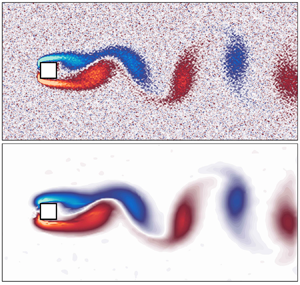
The model performance is further examined by using actual noisy PIV data. The reconstructed instantaneous vorticity field is shown in figure 9(a). The figure reveals that the model could successfully denoise the velocity fields with commendable accuracy considering the noisy input data to the model. In addition, the model shows capability of recovering the corrupted regions in the flow due to the experimental set-up. Furthermore, the relative difference of the spanwise profile of the vorticity root mean square ( $\omega _{rms}$) between the reconstructed data and the clear PIV data ( $\varepsilon (\omega _{rms})$) presented in figure 9(b) shows that the results from the model exhibit a smooth behaviour that is generally consistent with that of the clear PIV data. These results indicate that the PCDRL model can be practically applied to noisy PIV data.

Figure 9. (a) Instantaneous vorticity field of the noisy (left column) and denoised PIV data obtained from the PCDRL model (right column); (b) relative difference of the spanwise profile of the vorticity root mean square at two different streamwise locations.
4.2. POD and DMD results
In this section, the accuracy of the results from the PCDRL model is examined in terms of flow decomposition. First, the results of applying POD to the denoised data are compared with the POD results of the ground truth data. Figure 10 shows the contour plots of the leading POD modes for the vorticity field obtained from the DNS data. As can be observed from the figure, for the case of the highest noise level, i.e.  $1/SNR = 1$, all the seven true leading modes can be recovered using the denoised data, while only three modes can be recovered using the noisy data and no distinguishable features can be seen for the other modes. Furthermore, the energy plots in figure 11 represented by the normalised POD eigenvalues show that even for the case of the flow with the highest noise level, the energy contribution values of the POD modes are consistent with those obtained from the ground truth DNS data. As expected, the results from the noisy data reveal a different behaviour, especially for the cases of noise levels $1/SNR = 0.1$ and 1. Figure 12 shows a reconstructed instantaneous vorticity field of the DNS data using the first ten POD modes. As shown in the figure, the result from the PCDRL model reveals a commendable reconstruction accuracy as compared with the ground truth DNS results, whereas the result obtained from the noisy data indicates the limitation of POD in recovering the flow with the right physics.

Figure 10. Leading POD modes obtained from the DNS data. Results from the ground truth DNS (left column), PCDRL (middle column) and noisy data with  $1/SNR = 1$ (right column).

Figure 11. Normalised energy (left column) and cumulative energy (right column) of the POD modes obtained from the DNS data: (a) noisy data, where Cases 1, 2 and 3 represent the noisy DNS data at noise levels  $1/{SNR} = 0.01$, 0.1 and 1, respectively; (b) results from the PCDRL model.

Figure 12. Reconstructed instantaneous vorticity field obtained from the DNS data using the first ten POD modes. Cases 1, 2 and 3 represent the results of using noisy DNS data at noise levels  $1/{SNR} = 0.01$, 0.1 and 1, respectively.
Similar results can be obtained by applying the POD to the PIV data. As can be observed from figure 13, the seven leading POD modes obtained from the denoised PIV data are relatively consistent with the modes obtained from the clear PIV data, considering that the clean PIV data are obtained using a different experimental set-up, whereas the noisy PIV data fail to recover the modes after the third mode. Notably, the shadow region is clearly visible in some of the modes obtained from the clear PIV data, whereas no such region can be seen in the modes obtained from the denoised data. This is consistent with results from figure 9(a). The results from figure 14 further indicate the ability of the model to reconstruct the flow data with POD modes that generally have a behaviour similar to that of the clear PIV data. Furthermore, as shown in figure 15, the reconstructed instantaneous vorticity field using the first ten modes of the denoised data shows a realistic flow behaviour that is expected from the case of flow around a cylinder.

Figure 13. Leading POD modes obtained from the PIV data. Results from clear PIV (left column), PCDRL (middle column) and noisy PIV data (right column).

Figure 14. (a) Normalised energy and (b) cumulative energy of the POD modes obtained from the PIV data.

Figure 15. Reconstructed instantaneous vorticity field obtained from the results of the (a) PCDRL model and (b) noisy PIV data using the first ten POD modes.
To further investigate the dynamics of the denoised flow data, DMD is then applied to the flow data. As shown in figure 16, even in the case of the DNS data corrupted with the level of noise  $1/SNR = 1$, the DMD eigenvalues of the vorticity field show a behaviour close to that of the ground truth DNS data, whereas for the noisy data the eigenvalues scatter inside the unit circle plot, indicating a non-realistic behaviour of the system.

Figure 16. (a) DMD eigenvalues of the noisy DNS data at noise level  $1/SNR = 1$ and (b) the results from the PCDRL model visualised on the unit circle.
As for the denoised PIV data, figure 17 reveals that the eigenvalues also show good agreement with those from the clear PIV data. Notably, the leading DMD eigenvalues of the clear PIV data are not exactly located on the circumference of the unit circle as in the case of DNS data. This behaviour can be attributed to the fact that DMD is known to be sensitive to noise (Bagheri Reference Bagheri2014; Dawson et al. Reference Dawson, Hemati, Williams and Rowley2016; Hemati et al. Reference Hemati, Rowley, Deem and Cattafesta2017; Scherl et al. Reference Scherl, Strom, Shang, Williams, Polagye and Brunton2020) and, unlike the DNS data, the clear PIV contains a relatively low level of noise, which can affect the flow decomposition.

Figure 17. (a) DMD eigenvalues of the noisy PIV data and (b) the results from the PCDRL model visualised on the unit circle.
5. Conclusions
This study has proposed a DRL-based method to reconstruct flow fields from noisy data. The PixelRL method is used to build the proposed PCDRL model, wherein an agent that applies actions represented by basic filters according to a local policy is assigned to each point in the flow. Hence, the proposed model is a multi-agent model. The physical constraints represented by the momentum equation, the pressure Poisson equation and the boundary conditions are used to build the reward function. Hence, the PCDRL model is label-training data-free; that is, target data are not required for the model training. Furthermore, visualisation and interpretation of the model performance can be easily achieved owing to the model set-up.
The model performance was first investigated using DNS-based noisy data with three different noise levels. The instantaneous results and the flow statistics revealed a commendable reconstruction accuracy of the model. Furthermore, the spectral content of the flow was favourably recovered by the model, with reduced accuracy as the noise level increased. Additionally, the reconstruction error had relatively low values, indicating the general reconstruction accuracy of the model.
Real noisy and clear PIV data were used to examine the model performance. Herein, the model demonstrated its capability to recover the flow fields with the appropriate behaviour.
Furthermore, the accuracy of the denoised flow data from both DNS and PIV was investigated in terms of flow decomposition by means of POD and DMD. Most of the leading POD modes that describe the main features (coherent structures) of the flow were successfully recovered with commendable accuracy and outperformed the results of directly applying POD to the noisy data. Additionally, the DMD eigenvalues obtained from the denoised flow data exhibited behaviour similar to that of true DMD modes. These results further indicate the model's ability to recover the flow data with most of the flow physics.
This study demonstrates that the combination of DRL, the physics of the flow, which is represented by the governing equations, and prior knowledge of the flow boundary conditions can be effectively used to recover high-fidelity flow fields from noisy data. This approach can be further extended to the reconstruction of three-dimensional turbulent flow fields, for which more sophisticated DRL models with more complex spatial filters are needed. Applying such models to flow reconstruction problems can result in considerable reduction in the experimental and computational costs.
Funding
This work was supported by the ‘Human Resources Program in Energy Technology’ of the Korea Institute of Energy Technology Evaluation and Planning (KETEP), granted financial resources from the Ministry of Trade, Industry & Energy, Republic of Korea (no. 20214000000140). In addition, this work was supported by a National Research Foundation of Korea (NRF) grant funded by the Korea government (MSIP) (no. 2019R1I1A3A01058576).
Declaration of interests
The authors report no conflict of interest.
Appendix A. Open-source code
The open-source library Pytorch 1.4.0 (Paszke et al. Reference Paszke2019) was used for the implementation of the PCDRL model. The source code of the model is available at click here.
Appendix B. Asynchronous advantage actor–critic (A3C)
The asynchronous advantage actor–critic (A3C) (Mnih et al. Reference Mnih, Badia, Mirza, Graves, Lillicrap, Harley, Silver and Kavukcuoglu2016) algorithm is applied in this work. A3C is a variant of the actor–critic algorithm, which combines the policy- and value-based networks to improve performance. Figure 18 shows that the actor generates an action  $a^n$ for the given state $s^n$ based on the current policy, whilst the critic provides the value function $V(s^n)$ to evaluate the effectiveness of the action.

Figure 18. Architecture of the actor–critic algorithm.
Based on understanding of the actor–critic algorithm, A3C also has two sub-networks: the policy and value networks. Herein,  $\theta _p$ and $\theta _v$ are used to represent the parameters of each network. The gradients of $\theta _p$ and $\theta _v$ can be calculated as follows:
 \begin{gather} R^n = r^n + \gamma r^{n+1} + \cdots + \gamma^{(N-1)}r^N + \gamma^{(N)}V(s^N), \end{gather}
 \begin{gather}d\theta_v = {\boldsymbol{\nabla}_\theta}_v (R^n - V(s^n))^2, \end{gather}
 \begin{gather}A(a^n,s^n) = R^n - V(s^n), \end{gather}
 \begin{gather}d\theta_p ={-} {\boldsymbol{\nabla}_\theta}_p \log {\rm \pi}(a^n,s^n) A(a^n,s^n), \end{gather}
where  $A(a^n,s^n)$ is the advantage.
Appendix C. PixelRL
A3C is modified in this study to a fully convolutional form (Furuta et al. Reference Furuta, Inoue and Yamasaki2020), and its architecture can be found in figure 19. Through this approach, all the agents share the same parameters, which saves on computational cost and trains the model more efficiently compared with the case where agents need to train their models individually. The size of the receptive field can also affect the performance of the CNN network, and a large receptive field can result in superior capture connections between points. Therefore, a receptive field ( $3\times 3$) is used in the architecture; that is, the outputs of the policy and value networks at a specific pixel will be affected by the pixel and its surrounding neighbour pixels. Figure 19 shows that the input flow field data first pass through four convolutional and leaky rectified linear unit (ReLU) (Goodfellow, Bengio & Courville Reference Goodfellow, Bengio and Courville2016) layers and are then inputted to the policy and value networks, respectively. The policy network comprises three convolutional layers with a ReLU activation function, a ConvGRU layer and a convolutional layer with a SoftMax activation function (Goodfellow et al. Reference Goodfellow, Bengio and Courville2016), and its output is the policy. The first three layers of the value network are the same as the first three layers of the policy network, and the value function is finally obtained through the convolutional layer with a linear function.

Figure 19. Architecture of the fully convolutional A3C.
The gradients of the parameters  $\theta _p$ and $\theta _v$ are then defined on the basis of the architecture of the fully convolutional A3C:
 \begin{gather} {\boldsymbol{R}}^n = {\boldsymbol{r}}^n + \gamma {\boldsymbol{W}} \ast {\boldsymbol{r}}^{n+1} + \cdots + \gamma^{(N-1)} {\boldsymbol{W}}^{(N-1)} \ast {\boldsymbol{r}}^N + \gamma^{(N)} {\boldsymbol{W}}^{(N)} \ast {\boldsymbol{V}}({\boldsymbol{s}}^N), \end{gather}
 \begin{gather}d\theta_v = {\boldsymbol{\nabla}}_{\theta_v} \frac{1}{I\times J} \textbf{1}^\top \{ ({\boldsymbol{R}}^n - {\boldsymbol{V}}({\boldsymbol{s}}^n)) \odot ({\boldsymbol{R}}^n - {\boldsymbol{V}}({\boldsymbol{s}}^n))\} \textbf{1}, \end{gather}
 \begin{gather}{\boldsymbol{A}}({\boldsymbol{a}}^n,{\boldsymbol{s}}^n) = {\boldsymbol{R}}^n - {\boldsymbol{V}}({\boldsymbol{s}}^n), \end{gather}
 \begin{gather}d\theta_p ={-} {\boldsymbol{\nabla}}_{\theta_p} \frac{1}{I\times J} \textbf{1}^\top \{ \log \boldsymbol{\rm \pi} ({\boldsymbol{a}}^n,{\boldsymbol{s}}^n) \odot {\boldsymbol{A}}({\boldsymbol{a}}^n,{\boldsymbol{s}}^n) \} \textbf{1}, \end{gather}
where  ${\boldsymbol {R}}^n$, ${\boldsymbol {r}}^n$, ${\boldsymbol {V}}({\boldsymbol {s}}^n)$, ${\boldsymbol {A}}({\boldsymbol {a}}^n,{\boldsymbol {s}}^n)$ and $\boldsymbol {{\rm \pi} } ({\boldsymbol {a}}^n,{\boldsymbol {s}}^n)$ are the matrices whose $(i, j)$th elements are $R^n_{i,j}$, $r^n_{i,j}$, $V(s^n_{i,j})$, $A(a^n_{i,j},s^n_{i,j})$ and ${\rm \pi} (a^n_{i,j},s^n_{i,j})$, respectively. Here, $\ast$ is the convolution operator, $\textbf {1}$ is the all-ones vector and $\odot$ is element-wise multiplication. Additionally, ${\boldsymbol {W}}$ is a convolution filter weight, which is updated simultaneously with $\theta _p$ and $\theta _v$ such that
 \begin{align} d{\boldsymbol{W}} &={-} {\boldsymbol{\nabla}}_{{\boldsymbol{W}}} \frac{1}{I\times J} \textbf{1}^\top \{ \log \boldsymbol{\rm \pi} ({\boldsymbol{a}}^n,{\boldsymbol{s}}^n) \odot {\boldsymbol{A}}({\boldsymbol{a}}^n,{\boldsymbol{s}}^n) \} \textbf{1} \nonumber\\ & \quad + {\boldsymbol{\nabla}}_{{\boldsymbol{W}}} \frac{1}{I\times J} \textbf{1}^\top \{ ({\boldsymbol{R}}^n - {\boldsymbol{V}}({\boldsymbol{s}}^n)) \odot ({\boldsymbol{R}}^n - {\boldsymbol{V}}({\boldsymbol{s}}^n))\} \textbf{1}. \end{align}
Notably, after the agents complete their interaction with the environment, the gradients are acquired simultaneously, which means that the number of asynchronous threads is one; that is, A3C is equivalent to advantage actor–critic (A2C) in the current study (Clemente, Castejón & Chandra Reference Clemente, Castejón and Chandra2017).
Appendix D. Denoising action set
The action set for removing the noise of the flow fields is shown in table 1. The agent can take the following nine possible actions: do nothing, apply six classical image filters or plus/minus a  $\textit {Scalar}$. The actions in this study are discrete and determined empirically. The table shows that the parameters $\sigma _c$, $\sigma _s$ and $\sigma$ represent the filter standard deviation in the colour space, the coordinate space and the Gaussian kernel, respectively. The $\textit {Scalar}$ in the $8$th and $9$th actions is determined on the basis of the difference between the variance of the clear and noisy data.
Table 1. Action set for the denoising process.


 Open access